Dual Image Deblurring Using Deep Image Prior

Abstract

Blind image deblurring, one of the main problems in image restoration, is a challenging, ill-posed problem. Hence, it is important to design a prior to solve it. Recently, deep image prior (DIP) has shown that convolutional neural networks (CNNs) can be a powerful prior for a single natural image. Previous DIP-based deblurring methods exploited CNNs as a prior when solving the blind deburring problem and performed remarkably well. However, these methods do not completely utilize the given multiple blurry images, and have limitations of performance for severely blurred images. This is because their architectures are strictly designed to utilize a single image. In this paper, we propose a method called DualDeblur, which uses dual blurry images to generate a single sharp image. DualDeblur jointly utilizes the complementary information of multiple blurry images to capture image statistics for a single sharp image. Additionally, we propose an adaptive $L_2\_$SSIM loss that enhances both pixel accuracy and structural properties. Extensive experiments show the superior performance of our method to previous methods in both qualitative and quantitative evaluations.

1. Introduction

Motion blur is a common artifact caused by the relative motion between the camera and the scene during exposure. In practice, when we obtain images from cameras equipped in the mobile embedded systems, the images are often blurred because they are usually captured with hand-held cameras. The unwanted blur artifacts not only degrade the image quality but also result in the loss of important information in the image. Consequently, blurry images deteriorate the performance of various computer vision tasks, such as image classification [1,2,3], object detection [4,5,6], and segmentation [7,8,9]. Accordingly, numerous image deblurring studies have been actively proposed to remove blur artifacts and restore sharp images.

Given a blurry image y, the blur process is typically modeled as a convolution operation of a latent sharp image x and a blur kernel k as follows:

$$y=k\otimes x+n,$$

(1)

where ⊗ denotes the convolution operator and n is the noise. The goal of blind image deblurring is to estimate the sharp image and the blur kernel simultaneously when the blur kernel is unknown. This is a classical ill-posed problem because x and k can have multiple solutions. Owing to the ill-posed nature of the problem, conventional deblurring studies constrain the solution space by leveraging various priors and regularizers.

Recently, extensive studies [10,11,12,13,14] based on deep learning (DL) have been performed on image deblurring. Most of them employ deep convolutional neural networks (CNNs) and trained them on a large-scale dataset of blurry/sharp image pairs [15]. CNNs implicitly learn more general priors by capturing the natural image statistics from a large number of blurry/sharp image pairs. DL-based methods have provided superior results. However, collecting such a large dataset is difficult and expensive [16]. In contrast to DL-based data-driven approaches, Ulyanov et al. [17] proposed a deep image prior (DIP), which is based on self-supervised learning, and showed that a CNN can capture the low-level statistics of a single natural image. Their method performed remarkably well in low-level vision tasks, such as denoising, super-resolution, and inpainting. Inspired by this, Ren et al. [18] suggested the SelfDeblur framework to solve the single image blind deblurring problem. Given a single blurry image, the SelfDeblur estimates the latent sharp image and the blur kernel simultaneously by jointly optimizing the image generator network and kernel estimator network. However, the SelfDeblur cannot perform deblurring in the case of multiple blurry images. This is because the architecture of the SelfDeblur is strictly designed to leverage only the internal statistics of a single blurry image. Although using multiple observations for image deblurring is beneficial [19,20], most of self-supervised learning approaches do not completely leverage the internal information of given multiple images.

We propose a method called DualDeblur that aims to restore a single sharp image from two given blurry observations. In many practical scenarios, we can capture multiple images of the same physical scene. At this time, we obtain multiple blurry images under various conditions through multiple captures. For example, let us consider two blurry images shown in Figure 1b,c. They share the same latent sharp image as shown in Figure 1a. Thus, the sharp images restored from Figure 1b,c should be the same. Hence, we can further constrain the solution space. Specifically, our DualDeblur comprises a single image generator and two blur kernel estimators. The image generator aims to estimate a sharp image, which is latent in two blurry images. Each blur kernel estimator estimates the blur kernel for each blurry image. Thereafter, we jointly optimize the image generator and blur kernel estimators by comparing the reblurred images and given blurry images. Here, the reblurred images are generated by the blur process of the predicted image and the estimated blur kernels. Through this joint optimization process, our image generator learns a strong prior for a single sharp image by using the complementary information of multiple images.

In addition, we propose an adaptive $L_2\_$SSIM loss to enhance both pixel-wise accuracy and structure details. Most DIP-based methods use the $L_2$ loss to minimize the difference in pixel values between the target image and restored image. In our task, simply using the $L_2$ loss may deteriorate the restoration performance because the target image is blurry. Thus, the $L_2$ loss is insufficient to restore the detailed textures. Hence, many restoration methods involve replacing the $L_2$ loss with structural properties loss, such as the SSIM loss [9], MS-SSIM loss [22], and FSIM loss [23]. However, using only the SSIM loss has several limitations. SSIM does not consider pixel-wise accuracy. Therefore, comparing corrupted structures may lead to unexpected resulting images. To tackle this, our adaptive $L_2\_$SSIM loss adjusts the weight for each training step through a weighted sum that considers the characteristics of $L_2$ and SSIM. At the beginning of training, most of the weight is focused on $L_2$, which is decreased exponentially, according to the iterations. Hence, pixel-wise accuracy is ensured by focusing on $L_2$ in the early stages of training. Increasing the pixel-wise accuracy at an early stage of training can prevent unexpected structures in the resulting images. In the remaining stages of training, we exponentially increase the weight of the SSIM loss to preserve the structural properties. Through this process, our reconstruction loss ensures both pixel-wise accuracy and structural properties.

Figure 1 shows the effectiveness of our method. Generally, large blurs often occur when the images are taken from cameras with fast movement in the night environments (see Figure 1b,c). In this case, previous classical methods often fail to restore the sharp images, as shown in Figure 1d,e. This is because the priors utilized in the methods are subjective and cannot accurately capture the intrinsic distribution of natural images and blur kernels [24]. As shown in Figure 1f,g, SelfDeblur [18] also fails to estimate the kernel for severely blurred images and does not appropriately deblur images. However, the proposed DualDeblur successfully estimates two blur kernels using two severely blurred images and generates a superior resulting image with many textures. Our experiments show that DualDeblur performs better than other comparative methods, both quantitatively and qualitatively.

The following are the main contributions of this study:

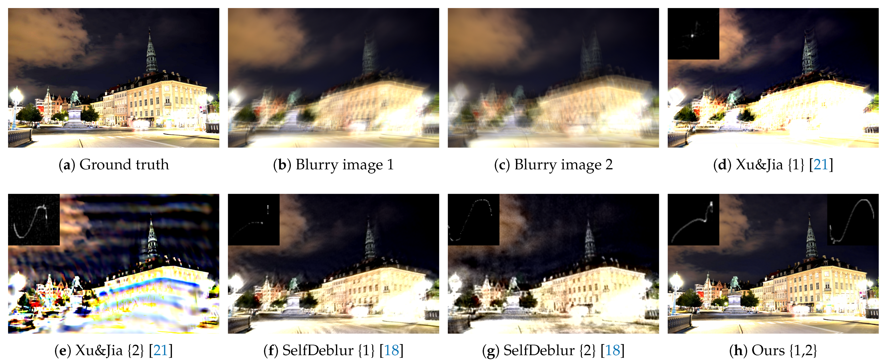
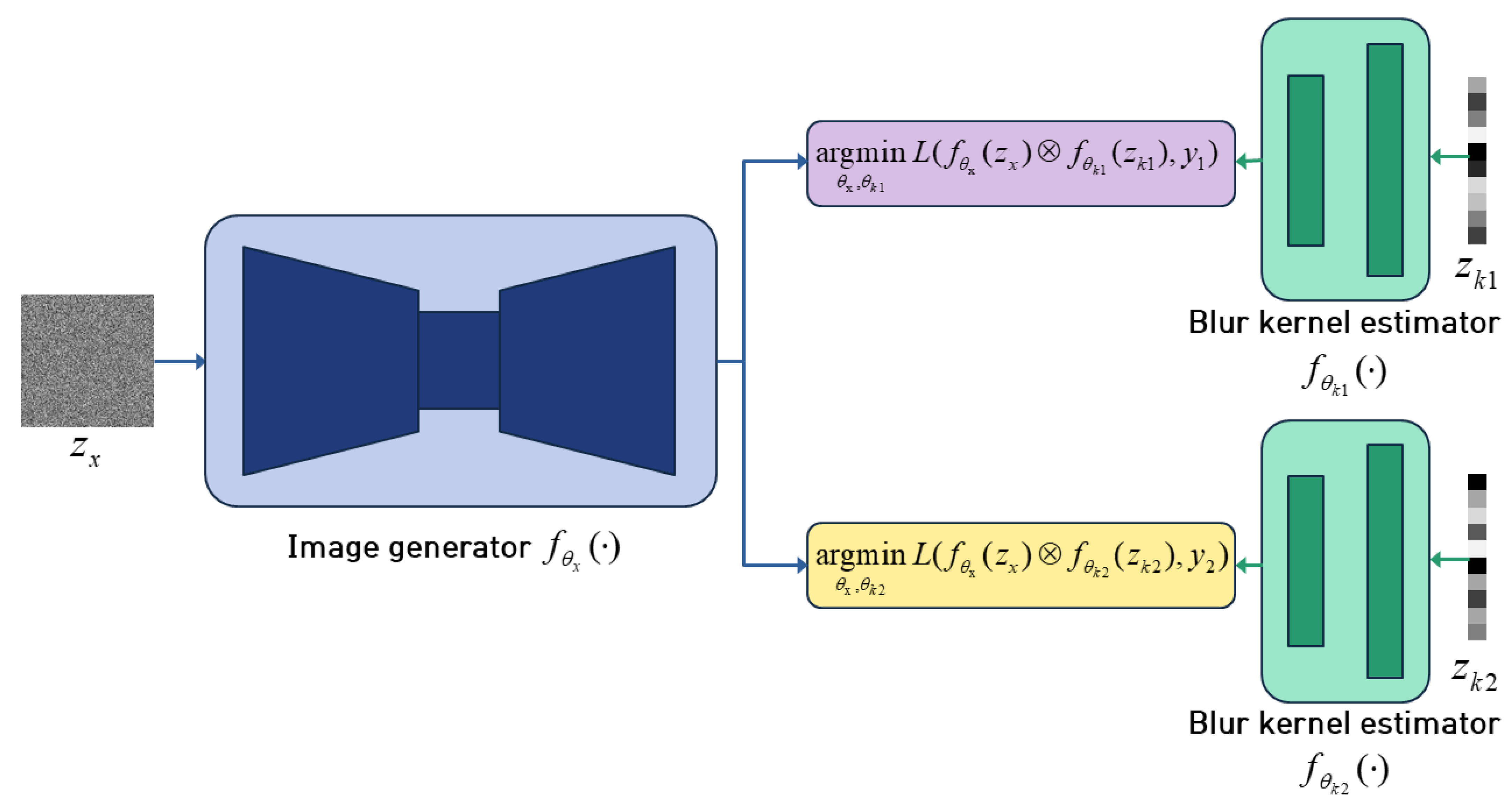
• We propose a DIP-based deblurring method called DualDeblur using two blurry images of the same scene. Multiple images are used to jointly optimize complementary information.
• We propose an adaptive $L_2\_$SSIM loss that adjusts the weights of both $L_2$ and SSIM for each optimization step. From this, we ensure both pixel-wise accuracy and structural properties in the deblurred image.
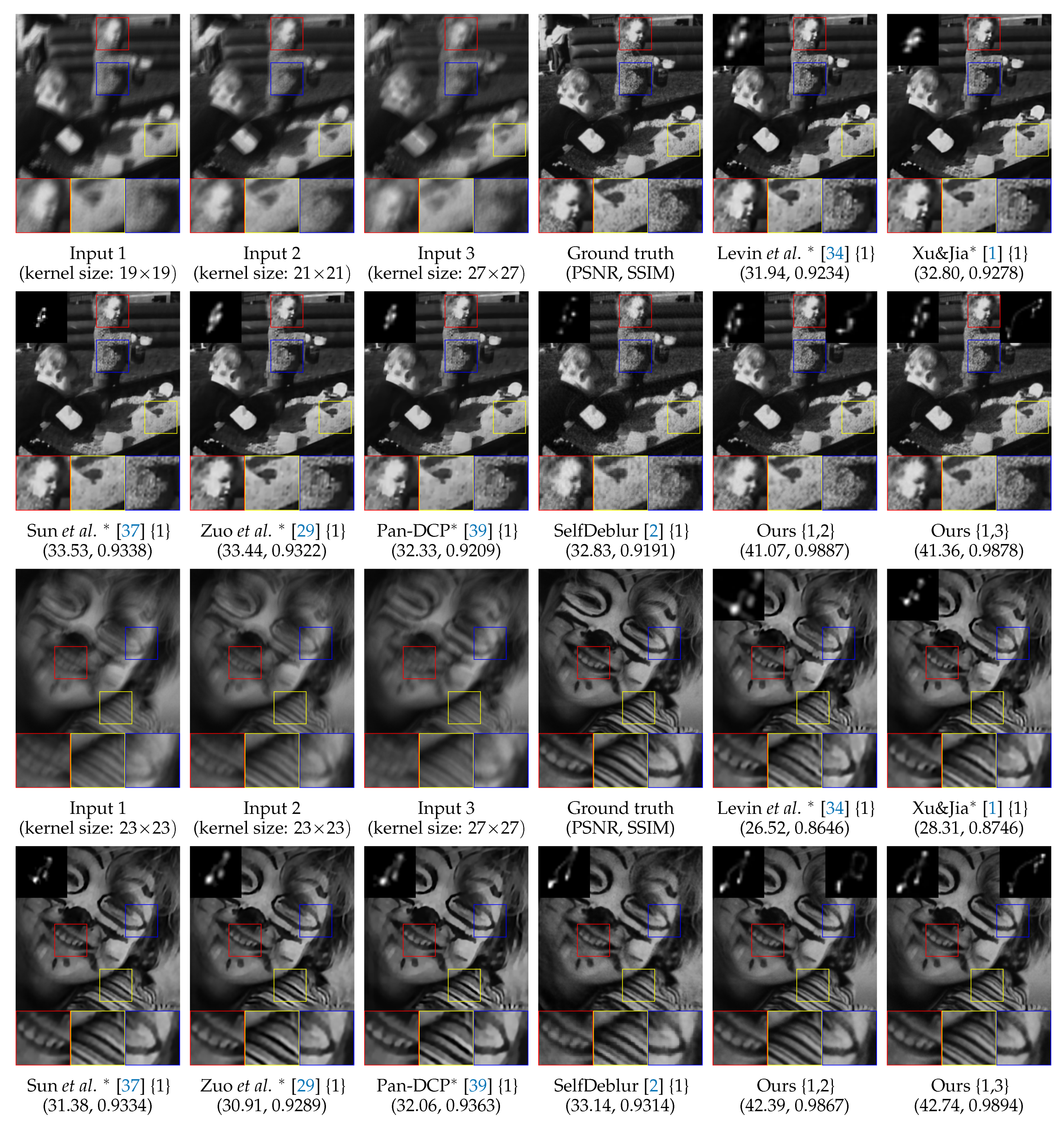
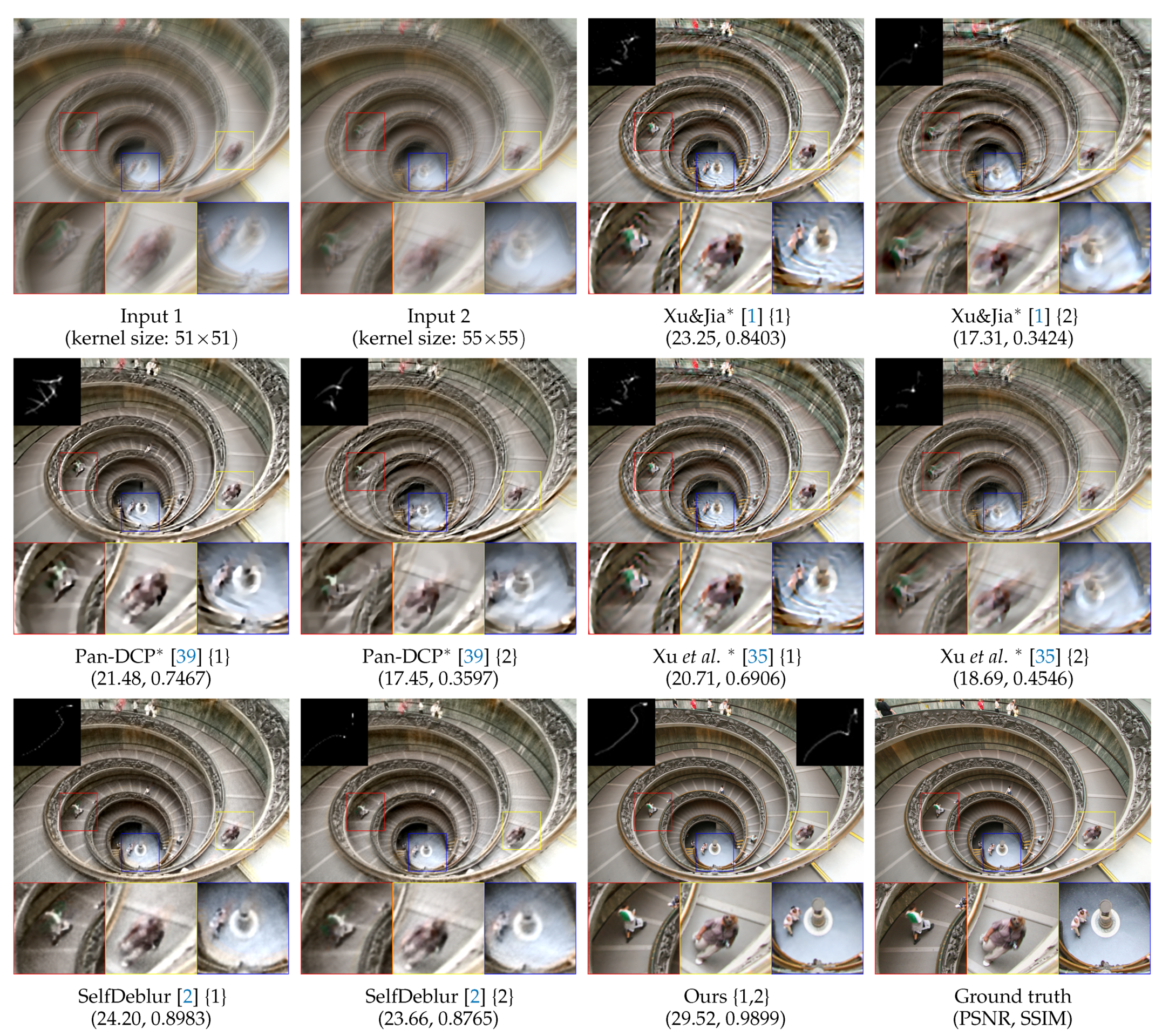
• The experimental results show that our method is quantitatively and qualitatively superior to previous methods.

2. Related Works

In this section, we briefly introduce the existing image deblurring methods based on optimization and DL [25].

2.1. Optimization-Based Image Deblurring

Image deblurring, one of the classical inverse problems, aims to restore a sharp latent image from a given blurry image. Owing to the ill-posed nature of the deblurring problem, most traditional methods have been proposed to constrain the solution space by using various priors or regularizers, such as TV regularizations [26,27], gradient priors [21], sparsity priors [28], gradient sparsity priors [29], Gaussian scale mixture priors [30], hyper-Laplacian priors [31], ${\ell }_1$/${\ell }_2$-norms [32], variational Bayes approximations [33,34], ${\ell }_0$-norms [35,36], patch-based statistical priors [37,38], adaptive sparse priors [19], and dark channel priors [39]. By taking advantage of those priors, the traditional methods jointly estimated the sharp image and blur kernel from the blurry image. However, most of these methods heavily rely on the accurate selection of regularizers or priors. Furthermore, when the blur kernel is large and complex, their methods often fail to restore the sharp image.

2.2. DL-Based Image Deblurring

Recently, DL [25]-based methods were widely developed to solve the image deblurring problem. Early DL-based deblurring methods [40,41] focused only on estimating blur kernels using DL. Sun et al. [40] proposed to predict the probabilistic distribution of motion blur at the patch level, using a CNN. Chakrabarti et al. [41] presented a CNN to predict the complex Fourier coefficients of a deconvolution filter to be applied to the input patch for restoration. Unlike traditional approaches of using CNNs as a kernel estimation process, Nah et al. [10] proposed to directly predict the deblurred output without an additional kernel estimation process by using multi-scale CNNs. Motivated by the multi-scale approach, Tao et al. [12] proposed to reduce the memory size using a long short-term memory (LSTM)-based scale-recurrent network. Zhang et al. [14] proposed a multi-level CNN that uses a multi-patch hierarchy as input to exploit a multi-patch localized-to-coarse approach. Ulyanov et al. [17] suggested DIP, showing that CNNs can work satisfactorily as priors for a single image. However, there is a limitation to capturing the characteristics of the blur kernel, because the DIP network consists of CNNs that contain only image statistics [18]. To tackle this, Ren et al. [18] suggested the SelfDeblur to solve the blind deblurring problem. SelfDeblur [18] adopted a CNN to capture image statistics. To overcome the aforementioned drawback of DIP, they employed a fully connected network (FCN) to model the prior of the blur kernel. Although SelfDeblur [18] effectively solves the blind deblurring problem, its structure can only handle a single image and cannot appropriately utilize multiple images. In contrast to SelfDelbur, our DualDeblur is designed with a structure that can utilize multiple images that share a single sharp image.

3. Proposed Method

In this section, we describe the blur process for two blurry images and the proposed DualDeblur framework, using two blurry images. Additionally, we introduce an adaptive $L_2\_$SSIM loss that considers both pixel-wise accuracy and perceptual properties. Subsequently, we summarize the optimization process of the proposed method.

3.1. DualDeblur

Given two blurry observations $y_1$ and $y_2$, the blur process can be formulated as follows:

$$y_1=k_1\otimes x+n_1,y_2=k_2\otimes x+n_2,$$

(2)

where x denotes a latent sharp image, and $k_1$ and $k_2$ represent two blur kernels corresponding to each blurry observation, respectively. Our DualDeblur predicts a single sharp image x using two blurry images, $y_1$ and $y_2$. As depicted in Figure 2, DualDeblur consists of an image generator $f_{{\theta }_x}(·)$ and blur kernel estimators $f_{{\theta }_{k1}}(·)$ and $f_{{\theta }_{k2}}(·)$.

Table 1. Architecture $f_{{\theta }_x}$. We adopt Unet [7] with a skip connection as the architecture of $f_{{\theta }_x}$. Conv2d represents a 2D convolution operation, “lReLU” denotes a leaky ReLU, and ⊕ denotes the channel-wise concatenation. Kernel ($m,n\times n,p$) represents the number of filters m, filter sizes $n\times n$, and padding p. We implement downsampling with stride 2 and upsampling with bilinear interpolation. C represents image channels, and $W_x\times H_x$ the image size.

Input: ${\mathit{z}}_{\mathit{x}}$($8\times {\mathit{W}}_{\mathit{x}}\times {\mathit{H}}_{\mathit{x}})$ of a uniform distribution
Output: latent image $\widehat{x}(C\times W_x\times H_x)$
Encoder	Operation	Kernel	In→Out	Decoder	Operation	Kernel	In→Out
Encoder 1	Conv2d, lReLU	128, 3 × 3, 1	$z_x\to e_1$	Decoder 1	Conv2d, lReLU	128, 3 × 3, 1	$e_5\oplus s_5\to d_1$
	Conv2d, lReLU	16, 3 × 3, 1	$e_1\to s_1$
Encoder 2	Conv2d, lReLU	128, 3 × 3, 1	$e_1\to e_2$	Decoder 2	Conv2d, lReLU	128, 3 × 3, 1	$d_1\oplus s_4\to d_2$
Skip 2	Conv2d, lReLU	16, 3 × 3, 1	$e_2\to s_2$
Encoder 3	Conv2d, lReLU	128, 3 × 3, 1	$e_2\to e_3$	Decoder 3	Conv2d, lReLU	128, 3 × 3, 1	$d_2\oplus s_3\to d_3$
Skip 3	Conv2d, lReLU	16, 3 × 3, 1	$e_3\to s_3$
Encoder 4	Conv2d, lReLU	128, 3 × 3, 1	$e_3\to e_4$	Decoder 4	Conv2d, lReLU	128, 3 × 3, 1	$d_3\oplus s_2\to d_4$
Skip 4	Conv2d, lReLU	16, 3 × 3, 1	$e_4\to s_4$
Encoder 5	Conv2d, lReLU	128, 3 × 3, 1	$e_4\to e_5$	Decoder 5	Conv2d, lReLU	128, 3 × 3, 1	$d_4\oplus s_1\to d_5$
Skip 5	Conv2d, lReLU	16, 3 × 3, 1	$e_5\to s_5$
Output layer	Conv2d, $Sigmoid$	C, 1 × 1, 0	$d_5\to \widehat{x}$

presents the detailed architecture of our image generator $f_{{\theta }_x}(·)$. The image generator $f_{{\theta }_x}(·)$ is learned as a network $\widehat{x}=f_{{\theta }_x}\left(z_x\right)$ mapping the uniform distribution $z_x$ to an image $\widehat{x}$.

Table 2. The architecture $f_{{\theta }_{ki}}(·)$. We adopt a FCN as each blur kernel estimator network $f_{{\theta }_{ki}}(·)$. $W_{ki}\times H_{ki}$ represents blur kernel sizes. $f_{{\theta }_{ki}}(·)$ takes a 200-dimensional input and has 1000 nodes in the hidden layer and $W_{ki}\times H_{ki}$ nodes in the last layer. The 1D output is reshaped to a 2D blur kernel size.

Input: ${\mathit{z}}_{\mathit{k}\mathit{i}}$(200) of uniform distributions, blur kernel size of ${\mathit{W}}_{\mathit{k}\mathit{i}}\times {\mathit{H}}_{\mathit{k}\mathit{i}}$
Output: blur kernel $k_i(W_{ki}\times H_{ki})$
FCN	Operation
Layer 1	Linear (200, 1000), $ReLU$
Layer 2	Linear (1000, $W_{ki}\times H_{ki}$), $SoftMax$

shows our kernel estimators $f_{{\theta }_{k1}}(·)$ and $f_{{\theta }_{k2}}(·)$. The blur kernel estimator $f_{{\theta }_{k1}}(·)$ is learned as a network ${\widehat{k}}_1=f_{{\theta }_{k1}}\left(z_{k1}\right)$ mapping the uniform distribution 1-D vector $z_{k1}$ to a 2-D reshaped blur kernel ${\widehat{k}}_1$. Similarly, the blur kernel estimator $f_{{\theta }_{k2}}(·)$ is learned as a network ${\widehat{k}}_2=f_{{\theta }_{k2}}\left(z_{k2}\right)$ mapping the uniform distribution 1-D vector $z_{k2}$ to a 2-D reshaped blur kernel ${\widehat{k}}_2$. Networks $f_{{\theta }_{k1}}(·)$ and $f_{{\theta }_{k2}}(·)$ are dual architectures designed for two blurry images. ${\widehat{k}}_1$ and ${\widehat{k}}_2$ are the estimated blur kernels corresponding to $y_1$ and $y_2$, respectively. DualDeblur jointly optimizes $f_{{\theta }_x}(·)$, $f_{{\theta }_{k1}}(·)$, and $f_{{\theta }_{k2}}(·)$ by comparing $y_1$ and ${\widehat{x}}_1\otimes {\widehat{k}}_1$, as well as $y_2$ and ${\widehat{x}}_2\otimes {\widehat{k}}_2$ through the proposed loss function, as explained in the following.

3.2. Adaptive $L_2\_$SSIM Loss

In this sub-section, we propose an adaptive $L_2\_$SSIM loss to enhance both pixel-wise accuracy and perceptual properties. We adjust the weights of each training step with a weighted sum that considers the properties of $L_2$ and SSIM. First, we introduce the $L_2$ and SSIM losses.

When solving the restoration problem, the $L_2$ loss is usually used and is formulated as follows:

$$L_2=\sum _{i=1}^2{∥{\widehat{k}}_i\otimes \widehat{x}-y_i∥}^2,$$

(3)

where i denotes the i-th observation, and $L_2$ increases the pixel-wise accuracy by minimizing the pixel values between the target image and the restored image. However, in the case of $L_2$, the output image tends to be blurry and lacks high-frequency textures [42,43]. In our case, using only $L_2$ is even worse because both y and $k\otimes x$ are blurry images. To overcome the limitation, the SSIM loss, which preserves perceptual features is also used. SSIM captures the luminance, contrast, and structure of an image [9]. Here, $L_{SSIM}$ is formulated as follows:

$$L_{SSIM}=\sum _{\mathrm{i}=1}^2(1-SSIM({\widehat{k}}_i\otimes \widehat{x},y_i)),$$

(4)

However, because the SSIM loss does not consider pixel-wise accuracy, collapsed structures in the blurry observations may lead to an unexpected structure in the resulting image. Therefore, we propose an adaptive $L_2\_$SSIM loss to preserve the strengths of each loss and compensate for the weaknesses of each loss. The proposed adaptive $L_2\_$SSIM loss ($L_{L_2\_SSIM}$) is formulated as follows:

$$\begin{array}{c}{L}_{L_2\_SSIM}\left(t\right)=\omega \left(t\right)\alpha L_2+(1-\omega \left(t\right))L_{SSIM},\hfill \\ \omega \left(t\right)=exp(-\frac{t}{\gamma }),\end{array}$$

(5)

where $\omega \left(t\right)$ denotes a weighting function that adjusts the weights of the $L_2$ and SSIM losses according to each tth step, and $\alpha$ represents a parameter that adjusts the scale of the $L_2$ loss. $\gamma$ denotes a parameter that adjusts the range of the steps affected by the $L_2$ loss. At the beginning of the step, the weights of the $L_2$ loss account for most of the total weights to focus on pixel-wise accuracy so that it does not result in unexpected structures. Hence, we reduce the weights of the $L_2$ loss and increase those of the $L_{SSIM}$ loss to preserve the structure content of the image. As a result, our reconstruction loss not only increases the pixel-wise accuracy, but also preserves the structural details of the image. The effectiveness of the proposed reconstruction loss was demonstrated in an ablation study in Section 4.5.

The final optimization process of DualDeblur is summarized in Algorithm 1. Here, T denotes the total training iteration, and ${\theta }_{k1}$, ${\theta }_{k2}$ and ${\theta }_x$ represent network parameters corresponding to $f_{{\theta }_{k1}}(·)$, $f_{{\theta }_{k2}}(·)$ and $f_{{\theta }_x}(·)$, respectively. DualDeblur estimates a restored image and two blur kernels. Thereafter, it generates two reblurred images using a convolution operation and compares them with $y_1$ and $y_2$, respectively, through the $L_{L_2\_SSIM}$ loss in Equation (5). By optimizing all the networks simultaneously, the image generator $f_{{\theta }_x}(·)$ jointly utilizes the complementary information of the two blurry images. Finally, we obtain the restored image and blur kernels from T iterations.

Algorithm 1 DualDeblur optimization process

Input: blurry images $y_1,y_2$ and T iterations Output: restored image $\widehat{x}$, estimated blur kernels ${\widehat{k}}_1$ and ${\widehat{k}}_2$  1: Sample $z_x$, $z_{k1}$, and $z_{k2}$ from uniform distribution  2: for $t=1$ to T do  3:     perturb $z_x$  4:     $\widehat{x}=f_{{\theta }_x}^{t-1}\left(z_x\right)$  5:    ${\widehat{k}}_1=f_{{\theta }_{k1}}^{t-1}\left(z_{k1}\right)$  6:     ${\widehat{k}}_2=f_{{\theta }_{k2}}^{t-1}\left(z_{k2}\right)$  7:     Compute the gradients of ${\theta }_x^{t-1},{\theta }_{k1}^{t-1}$ and ${\theta }_{k2}^{t-1}$ w.r.t. $L_{L_2\_SSIM}\left(t\right)$  8:     Update ${\theta }_x^t,{\theta }_{k1}^t$ and ${\theta }_{k2}^t$ using the ADAM [44]  9: end for  10: $\widehat{x}=f_{{\theta }_x}^T\left(z_x\right),$${\widehat{k}}_1=f_{{\theta }_{k1}}^T\left(z_{k1}\right)$ and ${\widehat{k}}_2=f_{{\theta }_{k2}}^T\left(z_{k2}\right)$

4. Experimental Results

4.1. Dataset

To evaluate the performance of our method, we used two image deblurring benchmark datasets: the Levin test set [33] and the Lai test set [45]. The proposed method solves the deblurring problem by using two observations. In this case, there are two possible scenarios. First, two observations are degraded by a similar degree of blur artifacts (soft pairs). Second, the degrees of blur artifacts are very different from each other (hard pairs). To simulate these cases, we divided each test set into soft and hard pairs and used them for evaluation. The two test sets are discussed in the following.

1

Levin test set [33]: In their seminal work, Levin et al. [33] provided 8 blur kernels with size of $k\times k$, where $k=13,15,17,19,21,23,27$ and 4 sharp images, resulting in 32 blurry gray-scale images with size of $255\times 255$. To evaluate our method, we divided the soft and hard pairs on the basis of difference in blur kernel size. If the difference was less than 5 pixels, we classified such an image pair as a soft pair, and vice versa as a hard pair. Following this pipeline, we randomly selected 7 soft pairs and 7 hard pairs, totaling to 14 blurry pairs per image. In short, we prepared a total of 56 pairs of blurry images for evaluation. The composition of the Levin test set [33] is described in detail in

Table 3. Configurations of Levin test set [33] and Lai test set [45].

Test Set	# GT Images	# Blur Kernel	# Blur Images	# Soft Pair	# Hard Pair	# Total Pair
Levin test set [33]	4	8	32	28	28	56
Lai test set [45]	25	4	100	25	100	125

. Specifically, the soft pairs comprised $[13,15], [15,17], [17,19], [19,21], [21,23a], [21,23a]$, and $[23a,23b]$. Here, each number represents the blur kernel size of k. For example, [11, 13] means that the blur kernel sizes 13 × 13 and 15 × 15 are paired. Because the Levin test set contains two blur kernels with a size of 23 × 23, we denote each as $23a$ and $23b$. The hard pairs contained $[13,27], [15,27], [17,27], [19,27], [21,27], [23a,27]$, and $[23b,27]$.

2

Lai test set [45]: We further compared our method using the Lai test set [45], which contains RGB images of various sizes. The Lai test set comprises 4 blur kernels and 25 sharp images, resulting in 100 blurry images. It is divided into five categories: $Manmade,Natural,People,Saturated,$ and $Text$, with 20 images for each category. The sizes of the 4 blur kernels are $31\times 31, 51\times 51, 55\times 55,$ and $75\times 75$. Thus, we prepared a soft pair (i.e., $[51,55]$), and 4 hard pairs (i.e., $[31,51], [31,75], [51,75]$, and $[55,75]$). As described in Table 3, there are 25 sharp images and 5 blur kernel pairs; a total of 125 pairs of blur images are used for evaluation.

4.2. Implementation Details

We implemented our DualDeblur using Pytorch [46]. The networks were optimized using Adam [44] with a learning rate of $1\times {10}^{-2}$, ${\beta }_1$ = 0.9, and ${\beta }_2$ = 0.999. In our experiments, the total number of iterations was 5000, and the learning rate was decayed by multiplying by 0.5 for every 2000, 3000, and 4000 iterations. We empirically set values of $\alpha$ and $\gamma$ in Equation (5) as $\alpha =10$ and $\gamma =100$. Following [17,18], we sampled the initial $z_x$, $z_{k1}$ and $z_{k2}$ from the uniform distribution with a fixed random seed 0. Notably, all the experiments of our model were conducted using a single NVIDIA TITAN-RTX GPU.

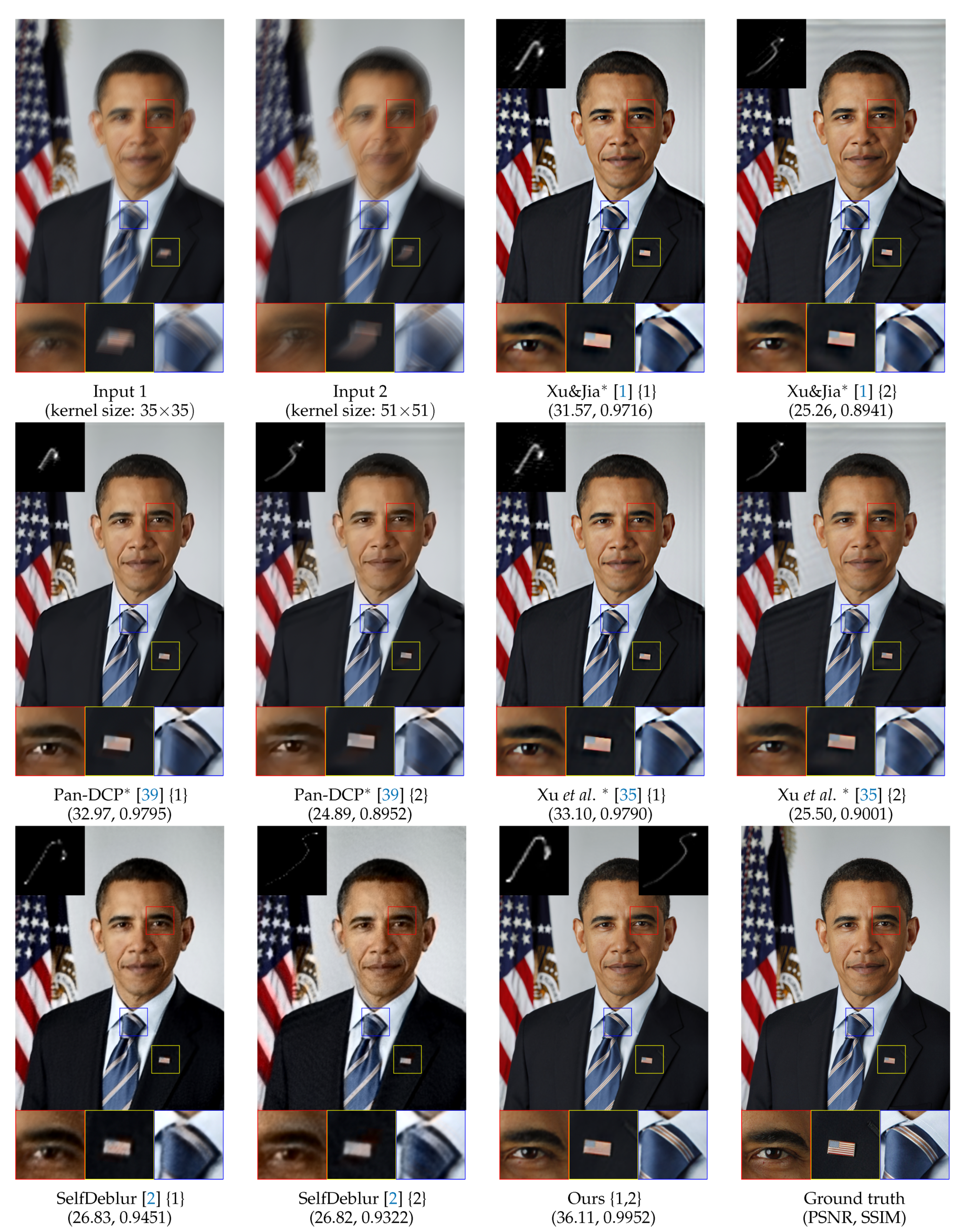
4.3. Comparison on the Levin Test Set

For the Levin test set [33], we compared our DualDeblur with the existing blind deconvolution methods (i.e., Krishnan et al. [32], Levin et al. [33], Cho&Lee [30], Xu&Jia [21], Sun et al. [37], Zuo et al. [29], and Pan-DCP [39]), and a DIP-based deblurring method (i.e., SelfDeblur [18]). Ref. [34] was used as the deconvolution to generate the final results of the previous methods. For quantitative comparison, we calculated the PSNR and SSIM [9] metrics using the codes provided by [18]. Moreover, we reported FSIM [23] and LPIPS [43] distance to evaluate the perceptual similarity. We also compared the error ratio [34], which was formulated by the sum of squared differences between deconvolution with the estimated kernels and deconvolution with the ground truth kernels.

We computed the average PSNR, SSIM, error ratio, FSIM and LPIPS on the Levin test set for various methods (see

Table 4. Quantitative comparisons on the Levin test set [33]. * indicates that the method uses the non-blind deconvolution method of [34] to produce the final result. The best results are highlighted. Results of the blur kernel “Avg.” means the averagePSNR, SSIM, error ratio, FSIM and LPIPS results for all blur kernels.

Method	Blur Kernel	PSNR ↑	SSIM ↑	Error Ratio ↓	FSIM↑	LPIPS ↓	Method	Blur Kernel	PSNR ↑	SSIM ↑	Error Ratio↓	FSIM ↑	LPIPS ↓
known k *	13	36.53	0.9659	1.0000	0.8868	0.0530	known k *	15	35.33	0.9525	1.0000	0.8167	0.0919
Krishnan et al. * [32]	13	34.88	0.9575	1.1715	0.9116	0.0604	Krishnan et al. * [32]	15	34.87	0.9481	1.0563	0.7862	0.1201
Cho & Lee * [30]	13	33.93	0.9532	1.2536	0.8578	0.0925	Cho & Lee * [30]	15	33.88	0.9429	1.3191	0.7891	0.1226
Levin et al. * [34]	13	34.29	0.9533	1.3454	0.8213	0.0922	Levin et al. * [34]	15	30.94	0.8950	2.5613	0.8003	0.1199
Xu & Jia * [21]	13	34.10	0.9532	1.2846	0.8612	0.0939	Xu & Jia * [21]	15	33.04	0.9355	1.4272	0.7763	0.1417
Sun et al. * [37]	13	36.24	0.9659	0.9933	0.8639	0.0685	Sun et al. * [37]	15	34.96	0.9497	1.1277	0.7887	0.1073
Zuo et al. * [29]	13	35.28	0.9598	1.0686	0.8449	0.0892	Zuo et al. * [29]	15	34.31	0.9442	1.1660	0.7717	0.1281
Pan-DCP * [39]	13	35.47	0.9591	1.0690	0.8359	0.0887	Pan-DCP * [39]	15	34.19	0.9415	1.1244	0.7495	0.1259
SelfDeblur [18]	13	33.03	0.9388	1.5078	0.8731	0.0938	SelfDeblur [18]	15	33.80	0.9409	1.3533	0.8000	0.1030
Ours (soft)	13, 15	39.93	0.9863	0.5942	0.9424	0.0283	Ours (soft)	15, 17	40.41	0.9857	0.4562	0.8770	0.0448
Ours (hard)	13, 27	41.17	0.9879	0.3475	0.9018	0.0307	Ours (hard)	15, 27	40.90	0.9862	0.3757	0.8177	0.0578
Method	Blur Kernel	PSNR↑	SSIM↑	Error Ratio↓	FSIM↑	LPIPS↓	Method	Blur Kernel	PSNR↑	SSIM↑	Error Ratio↓	FSIM↑	LPIPS↓
known k *	17	33.17	0.9386	1.0000	0.7491	0.1176	known k *	19	34.04	0.9424	1.0000	0.8607	0.0719
Krishnan et al. * [32]	17	31.69	0.9160	1.2328	0.7605	0.1317	Krishnan et al. * [32]	19	32.87	0.9325	1.1749	0.8257	0.0939
Cho & Lee * [30]	17	31.71	0.9203	1.1958	0.7760	0.1334	Cho & Lee * [30]	19	32.20	0.9231	1.2596	0.8552	0.1027
Levin et al. * [34]	17	29.61	0.8892	1.6049	0.7122	0.1613	Levin et al. * [34]	19	31.03	0.9106	1.6047	0.8101	0.1146
Xu & Jia * [21]	17	30.54	0.9028	1.4637	0.7443	0.1528	Xu & Jia * [21]	19	32.58	0.9294	1.1322	0.8732	0.0999
Sun et al. * [37]	17	32.67	0.9318	1.1492	0.7584	0.1229	Sun et al. * [37]	19	32.97	0.9312	1.2007	0.8810	0.0747
Zuo et al. * [29]	17	32.31	0.9278	1.1495	0.7471	0.1406	Zuo et al. * [29]	19	33.28	0.9355	0.9873	0.8750	0.9515
Pan-DCP * [39]	17	31.82	0.9215	1.2084	0.7405	0.1397	Pan-DCP * [39]	19	32.50	0.9250	1.1536	0.8613	0.1031
SelfDeblur [18]	17	33.12	0.9275	0.9403	0.7721	0.1251	SelfDeblur [18]	19	33.11	0.9232	1.1142	0.8292	0.1182
Ours (soft)	17, 19	40.99	0.9876	0.3630	0.8157	0.0565	Ours (soft)	19, 21	41.82	0.9893	0.4726	0.7233	0.0955
Ours (hard)	17, 27	40.53	0.9864	0.2984	0.8506	0.0454	Ours (hard)	19, 27	40.73	0.9874	0.3351	0.7937	0.0703
Method	Blur Kernel	PSNR↑	SSIM↑	Error Ratio↓	FSIM↑	LPIPS↓	Method	Blur Kernel	PSNR↑	SSIM↑	Error Ratio↓	FSIM↑	LPIPS↓
known k *	21	36.41	0.9672	1.0000	0.7725	0.1441	known k *	23a	35.21	0.9573	1.0000	0.8222	0.1169
Krishnan et al. * [32]	21	30.59	0.9249	2.9369	0.7725	0.1021	Krishnan et al. * [32]	23a	23.75	0.7700	4.6599	0.8657	0.1497
Cho & Lee * [30]	21	30.46	0.9143	2.5131	0.7926	0.1106	Cho & Lee * [30]	23a	28.67	0.8856	2.3186	0.8403	0.1276
Levin et al. * [34]	21	32.26	0.9376	2.0328	0.7239	0.1287	Levin et al. * [34]	23a	30.05	0.9126	2.0796	0.7516	0.1419
Xu & Jia * [21]	21	33.82	0.9509	1.4399	0.8084	0.1029	Xu & Jia * [21]	23a	29.48	0.8651	2.4357	0.8494	0.1428
Sun et al. * [37]	21	33.29	0.9402	1.7488	0.8279	0.0774	Sun et al. * [37]	23a	32.48	0.9379	1.3988	0.8690	0.0858
Zuo et al. * [29]	21	33.65	0.9515	1.5416	0.8067	0.0942	Zuo et al. * [29]	23a	31.99	0.9344	1.5303	0.8944	0.0972
Pan-DCP * [39]	21	34.49	0.9518	1.3103	0.8008	0.0997	Pan-DCP * [39]	23a	32.69	0.9361	1.2969	0.8705	0.0949
SelfDeblur [18]	21	32.52	0.9402	1.9913	0.8058	0.0946	SelfDeblur [18]	23a	34.29	0.9478	0.9519	0.8524	0.0757
Ours (soft)	21, 23a	40.39	0.9879	0.5244	0.8751	0.0374	Ours (soft)	21, 23b	40.73	0.9880	0.4385	0.8843	0.0365
Ours (hard)	21, 27	41.94	0.9895	0.3482	0.8702	0.0456	Ours (hard)	23b, 27	40.80	0.9867	0.2285	0.9167	0.0267
Method	Blur Kernel	PSNR↑	SSIM↑	Error Ratio↓	FSIM↑	LPIPS↓	Method	Blur Kernel	PSNR↑	SSIM↑	Error Ratio↓	FSIM↑	LPIPS↓
known k *	23b	33.58	0.9493	1.0000	0.7483	0.1153	known k *	Avg.	34.53	0.9492	1.0000	0.7754	0.1058
Krishnan et al. * [32]	23b	26.67	0.7924	2.5681	0.8195	0.1429	Krishnan et al. * [32]	Avg.	29.88	0.8666	2.4523	0.8046	0.1282
Cho & Lee * [30]	23b	27.84	0.8510	1.6925	0.7802	0.1529	Cho & Lee * [30]	Avg.	30.57	0.8966	1.7113	0.8051	0.1280
Levin et al. * [34]	23b	29.58	0.9012	1.4543	0.7785	0.1379	Levin et al. * [34]	Avg.	30.80	0.9092	1.7724	0.7708	0.1301
Xu & Jia * [21]	23b	30.35	0.9096	1.2175	0.8744	0.1142	Xu & Jia * [21]	Avg.	31.67	0.9163	1.4898	0.8253	0.1232
Sun et al. * [37]	23b	31.98	0.9331	1.1005	0.8653	0.0882	Sun et al. * [37]	Avg.	32.99	0.9330	1.2847	0.8349	0.0935
Zuo et al. * [29]	23b	31.35	0.9306	1.1356	0.8845	0.1009	Zuo et al. * [29]	Avg.	32.66	0.9332	1.2500	0.8361	0.1084
Pan-DCP * [39]	23b	31.43	0.9267	1.2614	0.8605	0.0935	Pan-DCP * [39]	Avg.	32.69	0.9284	1.2555	0.8161	0.1114
SelfDeblur [18]	23b	33.05	0.9304	0.9651	0.7986	0.1091	SelfDeblur [18]	Avg.	33.07	0.9313	1.1968	0.8086	0.1082
Ours (soft)	23a, 23b	40.74	0.9851	0.2646	0.9092	0.0339	Ours (soft)	Avg.	40.72	0.9871	0.4448	0.8610	0.0476
Ours (hard)	23a, 27	41.40	0.9877	0.2700	0.8996	0.0357	Ours (hard)	Avg.	41.07	0.9874	0.3148	0.8643	0.0446

). For a fair comparison, we reported the results for the soft and hard pairs that contained each kernel.

With the advantage of using multiple images, the results of our method were significantly superior to those of the previous methods in terms of all the metrics. Specifically, our results showed that the PSNR was 8.00 higher than the second-highest SelfDeblur [18], that the SSIM was 0.0542 higher than the second-highest Zuo et al. [29], and that the FSIM was 0.0378 higher than the second-highest Sun et al. [37]. Our method also showed superior performance at the LPIPS distance compared to the other methods. Note that our method performed remarkably well regardless of the difference in blur kernel size between the two given images. Our experimental results show that average results of the hard pairs are slightly better than those of the soft pairs. We believe that this is because the complementary information between the two images is important for deblurring, and the hard pairs often include more complementary information than the soft pairs. In Figure 3, we compare the previous methods with the soft and hard pairs of our method. The results of the previous methods are the results for input 1 in Figure 3. In Figure 3, ours {1,2} is the soft pair result of input 1 and input 2, and ours {1,3} is the hard pair result of input 1 and input 3. Our method outperforms other methods in restoring sharp edges and fine details in both soft and hard pairs. The blur kernel estimated using the DualDeblur method is considerably closer to the ground truth.

As shown in

Table 5. Comparison of average inference time on Levin test set [33] and the number of model parameters. * indicates that the method uses the non-blind deconvolution method of [34] to produce the final result.

Method	Time (s)	Parameters (M)
Krishnan et al. * [32]	8.9400	-
Cho & Lee * [30]	1.3951	-
Levin et al. * [34]	78.263	-
Xu & Jia * [21]	1.1840	-
Sun et al. * [37]	191.03	-
Zuo et al. * [29]	10.998	-
Pan-DCP * [39]	295.23	-
SelfDeblur [18]	368.57	29.1
Ours	423.49	35.9

, we measured the inference time and the number of model parameters of our method and SelfDeblur [18]. We measured the average inference time for a single image using the Levin test set [33]. The inference time of our model and the SelfDeblur [18] were measured on a PC with an NVIDIA TITAN-RTX GPU, while other methods were measured a PC with 3.30 GHz Intel(R) Xeon(R) CPU as reported in [18]. Our model has a longer inference time and more parameters than SelfDeblur [18]. This is because our model optimizes three networks, whereas SelfDeblur [18] optimizes two networks.

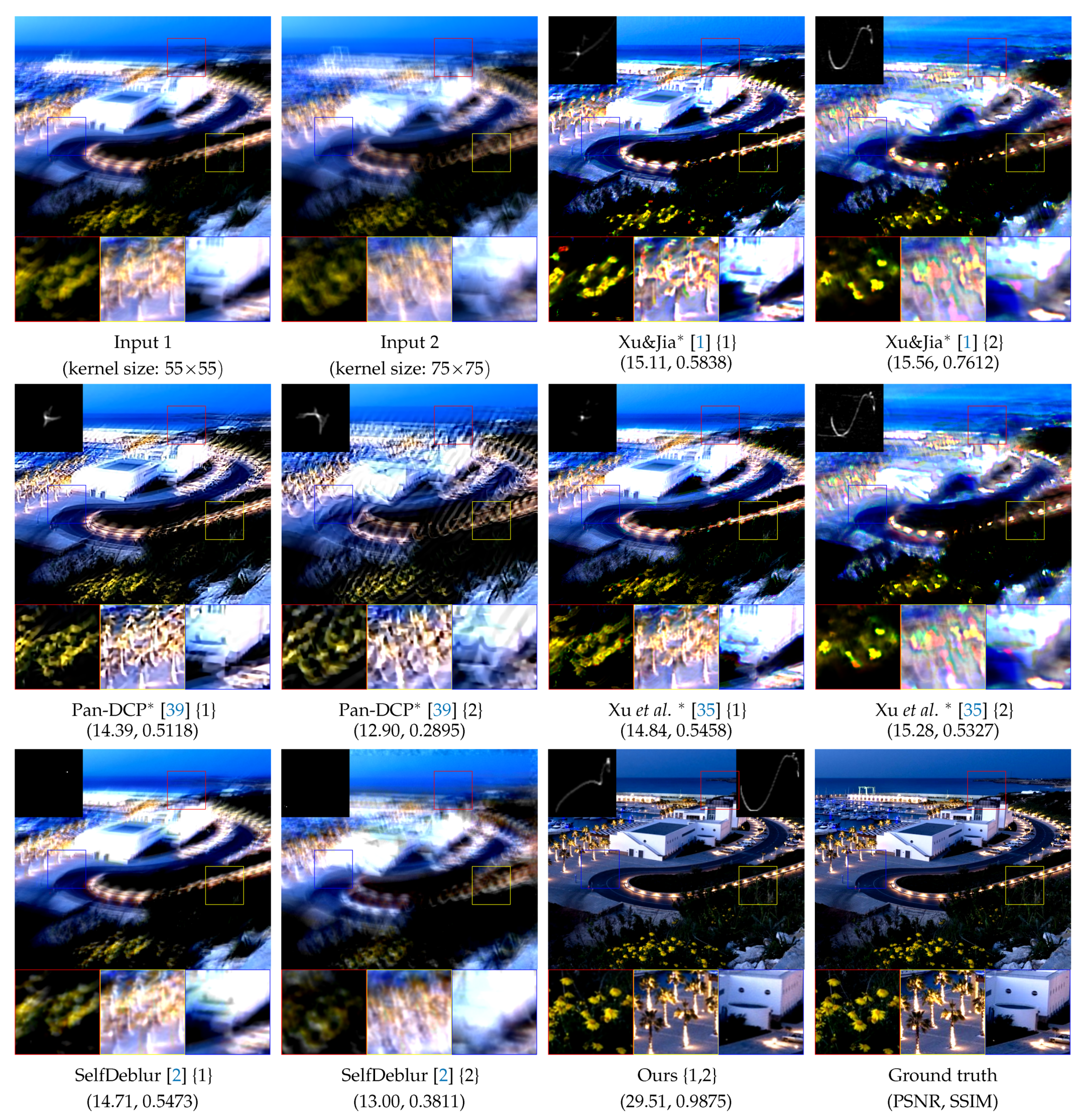
4.4. Comparison on Lai Test Set

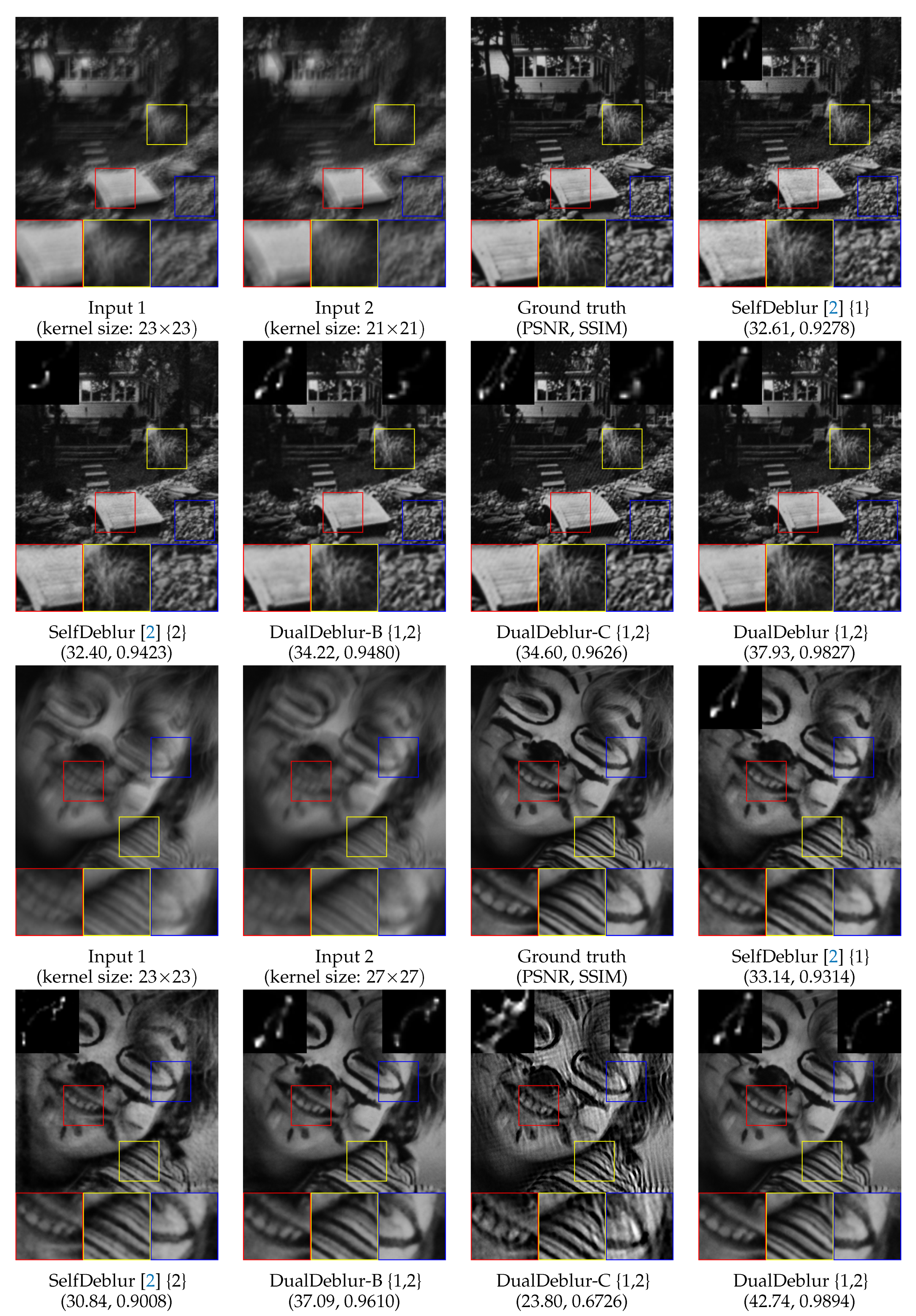
For the Lai test set [45], our method was compared with those of Cho and Lee [30], Xu and Jia [21], Xu et al. [35], Michael et al. [38], Perrone et al. [27], Pan-DCP [39], and SelfDeblur [18]. In previous methods, after blur kernel estimation, ref. [47] was applied to the $Saturated$ category as deconvolution, and ref. [31] to the other categories. In

Table 6. Quantitative comparisons on the Lai test set [45]. The methods marked with * adopt [31,47] as non-blind deconvolution for the final result after kernel estimation. Ref. [47] is adopted as a non-blind deconvolution method in the $Saturated$ category, and ref. [31] for the other categories. The best results are highlighted. Results of the blur kernel “Avg.” means the averagePSNR, SSIM, FSIM and LPIPS results for all blur kernels.

Method	Blur Kernel	PSNR ↑	SSIM ↑	FSIM ↑	LPIPS ↓	Method	Blur Kernel	PSNR ↑	SSIM ↑	FSIM ↑	LPIPS ↓
Cho & Lee * [30]	31	19.60	0.6664	0.7182	0.3855	Cho & Lee * [30]	51	16.74	0.4342	0.6394	0.4996
Xu & Jia * [21]	31	23.70	0.8534	0.8069	0.3099	Xu & Jia * [21]	51	19.69	0.6821	0.6773	0.3982
Xu et al. * [35]	31	22.90	0.8077	0.7928	0.3151	Xu et al. * [35]	51	19.18	0.6603	0.6703	0.4073
Michaeli et al. * [38]	31	22.02	0.7499	07668	0.3492	Michaeli et al. * [38]	51	18.07	0.4995	0.6562	0.4791
Perrone et al. * [27]	31	22.12	0.8279	0.7562	0.3501	Perrone et al. * [27]	51	16.21	0.4471	0.6358	0.5002
Pan-L0 * [36]	31	22.58	0.8405	0.7886	0.3267	Pan-L0 * [36]	51	18.08	0.6233	0.6637	0.4271
Pan-DCP * [39]	31	23.38	0.8478	0.8029	0.3580	Pan-DCP * [39]	51	19.69	0.6961	0.6736	0.4475
SelfDeblur [18]	31	22.40	0.8345	0.8005	0.4205	SelfDeblur [18]	51	21.27	0.7748	0.7928	0.4708
Ours (hard)	31, 51	28.57	0.9711	0.8056	0.1959	Ours (soft)	51, 55	28.32	0.9598	0.8034	0.2131
Ours (hard)	31, 75	29.09	0.9751	0.8276	0.1691	Ours (hard)	51, 75	28.78	0.9613	0.8252	0.1781
Method	Blur Kernel	PSNR↑	SSIM↑	FSIM↑	LPIPS↓	Method	Blur Kernel	PSNR↑	SSIM↑	FSIM↑	LPIPS↓
Cho & Lee * [30]	55	16.99	0.4857	0.6581	0.4863	Cho & Lee * [30]	Avg.	17.06	0.4801	0.6571	0.4997
Xu & Jia * [21]	55	18.98	0.6454	0.6794	0.4179	Xu & Jia * [21]	Avg.	20.18	0.7080	0.7123	0.4121
Xu et al. * [35]	55	18.12	0.5859	0.6707	0.4386	Xu et al. * [35]	Avg.	19.23	0.6593	0.6971	0.4278
Michaeli et al. * [38]	55	17.66	0.4945	0.6554	0.4942	Michaeli et al. * [38]	Avg.	18.37	0.5181	0.6729	0.4904
Perrone et al. * [27]	55	17.33	0.5607	0.6657	0.4545	Perrone et al. * [27]	Avg.	18.48	0.6130	0.6887	0.4568
Pan-L0 * [36]	55	17.19	0.5367	0.6542	0.4602	Pan-L0 * [36]	Avg.	18.54	0.6248	0.6888	0.4454
Pan-DCP * [39]	55	18.71	0.6136	0.6637	0.4520	Pan-DCP * [39]	Avg.	19.89	0.6656	0.6987	0.4625
SelfDeblur [18]	55	20.84	0.7590	0.7017	0.5112	SelfDeblur [18]	Avg.	20.97	0.7524	0.7488	0.5076
Ours (hard)	55, 75	28.72	0.9624	0.8337	0.1813	Ours (average)	Avg.	28.69	0.9660	0.8191	0.1875

, our DualDeblur results achieved better quantitative metrics, compared with the previous methods. Our average results for the Lai test set [45] were 7.72 higher for PSNR and 0.2136 higher for SSIM compared with the 2nd highest SelfDelbur [18]. The results of LPIPS showed that our method can restore more perceptually high-quality images, compared to other methods. Additionally, our method performed superior for all blur kernels. This shows that the proposed DualDeblur method performed excellently for large and diverse images. Both our soft and hard pairs outperformed the results of the previous methods.

In Figure 4 and Figure 5, through a qualitative comparison, it can be seen that our DualDeblur is visually superior to the previous methods. The kernel estimated by our DualDeblur is highly accurate compared with the other methods. Although other methods suffer from blur or ringing artifacts, our results are perceivably superior with rich texture (see Figure 4 details). Additionally, Figure 5 shows the high-quality details of our result; clearly, only the result of our method accurately reconstructs the stripes of the tie.

In Figure 6, our method shows superior results when using two blurry images that cannot be deblurred by the previous methods. Conversely, our method performs deblurring by jointly using two blurred images that are severely damaged and contain little information. In the 3rd line of Figure 6, SelfDeblur [18] fails to estimate the blur kernels in both input 1 and input 2, whereas our method is superior in estimating the blur kernels and the final image.

4.5. Ablation Study

To investigate the effectiveness of the proposed dual architecture and adaptive $L_2\_$SSIM loss, we conducted ablation studies. After equalizing the loss, we compared the dual architecture (called DualDeblur-A) with [18] to investigate the effect of the dual architecture. Furthermore, we demonstrated the effectiveness of our adaptive $L_2\_$SSIM loss by comparing models optimized using $L_{L_2\_SSIM}$ and only $L_2$ or $L_{SSIM}$. Models DualDeblur-B and DualDeblur-C have the same architecture as DualDeblur-A; however, DualDeblur-B uses only $L_2$ in Equation (3) and DualDeblur-C uses only $L_{SSIM}$ in Equation (4) for optimization. Finally, we define DualDeblur, using the proposed $L_{L_2\_SSIM}$ in Equation (5). The quantitative and qualitative comparisons are shown in

Table 7. Ablation study on the Levin test set [33]. The best results are highlighted.

Approach	Loss Fn.	PSNR ↑	SSIM ↑	Error Ratio ↓	FSIM ↑	LPIPS ↓
(a) SelfDeblur [18]	$L_2$ + TV	33.07	0.9438	1.2509	0.8086	0.1082
(b) DualDeblur-A	$L_2$ + TV	35.75	0.9536	0.6921	0.8824	0.0748
(c) DualDeblur-B	$L_2$	35.63	0.9528	0.7087	0.8816	0.0758
(d) DualDeblur-C	$L_{SSIM}$	39.11	0.9661	0.6226	0.7890	0.0819
(e) DualDeblur	$L_{L_2\_SSIM}$	40.89	0.9873	0.3798	0.8627	0.0461

and Figure 7, respectively.

4.5.1. Effects of Dual Architecture

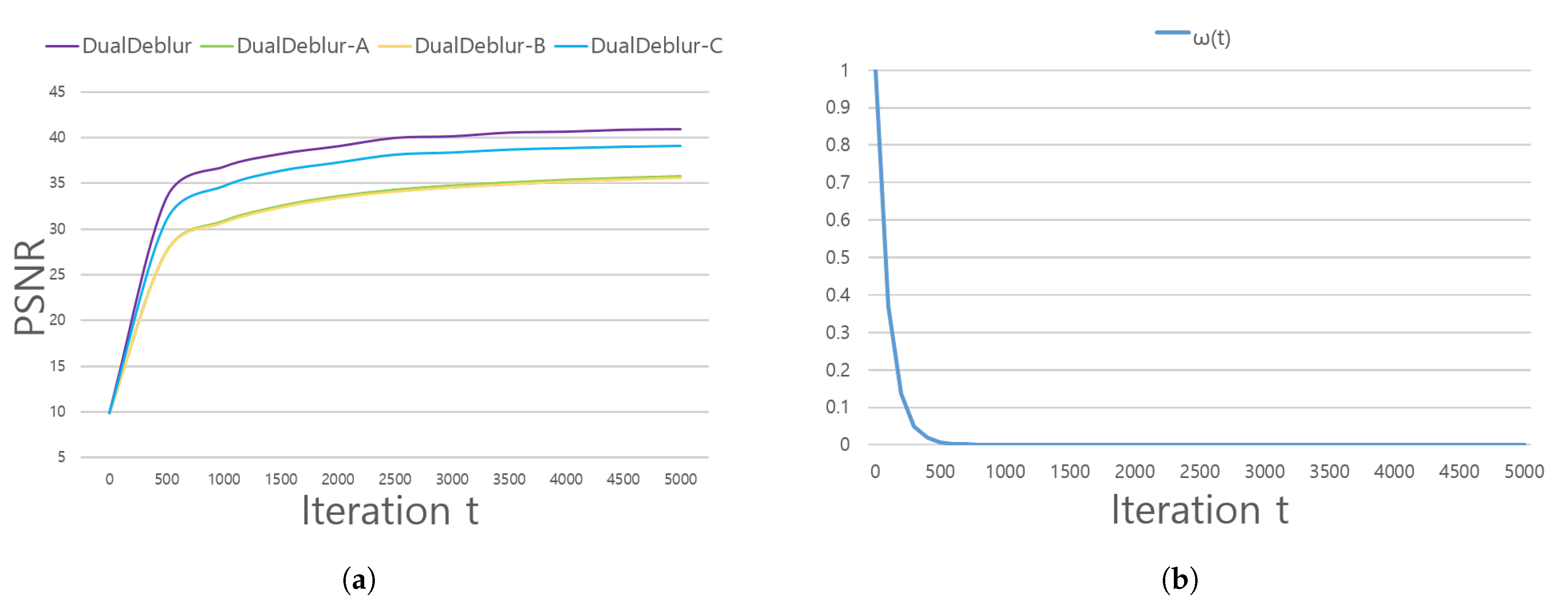
Unlike SelfDeblur [18], which performs deblurring with a single observation, our method leverages multiple observations via a dual architecture. In our experiments, DualDeblur-A using a dual architecture significantly improved the deblurring performance, compared to SelfDeblur (see (a) and (b) in Table 7). The PSNR and SSIM results of DualDeblur-A increased by 2.68 and 0.0098, respectively, compared to those of SelfDeblur. For FSIM and LPIPS, the results of DualDeblur-A are also better than those of SelfDeblur by 0.738 and 0.0334, respectively. This indicates that using multiple images is more helpful for deblurring than using a single image. This also shows that the proposed method is effective in handling multiple images during the deblurring procedure. The results of DualDeblur-A and DualDeblur-B (see Table 7) show that the performance of DualDeblur-B without TV regularization is similar to that of DualDeblur-A. These results show that the dual architecture works well without an additional regularizer.

4.5.2. Effects of Adaptive $L_2$_SSIM Loss

The proposed adaptive $L_2\_$SSIM loss, formulated as the weighted sum of $L_2$ and $L_{SSIM}$, focuses on restoring the intensity values per pixel first and then gradually restoring the structure later. By using the proposed adaptive $L_2\_$SSIM loss, we aim to exploit the advantages of $L_2$ and $L_{SSIM}$ loss functions and complement their limitations. To demonstrate the effectiveness of the adaptive $L_2\_$SSIM loss, we compare the performances of DualDeblur optimized with various loss functions (1) DualDeblur-B using the $L_2$ loss, (2) DualDeblur-C using the $L_{SSIM}$ loss, and (3) DualDeblur using the $L_{L_2\_SSIM}$ loss.

When optimizing our model using only the $L_2$ loss, the quantitative results are the worst in PSNR and SSIM (see Table 7). As shown in Figure 7, the results of our method using only the $L_2$ loss are overly smooth and fail to restore the details. To overcome this, we employed the structural loss ($L_{SSIM}$) in our method to enhance the perceptual quality and structural details in local regions [48]. Figure 7 also shows that using $L_{SSIM}$ helps restore details of the image rather than using only the $L_2$ loss. However, $L_{SSIM}$ does not restore the accurate pixel intensity. Additionally, corrupted structures in blurry observations may lead to unexpected structures in the resulting images.

However, in Figure 7 the results of our adaptive $L_2\_$SSIM loss $L_{L_2\_SSIM}$ demonstrate not only effectiveness in restoring accurate pixel values, but also in restoring the details and sharp edges of the image. As shown in Table 7, DualDeblur achieves the best in most metrics including PSNR, SSIM, and LPIPS except FSIM. Specifically, the results of DualDeblur show that the average PSNR increases by 5.26 and 1.78, compared with those of DualDeblur-B and DualDeblur-C, respectively. In addition, the results of DualDeblur show that the average SSIM is 0.0212 higher than the second-highest DualDeblur-C, that the average FSIM is 0.0197 lower than the highest DaulDeblur-A, and that the average LPIPS is 0.0287 better than the second-best DualDeblur-A. Figure 8a demonstrates the effectiveness of our adaptive $L_2\_$SSIM loss. The proposed adaptive $L_2\_$SSIM loss outperforms all other losses in every iteration. Figure 8b shows the change of $\omega \left(t\right)$ in Equation (5), which is the weight of the adaptive $L_2\_$SSIM loss following the training iterations. As mentioned earlier, the $L_2$ is more weighted than $L_{SSIM}$ in the initial iteration step, and the weight of $L_{SSIM}$ increases exponentially.

As shown in

Table 8. Influence of $\alpha$ and $\gamma$ in Equation (5) on the Levin test set [33]. The best results are highlighted.

$\mathit{\alpha }$	$\mathit{\gamma }$	PSNR ↑	SSIM ↑	FSIM ↑	LPIPS
1	10	38.85	0.9649	0.7770	0.0870
1	100	39.69	0.9766	0.7904	0.0780
1	200	40.65	0.9858	0.8126	0.0660
10	10	39.77	0.9799	0.8073	0.0684
10	100	40.89	0.9873	0.8627	0.0461
10	200	40.70	0.9872	0.8592	0.0487
50	10	39.33	0.9826	0.8610	0.0514
50	100	39.27	0.9818	0.8756	0.0465
50	200	38.96	0.9805	0.8784	0.0459

, we conduct various experiments on the $\alpha$ and $\gamma$ of Equation (5). The results show that the model with $\alpha =10$ and $\gamma =100$ gives the best results for both PSNR and SSIM, whereas the model with $\alpha =50$ and $\gamma =200$ is the best for FSIM and LPIPS. We select the model with $\alpha =10$ and $\gamma =100$ because PSNR and SSIM are the most commonly used metrics.

5. Conclusions

In this paper, we proposed a DualDeblur framework to restore a single sharp image using multiple blurry images. Our framework adopted a dual architecture to utilize the complementary information of two blurry images for obtaining a single sharp image. We proposed an adaptive $L_2\_$SSIM loss to ensure both pixel accuracy and structural details. For practical and accurate performance evaluation of our results, we divided the blur pairs into soft and hard pairs. Extensive comparisons demonstrated the superior results of our DualDeblur, compared to those of previous methods in both quantitative and qualitative evaluations.

References

1. Simonyan, K.; Zisserman, A. Very deep convolutional networks for large-scale image recognition. arXiv 2014, arXiv:1409.1556. [Google Scholar]
2. He, K.; Zhang, X.; Ren, S.; Sun, J. Deep residual learning for image recognition. In Proceedings of the IEEE Conference on Computer Vision and Pattern Recognition, Las Vegas, NV, USA, 27–30 June 2016; pp. 770–778. [Google Scholar]
3. Hu, J.; Shen, L.; Sun, G. Squeeze-and-excitation networks. In Proceedings of the IEEE Conference on Computer Vision and Pattern Recognition, Salt Lake City, UT, USA, 18–22 June 2018; pp. 7132–7141. [Google Scholar]
4. Girshick, R. Fast r-cnn. In Proceedings of the IEEE International Conference on Computer Vision, Santiago, Chile, 11–16 December 2015; pp. 1440–1448. [Google Scholar]
5. He, K.; Gkioxari, G.; Dollár, P.; Girshick, R. Mask r-cnn. In Proceedings of the IEEE International Conference on Computer Vision, Venice, Italy, 22–29 October 2017; pp. 2961–2969. [Google Scholar]
6. Redmon, J.; Divvala, S.; Girshick, R.; Farhadi, A. You only look once: Unified, real-time object detection. In Proceedings of the IEEE Conference on Computer Vision and Pattern Recognition, Las Vegas, NV, USA, 27–30 June 2016; pp. 779–788. [Google Scholar]
7. Ronneberger, O.; Fischer, P.; Brox, T. U-net: Convolutional networks for biomedical image segmentation. In International Conference on Medical Image Computing and Computer-Assisted Intervention; Springer: Berlin/Heidelberg, Germany, 2015; pp. 234–241. [Google Scholar]
8. Chen, L.C.; Papandreou, G.; Kokkinos, I.; Murphy, K.; Yuille, A.L. Deeplab: Semantic image segmentation with deep convolutional nets, atrous convolution, and fully connected crfs. IEEE Trans. Pattern Anal. Mach. Intell. 2017, 40, 834–848. [Google Scholar] [CrossRef] [PubMed]
9. Wang, Z.; Bovik, A.C.; Sheikh, H.R.; Simoncelli, E.P. Image quality assessment: From error visibility to structural similarity. IEEE Trans. Image Process. 2004, 13, 600–612. [Google Scholar] [CrossRef] [PubMed] [Green Version]
10. Nah, S.; Hyun Kim, T.; Mu Lee, K. Deep multi-scale convolutional neural network for dynamic scene deblurring. In Proceedings of the IEEE Conference on Computer Vision and Pattern Recognition, Honolulu, HI, USA, 21–26 July 2017; pp. 3883–3891. [Google Scholar]
11. Su, S.; Delbracio, M.; Wang, J.; Sapiro, G.; Heidrich, W.; Wang, O. Deep video deblurring for hand-held cameras. In Proceedings of the IEEE Conference on Computer Vision and Pattern Recognition, Honolulu, HI, USA, 21–26 July 2017; pp. 1279–1288. [Google Scholar]
12. Tao, X.; Gao, H.; Shen, X.; Wang, J.; Jia, J. Scale-recurrent network for deep image deblurring. In Proceedings of the IEEE Conference on Computer Vision and Pattern Recognition, Salt Lake City, UT, USA, 18–22 June 2018; pp. 8174–8182. [Google Scholar]
13. Zhang, J.; Pan, J.; Ren, J.; Song, Y.; Bao, L.; Lau, R.W.; Yang, M.H. Dynamic scene deblurring using spatially variant recurrent neural networks. In Proceedings of the IEEE Conference on Computer Vision and Pattern Recognition, Salt Lake City, UT, USA, 18–22 June 2018; pp. 2521–2529. [Google Scholar]
14. Zhang, H.; Dai, Y.; Li, H.; Koniusz, P. Deep stacked hierarchical multi-patch network for image deblurring. In Proceedings of the IEEE Conference on Computer Vision and Pattern Recognition, Long Beach, CA, USA, 16–20 June 2019; pp. 5978–5986. [Google Scholar]
15. Zamir, S.W.; Arora, A.; Khan, S.; Hayat, M.; Khan, F.S.; Yang, M.H.; Shao, L. Multi-stage progressive image restoration. arXiv 2021, arXiv:2102.02808. [Google Scholar]
16. Quan, Y.; Chen, M.; Pang, T.; Ji, H. Self2self with dropout: Learning self-supervised denoising from single image. In Proceedings of the IEEE Conference on Computer Vision and Pattern Recognition, Seattle, WA, USA, 13–19 June 2020; pp. 1890–1898. [Google Scholar]
17. Ulyanov, D.; Vedaldi, A.; Lempitsky, V. Deep image prior. In Proceedings of the IEEE Conference on Computer Vision and Pattern Recognition, Salt Lake City, UT, USA, 18–22 June 2018; pp. 9446–9454. [Google Scholar]
18. Ren, D.; Zhang, K.; Wang, Q.; Hu, Q.; Zuo, W. Neural blind deconvolution using deep priors. In Proceedings of the IEEE Conference on Computer Vision and Pattern Recognition, Seattle, WA, USA, 13–19 June 2020; pp. 3341–3350. [Google Scholar]
19. Zhang, H.; Wipf, D.; Zhang, Y. Multi-image blind deblurring using a coupled adaptive sparse prior. In Proceedings of the IEEE Conference on Computer Vision and Pattern Recognition, Portland, OR, USA, 23–27 June 2013; pp. 1051–1058. [Google Scholar]
20. Rav-Acha, A.; Peleg, S. Two motion-blurred images are better than one. Pattern Recognit. Lett. 2005, 26, 311–317. [Google Scholar] [CrossRef]
21. Xu, L.; Jia, J. Two-phase kernel estimation for robust motion deblurring. In European Conference on Computer Vision; Springer: Berlin/Heidelberg, Germany, 2010; pp. 157–170. [Google Scholar]
22. Wang, Z.; Simoncelli, E.P.; Bovik, A.C. Multiscale structural similarity for image quality assessment. In Proceedings of the Thrity-Seventh Asilomar Conference on Signals, Systems & Computers, Pacific Grove, CA, USA, 9–12 November 2003; 2003; Volume 2, pp. 1398–1402. [Google Scholar]
23. Zhang, L.; Zhang, L.; Mou, X.; Zhang, D. FSIM: A feature similarity index for image quality assessment. IEEE Trans. Image Process. 2011, 20, 2378–2386. [Google Scholar] [CrossRef] [PubMed] [Green Version]
24. Wang, H.; Yue, Z.; Zhao, Q.; Meng, D. A Deep Variational Bayesian Framework for Blind Image Deblurring. arXiv 2021, arXiv:2106.02884. [Google Scholar]
25. Krizhevsky, A.; Sutskever, I.; Hinton, G.E. Imagenet classification with deep convolutional neural networks. Adv. Neural Inf. Process. Syst. 2012, 25, 1097–1105. [Google Scholar] [CrossRef]
26. Chan, T.F.; Wong, C.K. Total variation blind deconvolution. IEEE Trans. Image Process. 1998, 7, 370–375. [Google Scholar] [CrossRef] [PubMed] [Green Version]
27. Perrone, D.; Favaro, P. Total variation blind deconvolution: The devil is in the details. In Proceedings of the IEEE Conference on Computer Vision and Pattern Recognition, Columbus, OH, USA, 23–28 June 2014; pp. 2909–2916. [Google Scholar]
28. Fergus, R.; Singh, B.; Hertzmann, A.; Roweis, S.T.; Freeman, W.T. Removing camera shake from a single photograph. In ACM SIGGRAPH 2006 Papers; Association for Computing Machinery: New York, NY, USA, 2006; pp. 787–794. [Google Scholar]
29. Zuo, W.; Ren, D.; Zhang, D.; Gu, S.; Zhang, L. Learning iteration-wise generalized shrinkage–thresholding operators for blind deconvolution. IEEE Trans. Image Process. 2016, 25, 1751–1764. [Google Scholar] [CrossRef]
30. Cho, S.; Lee, S. Fast motion deblurring. In ACM SIGGRAPH Asia 2009 Papers; Association for Computing Machinery: New York, NY, USA, 2009; pp. 1–8. [Google Scholar]
31. Krishnan, D.; Fergus, R. Fast image deconvolution using hyper-Laplacian priors. Adv. Neural Inf. Process. Syst. 2009, 22, 1033–1041. [Google Scholar]
32. Krishnan, D.; Tay, T.; Fergus, R. Blind deconvolution using a normalized sparsity measure. In Proceedings of the IEEE Conference on Computer Vision and Pattern Recognition, Colorado Springs, CO, USA, 20–25 June 2011; pp. 233–240. [Google Scholar]
33. Levin, A.; Weiss, Y.; Durand, F.; Freeman, W.T. Understanding and evaluating blind deconvolution algorithms. In Proceedings of the IEEE Conference on Computer Vision and Pattern Recognition, Miami, FL, USA, 20–25 June 2009; pp. 1964–1971. [Google Scholar]
34. Levin, A.; Weiss, Y.; Durand, F.; Freeman, W.T. Efficient marginal likelihood optimization in blind deconvolution. In Proceedings of the IEEE Conference on Computer Vision and Pattern Recognition, Colorado Springs, CO, USA, 20–25 June 2011; pp. 2657–2664. [Google Scholar]
35. Xu, L.; Zheng, S.; Jia, J. Unnatural l0 sparse representation for natural image deblurring. In Proceedings of the IEEE Conference on Computer Vision and Pattern Recognition, Portland, OR, USA, 23–28 June 2013; pp. 1107–1114. [Google Scholar]
36. Pan, J.; Hu, Z.; Su, Z.; Yang, M.H. l_0-regularized intensity and gradient prior for deblurring text images and beyond. IEEE Trans. Pattern Anal. Mach. Intell. 2016, 39, 342–355. [Google Scholar] [CrossRef] [PubMed]
37. Sun, L.; Cho, S.; Wang, J.; Hays, J. Edge-based blur kernel estimation using patch priors. In Proceedings of the IEEE International Conference on Computational Photography, Cambridge, MA, USA, 19–21 April 2013; pp. 1–8. [Google Scholar]
38. Michaeli, T.; Irani, M. Blind deblurring using internal patch recurrence. In European Conference on Computer Vision; Springer: Berlin/Heidelberg, Germany, 2014; pp. 783–798. [Google Scholar]
39. Pan, J.; Sun, D.; Pfister, H.; Yang, M.H. Deblurring images via dark channel prior. IEEE Trans. Pattern Anal. Mach. Intell. 2017, 40, 2315–2328. [Google Scholar] [CrossRef] [PubMed]
40. Sun, J.; Cao, W.; Xu, Z.; Ponce, J. Learning a convolutional neural network for non-uniform motion blur removal. In Proceedings of the IEEE Conference on Computer Vision and Pattern Recognition, San Diego, CA, USA, 7–9 May 2015; pp. 769–777. [Google Scholar]
41. Chakrabarti, A. A neural approach to blind motion deblurring. In European Conference on Computer Vision; Springer: Berlin/Heidelberg, Germany, 2016; pp. 221–235. [Google Scholar]
42. Sajjadi, M.S.; Scholkopf, B.; Hirsch, M. Enhancenet: Single image super-resolution through automated texture synthesis. In Proceedings of the IEEE International Conference on Computer Vision, Honolulu, HI, USA, 21–26 July 2017; pp. 4491–4500. [Google Scholar]
43. Zhang, R.; Isola, P.; Efros, A.A.; Shechtman, E.; Wang, O. The unreasonable effectiveness of deep features as a perceptual metric. In Proceedings of the IEEE Conference on Computer Vision and Pattern Recognition, Salt Lake City, UT, USA, 18–22 June 2018; pp. 586–595. [Google Scholar]
44. Kingma, D.P.; Ba, J. Adam: A method for stochastic optimization. arXiv 2014, arXiv:1412.6980. [Google Scholar]
45. Lai, W.S.; Huang, J.B.; Hu, Z.; Ahuja, N.; Yang, M.H. A comparative study for single image blind deblurring. In Proceedings of the IEEE Conference on Computer Vision and Pattern Recognition, Las Vegas, NV, USA, 27–30 June 2016; pp. 1701–1709. [Google Scholar]
46. Paszke, A.; Gross, S.; Massa, F.; Lerer, A.; Bradbury, J.; Chanan, G.; Killeen, T.; Lin, Z.; Gimelshein, N.; Antiga, L.; et al. PyTorch: An Imperative Style, High-Performance Deep Learning Library. Adv. Neural Inf. Process. Syst. 2019, 32, 8026–8037. [Google Scholar]
47. Whyte, O.; Sivic, J.; Zisserman, A. Deblurring shaken and partially saturated images. Int. J. Comput. Vis. 2014, 110, 185–201. [Google Scholar] [CrossRef]
48. Zhao, H.; Gallo, O.; Frosio, I.; Kautz, J. Loss functions for image restoration with neural networks. IEEE Trans. Comput. Imaging 2016, 3, 47–57. [Google Scholar] [CrossRef]
Figure 1. Visual quality comparison. The input image for each method is denoted as { } (i.e., ours {1,2} indicates our resulting image when the input images are blurry image 1 and blurry image 2). (a) Ground-truth image. (b) Blurry image with kernel size 55 × 55. (c) Blurry image with kernel size 75 × 75. (d,e) Results of [21] corresponding to (b,c), respectively. In (d), PSNR is 15.33 and in (e), PSNR is 14.45. (f,g) Results of [18] corresponding to (b,c), respectively. In (f), PSNR is 21.03 and in (g), PSNR is 20.15. (h) Our result. In (h), PSNR is 26.82.
Electronics 10 02045 g001
Figure 2. Architecture of the proposed DualDeblur.
Electronics 10 02045 g002
Figure 3. Qualitative comparisons on the Levin test set [33]. * indicates that the method uses the non-blind deconvolution method of [34] to produce the final result. The input image for each method is denoted as { } (i.e., ours {1,2} indicates our resulting image when the input images are input 1 and input 2).
Electronics 10 02045 g003
Figure 4. Qualitative comparisons on the Lai test set [45]. * indicates that the method uses the non-blind deconvolution method of [34] to produce the final result. The input image for each method is denoted as { } (i.e., ours {1,2} indicates our resulting image when the input images are input 1 and input 2).
Electronics 10 02045 g004
Figure 5. Qualitative comparisons on the Lai test set [45]. * indicates that the method uses the non-blind deconvolution method of [34] to produce the final result. The input image for each method is denoted as { } (i.e., ours {1,2} indicates our resulting image when the input images are input 1 and input 2).
Electronics 10 02045 g005
Figure 6. Qualitative comparisons on the Lai test set [45]. * indicates that the method uses the non-blind deconvolution method of [34] to produce the final result. The input image for each method is denoted as { } (i.e., ours {1,2} indicates our resulting image when the input images are input 1 and input 2).
Electronics 10 02045 g006
Figure 7. Ablation study. Qualitative comparisons on the Levin test set [33]. The input image for each method is denoted as { } (i.e., ours {1,2} indicates our resulting image when the input images are input 1 and input 2).
Electronics 10 02045 g007
Figure 8. (a) PSNR versus number of training iterations for ablation study. (b) Value of ω ( t ) versus number of training iterations.
Electronics 10 02045 g008