Analysis of Random Local Descriptors in Face Recognition

Abstract

This article describes and analyzes the new feature extraction technique, Random Local Descriptor (RLD), that is used for the Permutation Coding Neural Classifier (PCNC), and compares it with Local Binary Pattern (LBP-based) feature extraction. The paper presents a model of face feature detection using local descriptors, and describes an improvement on the PCNC for the recognition of plane rotated and small displaced face images, as applied to three databases, i.e., ORL, FRAV3D and FEI. All databases are described along with the recognition results that were obtained. We also include a comparison of our classifier with the Support Vector Machine (SVM) and Iterative Closest Point (ICP). The ORL database was selected to compare our RLDs with LBP-based algorithms. The PCNC with the RLDs demonstrated the best recognition rate, i.e., 97.49%, in comparison with 90.49% for LBPs. For the FEI image database, we obtained the best recognition rate, i.e., 93.57%, in comparison with 66.74% for LBPs. Using the RLDs and rotating the original images for FRAV3D, we improved the recognition rate by decreasing by approximately twice the number of errors. In addition, we analyzed the influence of different RLD parameters on the quality of facial recognition.

1. Introduction

Face recognition offers the advantage of being a passive identification and verification method that does not require explicit action or participation by the individual in order to be recognized. This characteristic makes this technique ideal for security and surveillance purposes. The acquisition methods for face images can be easily performed with inexpensive standard cameras at a long distance. However, unconstrained situations make it difficult to develop robust systems that are invariant to illumination, size, pose and location. Images in the real world are affected by expressions, poses, occlusions, and illumination; the differences among various face images of the same person could be even larger than those from images of a different person altogether. Therefore, extracting robust and discriminative features that make it possible to distinguish among different people is a critical and difficult problem in face recognition [1].

Automatic face recognition could be used in different security systems, such as security for buildings, offices and banks. Different approaches have been investigated and proposed for solving this task [2,3]. Face analysis systems are often built into mobile phones. Although the memory capabilities of mobile phones are limited, experiments show encouraging face detection performance.

Face recognition is a classical recognition process that involves two critical problems—feature representation and classifier construction [1]. It has been demonstratedthat different methods of feature extraction can be combined with different methods of classification in a handwritten digit recognition task.

The authors [4] consider that the design of effective features is a fundamental issue in computer vision. It is commonly accepted that designing effective features has an important tradeoff with discriminativeness and robustness.

The techniques developed thus far for face representation can be roughly classified into two main categories: holistic- and local-based techniques. Holistic approaches are based on the global use of the whole face region. Local-based techniques locate a number of features from a face and then classify them by combining and comparing them with corresponding local statistics. It has been proven that component-based (local feature-based) face recognition methods perform better than global methods (holistic-based).

Different face recognition systems, such as SpereFace, Arcface or Cosface, based on neural networks and deep learning, have been developed in recent years [5,6,7,8,9].

Here, we focus on aspects of feature extraction for facial recognition (classification) using local feature-based methods.

Recently, there has been substantial interest in object and view matching using local invariant features or local feature descriptors [1,4,10,11]. The methods that use these descriptors can be divided into two classes: sparse descriptors, which first detects the interest points in a given image and then samples a local patch and describes its invariant features [10]; and dense descriptors, which extract local features pixel by pixel.

As examples of sparse descriptors, we can mention scale-invariant feature transform (SIFT) and rotation-invariant feature transform (RIFT) [10,12]. A typical image of size 500 × 500 pixels gives rise to about 2000 stable features.

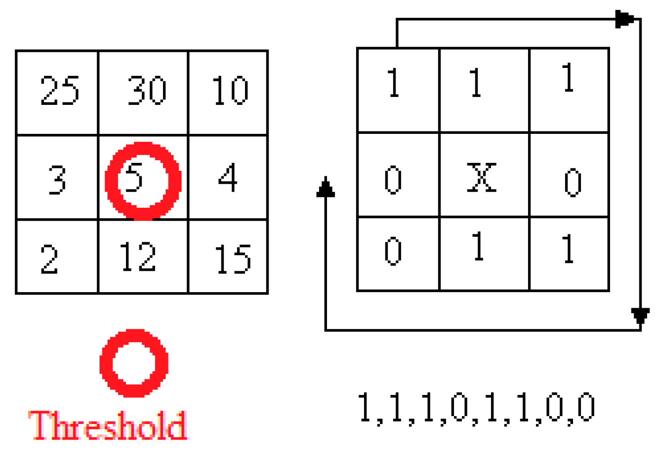
Examples of dense descriptors are Local Binary Pattern Descriptor (LBP) [13,14] and Weber Local Descriptor (WLD) [10]. LBP is one of the most powerful descriptors to represent local structures [13,14]. An example of a basic LBP operator is presented in Figure 1.

We have a window of 3 × 3 pixels in which every pixel has a brightness value, which is compared with the brightness of the central point. The value of the central point is a threshold. Each pixel is converted to a binary form of presentation in the following manner: If the brightness is more than the threshold, 1 is obtained; if the brightness is less than the threshold, 0 is obtained. The binary code of the window is formed from the left upper corner, as presented in Figure 1. Sometimes, the mean value of the window brightnesses is selected as a threshold for binary code calculations. LBP describes the micropattern on the image. It is possible to build an LBP histogram that is computed over the whole image. Such a representation encodes only the occurrences of micropatterns without any indication of their locations [15].

To use LBP for face recognition, it is necessary to divide face images into a grid of subregions. These subregions are not necessarily well aligned with facial features. Moreover, the resulting facial description depends on the chosen sizes and positions of these subregions [15]. The neighboring pixels in LBP could make different contributions to the description of the face. Careful selection of neighboring pixels could help to improve the face recognition performance [1]. In [15], researchers adopted a heuristic approach to find the best pixel sampling pairs in local regions. In [1], the authors proposed a soft method of determining the optimal neighborhood sampling strategy. They calculated the pixel difference vectors (PDV) in such way that the PDVs of images of the same person are similar, and the differences among different people are enlarged. One of the interesting conclusions of this work was that it used a local Discriminant Face Descriptor (DFD), which describes the face structures locally and precisely, and achieved better face recognition performance than global DFD [1]; the many experiments that were performed demonstrated this fact. It should be noted that with respect to computational cost, every image was divided into 49 nonoverlapping regions, each of which corresponded to a 1024-dimensional feature; therefore, the feature dimension of DFD was1024 × 49 = 50,176.

Ahonen et al. [13] introduced LBP in facial recognition with a nearest neighbor (NN) classifier.

In [1], the authors used cropped face examples from different image databases (e.g., FERET, LFW).

During the development of the LBP methodology, a large number of variations were designed to improve the performance or expand the applications; for example, ILBP (Improved LBP) and ELBP (Extended LBP) [15]. The downside of ELBP is that it significantly increases the feature dimensionality. The feature vector sometimes has a dimensionality range of 3540 to 10,620 in the case of colored images.

LBP-based features have a large dimensionality; to reduce this, this method is combined with some popular learning techniques which were developed and used for texture recognition, and then for face recognition tasks. Recent versions of UUCoLBP, RUCoLBP, and PRICoLBP were developed on the basis of LBP [4]. For example, PRICoLBP preserves pairwise rotation invariance.

The disadvantages of LBP are rarely discussed. However, LBP has sensitivity to random and quantization noise [15]. The development of a large number of LBP variations demonstrates the wish to avoid this problem and improve the performance in different applications [16,17]. However, these improvements typically increase the computational complexity.

The literature has proposed a combination of local face descriptors LBP/LDiP/LDNP with Discrete Fourier Transform (DFT) as a global face descriptor [18]. LDiP is Local Directional Pattern and LDNP is Local Directional Number Pattern. The results were obtained using the ORL database.

WLD [10] was inspired by Weber’s Law and is used as a robust local descriptor. The WLD method was tested on texture databases and demonstrated effective results. Forhuman face detection, this method also showed promising results with the use of an SVM classifier. Sometimes, the investigators used a WLD histogram for a given image [10].

Learning DFD was proposed in [1]. Traditionally, the form of such local descriptors is predefined in a hand-crafted way. This method proposes to learn a DFD in a data-driven way. A DFD introduces discriminant learning into the feature extraction process. The DFD was tested on different face databases and demonstrated improvements in the recognition results.

In this paper, we describe all of these local descriptors in detail to demonstrate the interest of scientists and engineers in the image recognition area, and in order to have examples with which to compare the advantages and disadvantages of these methods with the methods that we are proposing.

We have developed a special feature extractor and neural classifiers that we applied to different types of images, such as handwritten digit recognition, micro-object shape recognition, face recognition and other domains [19,20,21,22,23]. Different types of neural classifiers have been developed, for example, Random Threshold Classifier (RTC), Random Subspace Neural Classifier (RSC), Limited Receptive Area Classifier (LIRA classifier), etc.

The proposed feature extractor is based on the concept of random local descriptors (RLDs). RLDs are followed by an encoder that is based on the permutation coding technique, which accounts for not only the detected features, but also the position of each feature in the image, and makes the recognition process robust to small displacements. The combination of RLDs and permutation coding permits us to obtain a sufficiently general description of the image to be recognized. The code generated by the encoder is used as input data for the PCNC neural classifier.

In this article, we describe in detail the RLD and compare it with other local descriptors. We demonstrate the possibility of an RLD application for the face recognition task. From among several tasks, including face detection, face recognition, facial expression analysis, demographic classification (classification age, gender and ethnicity, based on face images) and other applications, we selected face recognition as an application for RLDs. We apply this RLD to face recognition using the different face image databases, for example, the ORL, FEI, and FRAV3D image databases.

The advantages of RLDs are that they can be easily extracted from the raw images to allow for fast processing, and they can be combined with a neural classifier to avoid computationally expensive algorithms.

The sizes and positions of RLDs can vary; they can overlap on the face image.

This paper focuses on the face recognition task. In previous studies (regarding the ORL database of faces), we proposed the inclusion of displaced face images as part of the training set and obtained a good recognition rate [22]. FEI [24] and the 2D images from the FRAV3D [25,26,27] databases fulfilled our investigation needs for the PCNC, and allowed us to obtain superior recognition rates. As we have the results of other authors for the ORL database and LBPs, we decided to repeat our experiments for ORL and RLDs in order to compare them.

An explanation of the PCNC classifier is given in Section 2. Section 3 provides a description of the ORL, FRAV3D and FEI databases, as well as the distortions that are included in the recognition process. In Section 4, we show the results of the experiments with the PCNC neural classifier in comparison with other face recognition algorithms, and present the new results of the experiments with the ORL and FEI databases. Concluding remarks are given in Section 5.

2. Permutation Coding Neural Classifier

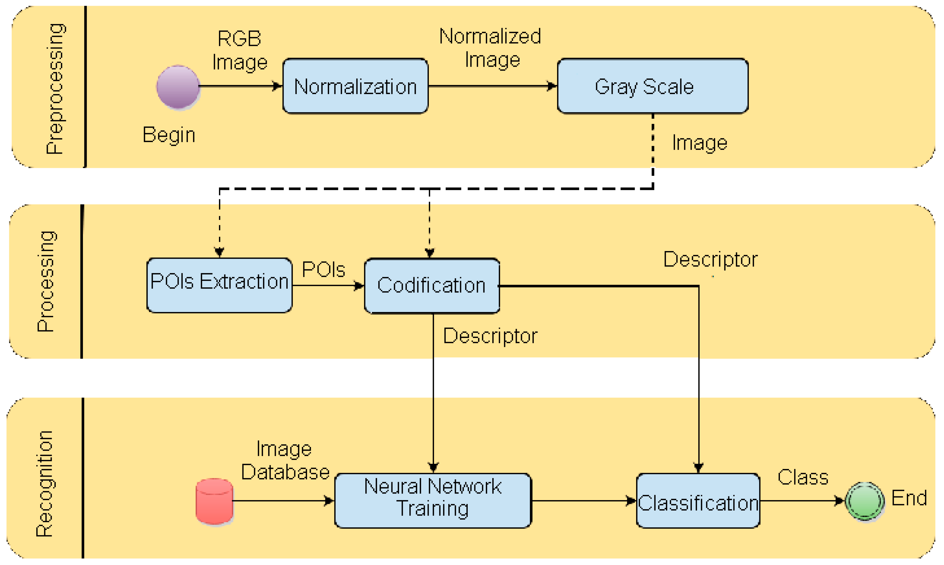
The PCNC is meant to be a multipurpose recognition tool. It has been tested on handwritten digits, micromechanical pieces and face recognition [20,21]. Figure 2 shows the processes that take place in the PCNC classifier.

As observed in Figure 2, there are three stages in the PCNC method: preprocessing, processing and recognition. The first stage, image preprocessing, converts color images to grayscale images. Sometimes, scientists use the color images in their investigations [28]. To reduce the complexity and determine the true invariance for face recognition, images can be converted from the RGB to gray scale, as described in [29]. In this paper, we used the equation

$$f(x,y)=(R+G+B)/3,$$

(1)

The gray-scale image was then processed with a median filter to obtain edges as points of interest (POIs in Figure 2).

The recognition stage includes two substages, i.e., training and recognition, for the recognition task with the PCNC classifier.

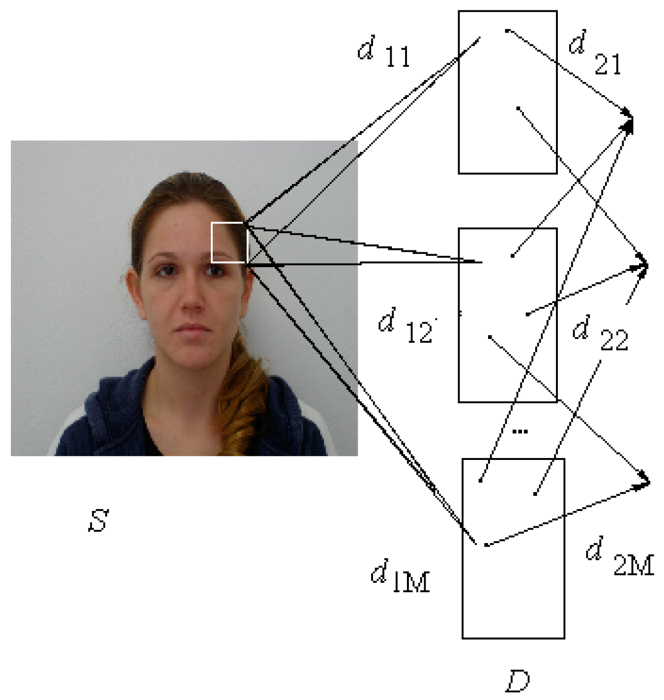
An example of extracting the POIs is demonstrated in Figure 3. The last image is used as the input image for our classifier.

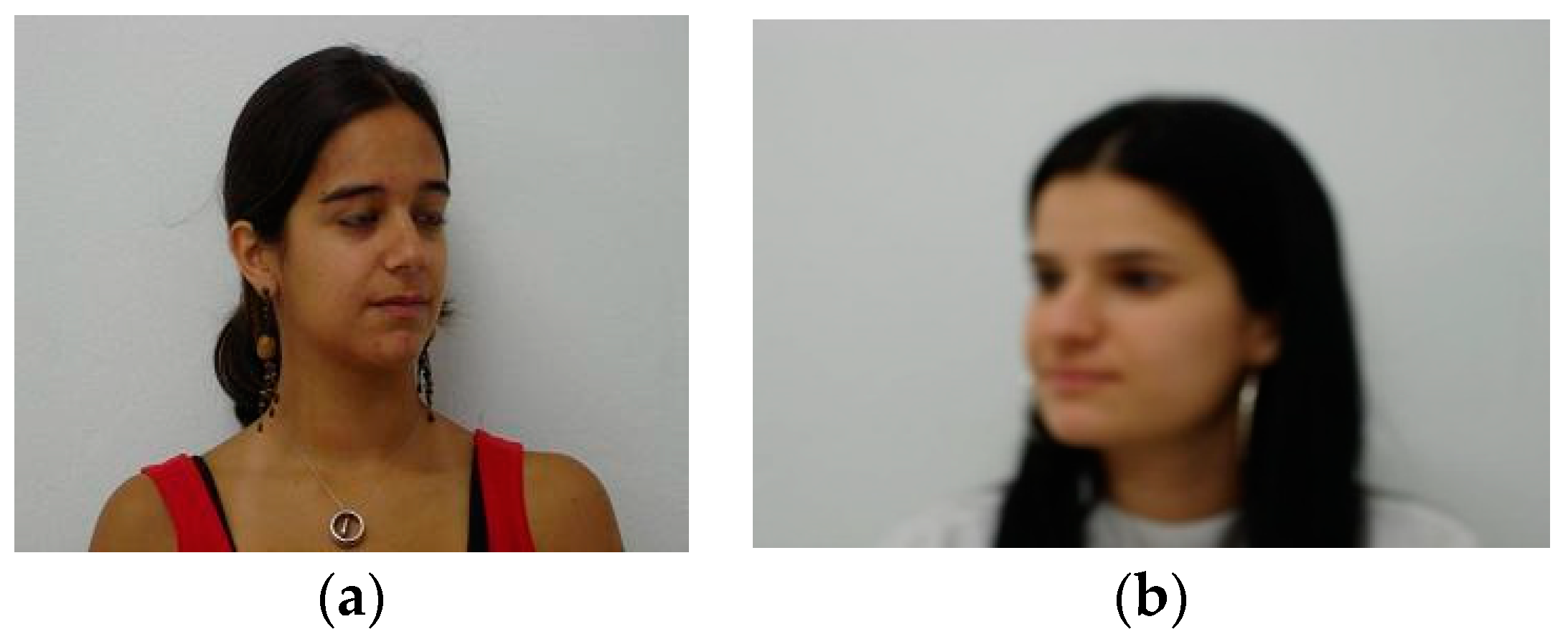
The resulting image from this stage is shown in Figure 4. The original image was taken from the FEI image database [24].

In face recognition, the feature representation of a face is the key to good performance. A good representation must minimize intraperson dissimilarities and maximize the differences among different people, as well as being fast and compact.

2.1. Extractor of Features

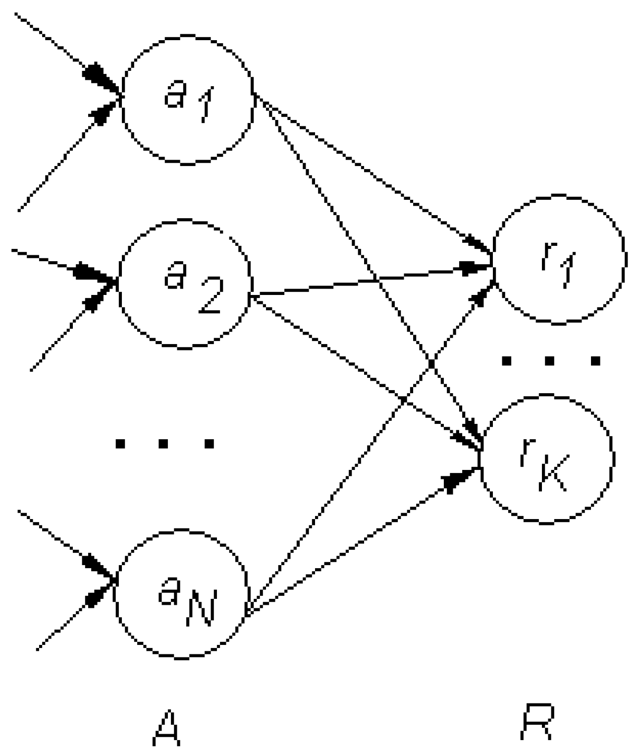
We propose a classifier using the concept of RLD and Frank Rosenblat’s perceptron [30]. RLD works as a general feature extractor by connecting a neuron in the associative layer to a random point in the retina (input image) and calculating a brightness function of the selected point. The scheme of the neural network recognition system is shown in Figure 5.

As shown in Figure 5, the system is based on a multilayer neural network. The first S layer (sensor layer) is the input image; the second D layer contains RLD neurons (Figure 6). The A layer is an associative layer of neurons (Figure 5). The R layer is an output layer. Each of these output neurons corresponds to a recognition image class. Here, we describe the RLD structure in detail.

The RLD scheme is presented in Figure 7. RLD is constructed around points of interest (POIs). The POI is in the center of the RLD (in Figure 7, the POI is not shown).

In this study, we assume that the POIs correspond to image locals in which the surface of the pixel brightness is not plain.

We collocate the RLD around the extracted POI. In the center of the scanning windows (h × w), there are two auxiliary rectangles: an internal rectangle with the area I × I = I² pixels, and an external rectangle with the area E × E = E² pixels (Figure 7). All of the pixels of the internal rectangle are connected with the neuron, with connections that have positive values for the weight being represented by w_I. All of the pixels of the external rectangle are connected to the neuron with the negative-valued weights, w_E. The weights w_I and w_E are selected according to the equation:

$$I^2\cdot w_I=E^2\cdot \left|w_E\right|,$$

(2)

The neuron calculates the input excitation:

$$E_{in}={\displaystyle \sum _{i=1}^I{\displaystyle \sum _{j=1}^I{b}_{ij}\cdot w_I-{\displaystyle \sum _{i=1}^E{\displaystyle \sum _{j=1}^E{b}_{ij}\cdot \left|w_E\right|}}}},$$

(3)

where $b_{ij}$ is the brightness of the pixel that has coordinates (i,j).

The neuron output equals 1 if

$$\left|E_{in}\right|\ge T,$$

(4)

where $T$ is the threshold. Otherwise, the neuron output equals 0.

For every RLD (Figure 7), two types of neurons are considered, similar to natural neural networks, namely, ON and OFF neurons (ON neurons correspond to pixels with a connection with the arrow or positive point; and OFF neurons correspond to pixels with a connection with the circle or negative point). ON neurons respond if the input is more than the threshold, whereas OFF neurons respond if the input is less than threshold. We use binary outputs, i.e., “1” (or active) and “0” (or inactive). In an image, these neurons correspond to the positive and negative points. Figure 8 presents an example of the RLD that determine each feature, which exists only when all of the ON and OFF neurons are active.

The ON neuron has an output of “1” if the brightness b_i of the corresponding pixel is higher than the neuron threshold T_i: b_i ≥ T_i.

The OFF neuron has an output of “1” if the brightness b_i of the corresponding pixel is less than the neuron threshold T_i: b_i < T_i.

The threshold values are randomly selected from among the brightness values T_min ≤ T_i ≤ T_max of the input image.

A D layer neuron (Figure 7) is a neuron that simulates a conjunction operation. It has an output of “1” if and only if all eight neurons (for connections with the arrow and four connections with circles) have outputs of “1”.

Each neuron of the d_ij plane (Figure 6) corresponds to the pixel that is located at the center of the I-rectangle (Figure 7).

All of the neurons that have an output of“1” are considered to be active neurons. We consider that the feature exists only if all of the positive and negative points are active; otherwise, it is absent.

All of the neurons of the associative A layer have trainable connections with R layer neurons (Figure 9). The training process is realized between these two layers by changing the weight of every connection between the A and R layers. If the answer is correct, nothing has been done. In the case of an incorrect answer, all connection weights to the incorrect neuron are reduced, and all weights to the correct neuron are increased.

2.2. Feature Encoder

To explain the feature encoder, we must introduce the following variables. Let a feature F_i be

$$F_i=(U_i,(P_{1}i,P_{2}i,\dots ,P_{k}i)),$$

(5)

where P_j is the position of the feature F_i in the image. We can have the same feature in different places of the image (for example, in Figure 10a, two white lines with the same inclination, or in Figure 10b, two different pairs of feature frames from the man’s lips).

Thus, for every feature, we can define the following:

$$P_j=\left(x_j,y_j,{\displaystyle \underset{1}{\overset{C}{\cap }}(O{N}_c,T{h}_{O{N}_c})},{\displaystyle \underset{1}{\overset{L}{\cap }}OF{F}_l,T{h}_{OF{F}_l}}\right),$$

(6)

where x_j and y_j are coordinates of the window of size (w × h) with a center in the point of interest, ${\displaystyle \underset{1}{\overset{C}{\cap }}(O{N}_c,T{h}_{O{N}_c})}$ is the conjunction function of C ON-neurons ($O{N}_c$ is the position of an ON-neuron randomly generated in window (w × h)), $T{h}_{O{N}_c}$ is the threshold of the c-th ON-neuron, ${\displaystyle \underset{1}{\overset{L}{\cap }}OF{F}_l,T{h}_{OF{F}_l}}$ is the conjunction function of L OFF-neurons ($OF{F}_l$ is the position of an OFF-neuron randomly generated in window (w × h)), and $T{h}_{OF{F}_l}$ is the threshold of the l-th OFF-neuron. A feature exists in the position (x_j, y_j) if the result of the conjunction for the ON and OFF neurons is 1. If one of these functions is 0, then the feature does not exist in that position.

To address all of these variables as $O{N}_c$ and $OF{F}_l$ neuron positions, the thresholds $T{h}_{O{N}_c}$ and $T{h}_{OF{F}_l}$ for the ON and OFF neurons are randomly selected.

The coordinates x_j and y_j of the center point of the window (w × h) are defined in the following manner. We scan the image with this window with a scan step of one pixel. If the central point is not a point of interest, we continue to scan the image. If the central point of the window is a point of interest, then we define the feature using Equation (7). If the result is 1 (i.e., all ON and OFF neurons have given an answer), then we know that the feature exists in this position. If the result is 0 (i.e., if at least one of the ON and OFF neurons does not give the answer), then we know that the feature is absent and we must continue to scan the image with the window.

For each extracted feature F_i, the encoder creates an auxiliary binary vector or mask, which is represented as follows:

$$U_i=(u_{i1},u_{i2},\dots ,u_{iN}),$$

(7)

where u_ii is equal to 0 or 1. U_i is the feature mask vector of dimension N with K 1’s, whose initial position is randomly chosen, where K<<N (we worked with K = 16 and N = 64,000). The mask corresponds to the feature in the initial position in the image and is constant throughout the lifetime of the PCNC. The other positions of the feature are encoded with permutations of the mask. Furthermore, we will describe in detail the permutation procedure. Next, we want to terminate the description of the coding procedure. As a result of the permutation process, a new vector $U_i(P_{z}i)$ is created. To code the presence of a feature in the image, we apply the disjunction operation to join all of the binary vectors of this feature in different places.

If Z be in different positions for the same feature F_i, the binary code will be

$$U_i={\displaystyle \underset{z=1}{\overset{Z}{\cup }}{U}_z(P_{z}i)},$$

(8)

where the vector $U_z$ is the feature mask binary vector of size N and $P_{z}i$ is the position of feature i that defines the permutations of the feature mask vector; thus, $U_z(P_{z}i)$ is the result of the feature mask vector permutation. N is a very large value.

Next, we explain the process of the permutation. The problem is to generate binary codes with special characteristics, i.e., the correlation between two binary vectors is a function of the distance between these two vectors. Thus, the permutation not only permits us to generate a unique code for every feature in its position, but also gives us the opportunity to analyze its correlation.

The number of permutations depends on the feature location in the image. Once the permutations of the binary vector U_z are completed, a new vector $U_z(P_{z}i)$ is created.

To code the position of the feature characteristic F_i, we must define the correlation distance D_c, which is the measurement between the feature distances (in our work, we use 16 pixels).

We are given two position points, P₁(x₁, y₁) and P₂(x₂, y₂), for feature F_i, the vectors $U_1(P_{1}i)$ and $U_2(P_{2}i)$, which code the feature for every position point, and dx, the Euclidian distance between P₁ and P₂ in X and dy in Y.

$$dx=abs(x_1-x_2);dy=abs(y_1-y_2),$$

(9)

The vectors $U_1(P_{1}i)$ and $U_2(P_{2}i)$ are correlated if dx < D_c or dy < D_c; otherwise, there is no correlation.

To code the feature F_m position, distance Dc is predefined, and the following values must be calculated:

$$X=x_{ij}/D_c,Y=y_{ij}/D_c.$$

(10)

We calculate the integer parts

$$E(X)=(\mathit{int})X,E(Y)=(\mathit{int})Y.$$

(11)

The integer parts correspond to the number of complete permutations of the feature mask binary vector. To evaluate the number of partial permutations, we must calculate the fractional parts of the feature coordinates. We obtain fractional parts from the following equations:

$$R(X)=x_{ij}-E(X)\cdot D_c,R(Y)=y_{ij}-E(Y)\cdot D_c,$$

(12)

$$P_x=\mathit{int}(R(X)\cdot N/D_c),P_y=\mathit{int}(R(Y)\cdot N/D_c),$$

(13)

where E(X) and E(Y) are the integer parts of X and Y; R(X) and R(Y)are the fractional parts of X and Y; y_ij is the vertical coordinate of the detected feature; x_ij is the horizontal coordinate of the detected feature; N is the number of neurons; E(X) and E(Y) show the number of permutations to perform in the X and Y directions; and P_x and P_y are the number of neurons in the range [0, N) for which an additional permutation is needed. The value of N is changed according to the problem complexity. In the case of facial recognition, we used 65,000 neurons.

The example permutation scheme for the X coordinate is presented in Figure 11 (we select E(X) = 2, and P_x = 2). The U vector is the binary vector. To more easily explain the permutation process, we use the letters that are contained in each element of the U vector. The process is performed as follows: each element from the first line is connected to a free and randomly selected element from the third line, using the permutation scheme presented in the second line (the A line). For example, 0 < −2 (0 “left arrow” 2) means that letter c from U(2) must be transported to U(0), and the scheme of the A line is used for all of the elements of the U vector. The third line is the result of the first permutation. The B line defines the second permutation, and the result is presented in the fourth line. The process repeats until all of the elements from the A line and B line end up with a one-to-one connection. In line C, only the two first elements have permutations (U(0) and U(1)), and the remaining elements do not change.

The full process of the feature extraction is shown in Figure 12.

The result of the feature extraction process is the associative vector A (binary vector or code), which equals a bitwise disjunction of all of the permutated vectors.

$$A={\displaystyle \underset{i}{\cup }{U}_i}.$$

(14)

3. Database and Distortions

3.1. ORL Database

One of the first databases for face recognition was ORL (Olivetti Research Laboratory), now administered by AT&T Laboratories Cambridge [31] (Figure 13). It has ten different images of each of 40 distinct subjects, and the original size of each image is 92 × 112 pixels. For some subjects, the images were taken at different times, varying the lighting, facial expressions (open/closed eyes, smiling/not smiling) and facial details (glasses/no glasses).

In the literature, many results were obtained using this dataset. We therefore used it to compare our results with those obtained via other methods.

3.2. FEI Database

FEI is a Brazilian face database that contains a set of face images taken at the FEI Artificial Intelligence Laboratory in São Bernardo do Campo, São Paulo, Brazil [24]. There are 14 images for each of 200 individuals, 11of which (for each individual) were taken against a white homogeneous background in an upright frontal position with a profile rotation of up to approximately 180 degrees (Figure 14). The scale might vary by approximately 10%, and the original size of each image is 640 × 480 pixels. The database mainly comprises images of students and staff at FEI, who were between 19 and 40 years of age; each has a distinct appearance, hairstyle, and adornments. The number of male and female subjects is exactly the same, i.e., 100 of each [24].

Examples (i.e., 12 images for one person) from the FEI image database are presented in Figure 15.

The FEI image database contains 2800 images (14 variants for each of 200 individuals) [24]. Several people have closed eyes (Figure 16a), and sometimes, the images have poor contrast. In Figure 16b, we present an example of a blurry image.

There are several cases in the FEI image database when the same person has one photo with glasses and another without them (Figure 17).

This FEI image database was tested with different recognition methods [32,33,34]. We selected the FEI image database with all of its imperfections to test our classifier.

The PCNC classifier with RLDs was investigated on the FRAV3D face image database [20,25,26], which included distortions, i.e., rotations.

3.3. FRAV 3D Image Database

The FRAV3D image database contains 105 subjects, mainly young adults, with approximately one woman for every three men [25,26]. There are 16 captures per person with different face expressions and/or lighting conditions.

Images from the FRAV3D database are presented in Figure 18 [25,26]. The FRAV3D face image database is one of the few 3D databases [25,26,27]. We selected 2D images for our experiments.

We trained and tested PCNC with three different databases: ORL, FRAV3D and FEI. For FRAV3D specifically, we added new rotated images to the training set to improve the recognition rate. Therefore, our present work includes the recognition of faces with PCNC while considering distortions such as displacements of images to a few pixels to the right, left, up or down, and rotations over the Y and Z axis. In other words, we tested the PCNC classifier under unconstrained situations.

Displacement distortions were taken from previous studies [20] and were added during the training session. Each new position of the initial image that was produced by distortions is considered to be an independent new image. For the experiments, we used fifteen cases: 1. initial position; 2. left shift with delta pixels; 3. left shift with 2 × delta pixels; 4. right shift with 2 × delta pixels; 5. shift up with delta pixels; 6. right shift with 3 × delta pixels; 7. left shift (4 × delta pixels); 8. shift down (delta pixels); 9. left shift (3 × delta pixels); 10. right shift (4 × delta pixels); 11. shift up (2 × delta pixels); 12. shift down (2 × delta pixels); 13. shift up (3 × delta pixels); 14. shift down (3 × delta pixels); 15. shift up (4 × delta pixels). In Section 4, we will describe the results obtained with different numbers of distortions.

We used rotation for the displacement of the images. Each pixel has a coordinate pair (x,y) that describes its position on two orthogonal axes from defined origin 0; rotation will be given around this origin. We consider the middle of the face image to be the origin O(w/2,h/2). For our experiments, we selected three values of the clockwise rotation angle (the reference point is the vertical axis) $\theta$ = 5°, 10°, 15°, and three values for counter-clockwise rotations $\theta$ = −5°, −10°, −15° [35,36].

In the case of the rotations, the RLD structure was the same, but the pixels had displacements. Near the center of the rotation, the changes were smaller than in the peripheral points. Thus, the RLDs for rotation could be useful in the training process. We present our analysis of their influence in the following chapter.

4. Experiments and Results

To investigate the RLD and compare the results with LBP or WLD, we used the ORL database.

To calculate errors, we used the equation N_err = (M/N) × 100, where M is error responses of the PCNC and N is a total number of images. To program the PCNC and RLDs, we used the soft Visual Studio C++ (2019).

In

Table 1. Average recognition rates for the ORL face database (%).

Number of Samples/ Methods	2	3	4	5
LBP	72.94	80.61	86.39	90.49
WLD	75.73	84.6	89.37	92.5
DIWT/LBP	83.35	88.26	94.17	97.0
RLD	87.71	94.16	96.1	97.49

, we present the obtained results. The first three lines were taken from [14]. That research describes nine methods and presents the recognition rates in the ORL database. We selected results which were interesting for us, i.e., from the middle of the table and the best result. Our results in all tables in this paper are presented in bold print.

The experiments with RLD demonstrate results which were comparable or better than the best results obtained in [21], and much better than those obtained using LBP and WLD. In [14], to work with LBP, the authors used the DIWT/LBP method. A detailed description of those methods is beyond the scope of this paper; rather, we simply compare our results with theirs.

It is significant to note that for every number of samples (2, 3, 4, 5), we did ten experiments and then calculated the average recognition rates, as presented in

Table 2. Ten experiments with RLD (ORL face database (%)).

Number of Training Samples/Run	2	3	4	5
1	86.79	88.98	97.62	100
2	90.36	91.84	95.24	97.71
3	79.29	95.10	96.19	96.0
4	92.86	95.92	94.76	94.86
5	93.57	96.33	95.71	97.14
6	85.71	93.88	97.14	97.14
7	88.57	91.84	96.19	97.14
8	87.5	95.1	96.67	98.86
9	89.29	95.51	97.14	97.14
10	83.21	97.14	94.29	98.86
Average recognition rate	87.71	94.16	96.1	97.49

.

In Figure 19, we demonstrate the stage of recognition for 40 persons.

The results of the experiments using PCNC and RLDs were obtained with the FRAV database. As the results have already published, we only will mention them briefly here. Tests with the rotations and skewing were also performed.

The results showed that the PCNC neural classifier and the SVM [26] method suffered from the same recognition problems, i.e., rotations. On the other hand, ICP [26,37] had a lower percentage of errors due to rotations, but a larger percentage in almost all of the other tests.

Our approach is based on the addition of rotation distortions to the training set. The results improved from 46.6% to 23.00% for four distortions, from 41.7% to 21.00% for eight distortions and from 31.1% to 16.00% for 12 distortions [35,36]. In comparison with the basic version (without rotations), the new version significantly improved the recognition rate by decreasing by approximately twice the number of errors.

The FEI image database was used to test the PCNC and RLD. In

Table 3. Recognition rates for different methods using the FEI database (%).

Number of Samples/ Methods	3	4	5	6	7
LBP	43.2	51.64	56.2	62.78	66.74
WLD	52	60.82	64.4	71.72	75.49
DIWT/LBP	58.5	65.66	68.4	77.33	82.25
RLD	79.69	86.72	88.45	92.62	93.57

, we present the results from [14] (we selected only three out of the nine methods) alongside our results obtained using the FEI image database. We selected two methods from the middle of the table (LBP and WLD) and the best result (DIWT/LBP); our result is presented in the last line. It is important to mention that we worked with the half of the FEI database. In our experiments, we used only images of 100 persons from the total of 200 in order to accelerate the investigation process. Additionally, the average recognition rate was calculated on the basis of 10 experiments for each number of samples (i.e., from three to seven). Our results are presented in bold print.

We organized two series of experiments. All images for every person (in the FEI, i.e., 14 images for each person) were divided into two groups; the first group contained images with odd numbers (Group 1), and the second group those with even numbers (Group 2). Either group could be used as a training or recognition set for the PCNC.

The first experiment used Group 2 for the PCNC training and Group 1 for the PCNC test. The second experiment used Group 1 for the PCNC training and Group 2 for the PCMC test. In both experiments, we used the distortions in the original images. For the FEI image database, we used 15 image distortions (

Table 4. Errors for the FEI image database.

Distortion Number	Experiment 1 Errors		Experiment 2 Errors
	Mean	%	Mean	%
13	7	2	4	10
14	8	1	5	11
15	9	3	6	12

).

If the distortion number was 1, then we used the original image (a more detailed description of distortions is presented in Paragraph 3.3). If the distortion number was 13, then we used the original image (position 1) for training, as well as the image shifted upward for 3 × ∆ pixel. In our experiments, ∆ = 4 for 15 distortions.

In

Table 5. Results of two experiments.

Distortion Number	Experiment 1 Errors		Experiment 2 Errors
	Mean	%	Mean	%
1	62.6	8.94	112.8	16.1
3	44.8	6.4	107.8	15.4
9	40.8	5.83	100.4	14.3
15	42.4	6.06	98.4	14.1

, the results of two experiments are presented for different distortion numbers. Experiment 1 included Group 2 images for training and Group 1 images for testing. The best result of these experiments was5.83% error for nine distortions. Experiment 2 included Group 1 images for training and Group 2 images for testing. The best result was 14.1% for 15 distortions.

The first experiment showed better results in comparison with the second. In the second experiment, we obtained the worst result due to the last image. The brightness of the image with number 14 was very low, causing a poor image recognition result.

All of these experiments were made for a window size of (13 × 13) pixels. For every RLD, we used 3 positive and 3 negative points, which was a basic variant of the RLD structure. An example of the experiment is shown in

Table 6. Error of each experiment.

Run	1	2	3	4	5	Mean	%
Error	29	32	29	28	27	29	4.14

.

Next, we investigated the influence of the number of positive and negative points on the RLD formation and the influence of the window size on the recognition rate.

Each result was evaluated as an average of five experiments to decrease the influence of the randomly selected parameter values.

Table 7. Average resukts.

Window Size (Pixels)	Positive Point	Negative Point	Mean Errors	Mean Errors (%)
13 × 13	3	3	32	4.57
13 × 13	4	4	46	6.57
13 × 13	2	2	30	4.29
11 × 11	2	2	29.4	4.2
11 × 11	1	1	46	6.57
9 × 9	2	2	29	4.14
7 × 7	2	2	29.2	4.17
5 × 5	2	2	24.4	3.49
3 × 3	2	2	19.2	2.74
3 × 3	1	1	25	3.57

shows that the mean number of errors depends on the number of positive and negative points in the RLD. The best results were obtained when the numbers of positive and negative points each equaled two. The worst results were obtained in the cases of 4 positive points and 4 negative points and 1 positive and 1 negative point. The error rate was almost independent of the RLD window size in the range of 7 × 7 to 13 × 13 pixels.

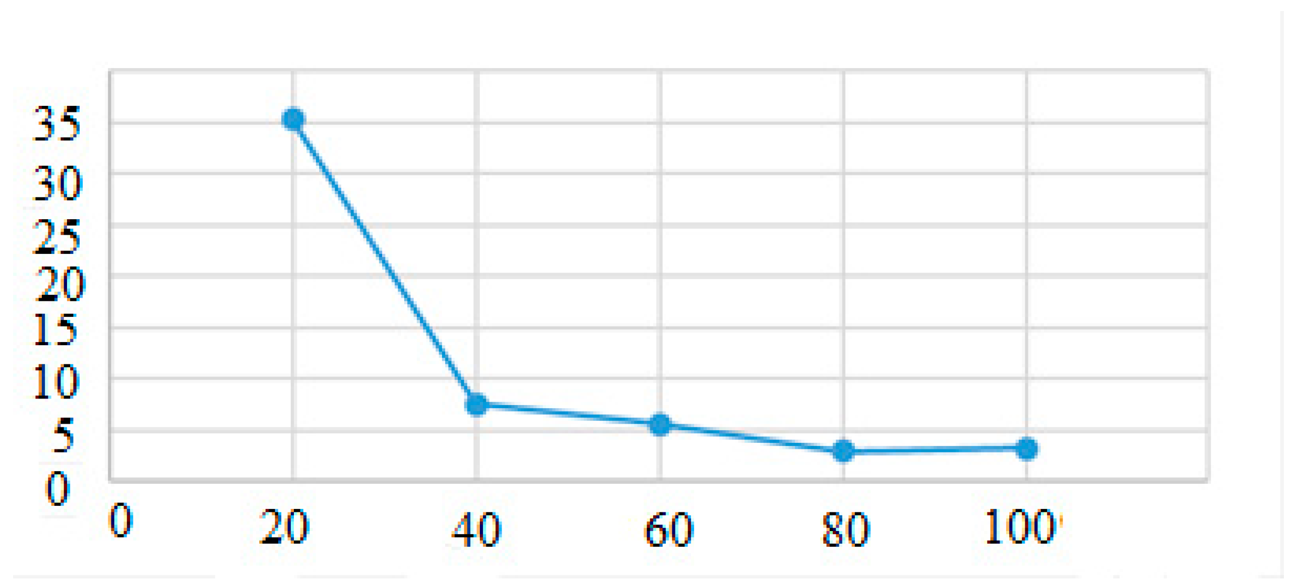
With the same RLDs, we investigated the error number depending the training cycle number. Figure 20 demonstrates the improvements in recognition with an increase in the cycle number. With 100 training cycles, the recognition rate was 98.5%.

In

Table 8. Recognition.

Number of Classes	Recognition Rate (%)
5	100
10	98.57
15	99.04
20	99.28
25	98.85
30	99.04
35	98.77
40	98.57
45	98.41
50	97.71
100	96.85

, we present the recognition statistics for different numbers of classes but with the same number of RLDs. In this case, we used 400 features (RLDs).

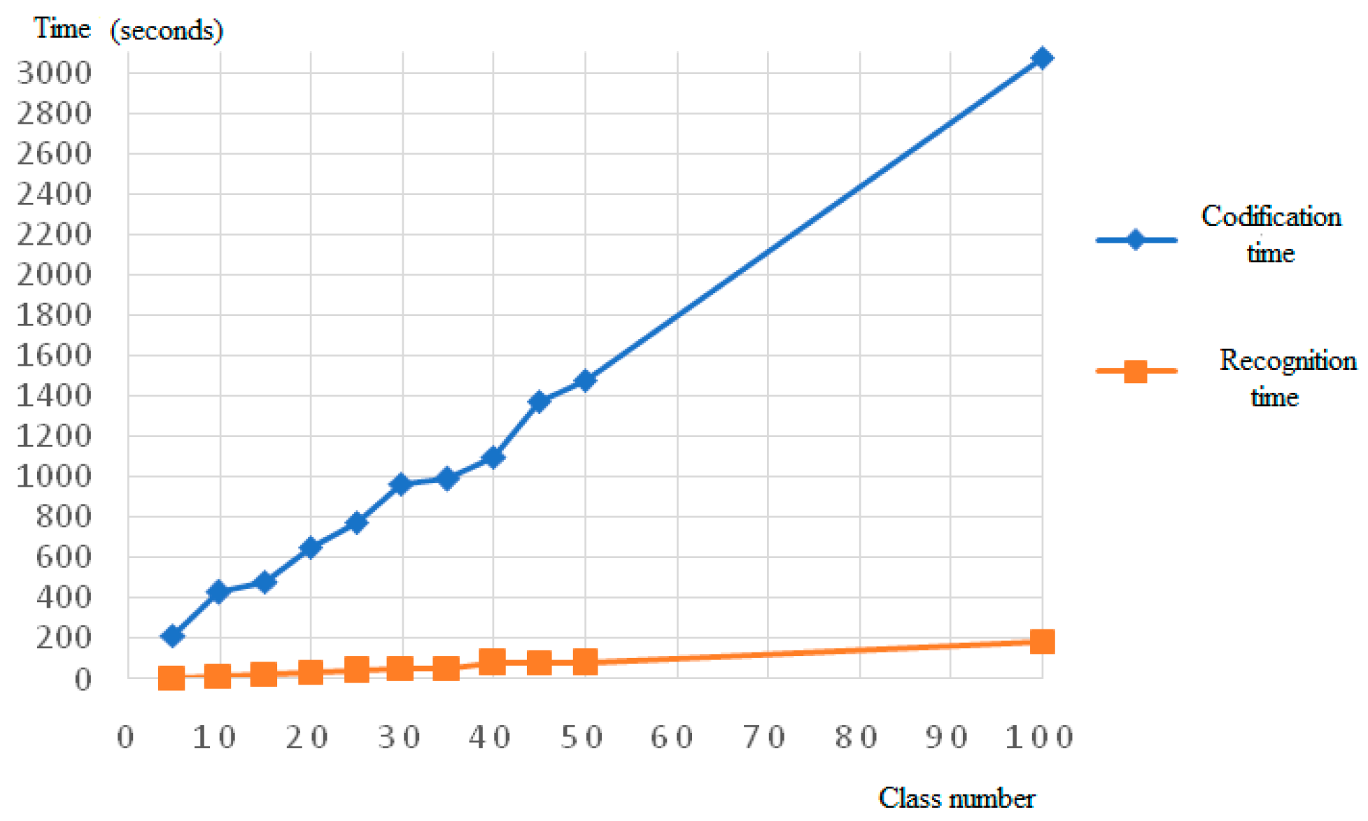
The time of coding and recognition processes for PCNC with RLDs are presented in Figure 21.

The experiments with the PCNC, RLDs and the FEI image dataset yieldedgood results.

In this article, we investigated RLDs and compared their influence on image recognition with LBP algorithms.

5. Conclusions

The PCNC neural classifier is based on the RLD descriptors that are used for feature extraction from the image. We compared our method with the LBP principle often used in facial recognition. The PCNC neural classifier presented good results in facial recognition using the ORL, FRAV3D and FEI image databases. We demonstrated that our system yielded results better than those obtained using other methods, especially LBP. Our RLDs have advantages, because they require less time for calculations, and the number of RLDs is less than that required for LBPs. To obtain these results, we generated additional images for the training set using image distortions. First, the simplest distortions, including image displacements, were investigated. . Sometimes, we obtained twice the decrease in error for the FRAV3D image database. It was done many experiments with RLDs. It was shown that the RLD parameters have an influence on face recognition quality. We showed that RLD is a good alternative to LBPs, and that our model is a good approach for face feature detection using local descriptors. The PCNC with the RLDs demonstrated the best recognition rate, i.e., 97.49%, in comparison with 90.49% for LBPs for the ORL image database. For the FEI image database, we obtained the best recognition rate, i.e., 93.57%, in comparison with 66.74% for the LBPs. For FRAV3D, we improved the recognition rate by decreasing by approximately twice the number of errors using the RLDs and rotation of original images..