The Optimal Transportation Option in an Underground Hard Coal Mine: A Multi-Criteria Cost Analysis

Abstract

The issue of transport in underground hard coal mines is very rarely described in the literature. The financial aspects of this issue are even less often analyzed. Publications in this area focus on technical issues and the safety of mining crews. More attention is paid to transport in open-pit mines. The above premises and practical needs imply the need to conduct economic analyses of transport systems in underground hard coal mines. This paper is a scientific communication, which presents the concept of a multi-criteria cost analysis as a tool to support the selection of the optimal transportation option in an underground hard coal mine. Considerations in this area have not been carried out in the relevant literature, and the problem of selecting a transportation option is a complex and necessary issue in the practice of underground mines with extensive mine workings. The methodology presented includes five cost criteria (costs of carrying out the transportation task; route expansion costs; rolling stock maintenance costs; depreciation costs; and additional personnel costs). The simultaneous application of criteria relating to utility properties in addition to cost criteria makes it possible to adopt a specific technical and organizational model of the transportation system based on the indication of the optimal solution, resulting from the mathematical construction of functions of objectives relating to utility and cost. The optimal variant of the designed system and configuration of the material transportation system in underground workings takes into consideration the following: (1) seven utility criteria (KU1—transportation task completion time; KU2—compatibility of transportation systems; KU3—continuous connectivity; KU4—co-use with other transportation tasks; KU5—safety; KU6—inconvenience; KU7—operation under overplanning conditions) and (2) five cost criteria (KK1—costs of implementing the transportation task; KK2—costs of route expansion; KK3—rolling stock maintenance costs; KK4—depreciation costs; KK5—additional personnel costs). Based on the aforementioned criteria, two objective functions are built for each option: utility and cost. They present divergent goals; therefore, they are non-cooperative functions. Both utility and costs strive for the maximum. In the developed methodology, an ideal point is usually a fictitious solution representing a set of maximum values among all the achievable values in a set of solutions, but it is impossible to achieve this simultaneously based on all the criteria. This point illustrates the maximum utility and lowest cost among the alternatives considered, which is obviously impossible for any of the variants to meet at the same time, although it indicates the possibilities of the technique and the range of costs. For the developed method, a so-called “PND” nadir point is also determined, representing the least-preferred level of achievement of all goals simultaneously, determined from the set of optimal points in the Pareto sense. The originality of the conceptual considerations undertaken stems from: filling the gap in the economic methodology of complex transportation systems evaluation; embedding considerations in the trend concerning complex transportation systems of underground mines; and focusing considerations on the pre-investment phase, making it possible to optimize costs before expenditures are incurred.

1. Introduction

The transportation system in an underground hard coal mine must be adapted to both geological and mining conditions and the mining schedule. In Polish coal mines, the appropriate design of such a system is a very complex task due to the vastness of underground mine workings and the difficult mining conditions (high level of mining hazards and great depth of extraction) [1,2,3].

In addition, currently, in the mines of the Upper Silesian Coal Basin, all means of self-propelled transport are used: track rail with electric and diesel locomotives, suspension railroads, and floor railways. In all mines, transport systems are used (to varying extents) for the regular transport of materials used in the working faces, heavy loads (in particular during reinforcement and decommissioning works), and for the transport of crew [4,5].

In selecting the right design of the transportation system, a multi-criteria analysis can be of assistance, the use of which the authors of this study proposed in the pages of the Resources journal in October 2023 [6] to determine the technical aspects of underground cargo movement.

In addition to technical aspects, optimization of underground transportation costs is equally important, as it affects the ultimate profitability of the extraction process [7,8]. In Polish mines, this is of particular importance due to EU restrictions on the prohibition of subsidizing unprofitable mines from the state budget [9].

Meanwhile, the literature and mining practice lack comprehensive methods to support decision-making regarding the selection of an underground transportation system also based on financial criteria. In the case of complex transportation systems, developing an effective methodology in this regard is not easy, as it does not just boil down to simple cost estimation, instead requiring consideration of many criteria and circumstances. In the future, this issue, due to the depletion of deposits and the need to extract under increasingly difficult conditions, may gain importance beyond the area of the European Union.

Currently, in the context of underground transportation, the literature primarily addresses technical issues related to underground coal gasification, including An et al. (2022) [10], Zagorščak et al. (2019) [11], and Soukup et al. (2014) [12]. Transportation issues are also examined in the context of ensuring the safety of mining crews, including in the studies by Tu et al. 2023 [13], Li et al. (2022) [14], Fabiano et al. (2014) [15], and Thakur (2019) [16]. This trend also includes advanced studies on unmanned transportation carried out in the spirit of smart technologies, as demonstrated by Wang et al. (2022) [17]. Transportation also appears as a subject of consideration for individual links of mining production, such as in Yuan et al. 2022 [18], Krauze et al. (2020) [19], and Szewerda et al. (2021) [20].

The strength of the above-mentioned mining transport solutions is certainly the proposal and promotion of modern technologies in an industry considered traditional and in decline. The studies cited are also very detailed and solve specific process problems. Nevertheless, it seems that the solutions described are mainly future technologies. They are experimental, expensive, and very specific, which limits their application. Meanwhile, in modern mining, many difficult issues are not spectacular but urgently require ready-made solutions. One of them is to improve economic efficiency while meeting technological requirements and ensuring occupational safety. In this context, the proposed methodology for cost optimization in transport systems is a valuable contribution to the economics of mining.

The financial aspects of transportation solutions are rarely mentioned in scientific publications, although the mining industry is one of the most capital-intensive. In this strand of considerations, one can most often find publications relating to the rationalization or cost reduction of already existing solutions. Therefore, Zhang et al. (2023) [21] seek to reduce transportation costs in open-pit mines by developing an optimal truck driving style. Their research shows that standardizing driver behavior can result in a 5% reduction in transportation costs, which, given the 50% share of these costs in total production costs, is important for efficiency levels. The cost intensity of transportation in mines is also confirmed by a study by Teplická et al. (2021) [22].

On the other hand, Fang and Peng (2023) [23] propose the use of autonomous trucks in open-pit mines, which, according to the results of their study, will enable better transportation planning and thus help reduce the cost and time consumption of mining work.

The cost intensity of transportation in open-pit mines is also pointed out by Ren et al. (2023) [24]. To reduce transportation costs, the authors propose scheduling train timetables. The solution they have developed is fully automated and works in real time, improving system throughput and mining productivity.

The proposals described above apply only to open-pit mines. Transport management in underground mines practically does not appear at all in contemporary research and analyses. However, this does not mean that it is a secondary, resolved, or unimportant issue. Due to the depletion of natural raw materials, mining conditions are systematically deteriorating. This increases costs and reduces the profitability of mining production. In this context, all attempts to improve mining efficiency are valuable scientifically and practically.

The importance of economic aspects of mining increases in difficult mining and geological conditions, as emphasized in the analysis by Krysa et al. (2021) [25]. The authors were concerned with optimizing the profitability of mining a low-grade limestone deposit in an open-pit mine. The results of their simulations show that keeping the operating environment in a good state of repair positively affects machine cycle times, the required total transportation task completion time, and operating costs.

Regarding underground mines, Halilović et al. (2023) [26] developed a model to determine the optimal number of ore passes, the optimal location of ore passes, and the optimal dynamic ore transportation plan. The authors treated production and investment costs as determinants of optimization decisions. They used fuzzy set theory to build the model while emphasizing that optimizing transportation systems in underground mines is a difficult and complex task.

The above review shows that there have only been a few attempts to optimize costs in underground mines. They are diagnostic or modeling in nature. They are also often difficult to apply due to the advanced mathematical apparatus requiring additional skills and competencies. The methodology proposed in this article partially eliminates the identified weaknesses. Nevertheless, it is worth adding that due to the holistic approach to optimizing efficiency in underground transport, the research conducted so far is extremely valuable and practical.

Thus, a current review of the literature on the subject shows that researchers are focusing on the technical aspects of mining transportation. On the other hand, the few publications on economic issues focus on open-pit mines and the issue of optimizing the operation of transportation systems already in place. Therefore, there is a lack of publications on the economic and pre-investment basis for selecting transportation systems in underground mines. For these reasons, the purpose of this scientific communication is to present the concept of multi-criteria cost analysis as a tool to support the selection of the optimal transportation option in an underground hard coal mine.

This paper is conceptual in nature, and as a result, the next section presents a proposed methodology for multivariate evaluation of transportation system costs as a basis for selecting the optimal option. The principles of the proposed concept are then demonstrated. The entire paper ends with a summary containing the most relevant conclusions, research limitations, and directions for further research.

The originality of the conceptual considerations undertaken stems from:

• filling the gap in the economic methodology of complex transportation systems evaluation;
• embedding considerations in the trend concerning complex transportation systems of underground mines;
• focusing considerations on the pre-investment phase, making it possible to optimize costs before expenditures are incurred.

2. Materials and Methods

A multi-criteria analysis was used to evaluate individual variants of transport systems in an underground hard coal mine. It is a universal method that allows for taking into account many competing goals and criteria [27,28]. The results obtained using this method are easy to interpret and compare [29].

In underground hard coal mining, investment decisions are made not only based on economic criteria but also on geological and mining criteria related to natural hazards and the safety of mining crews [30,31]. The use of a multi-criteria analysis therefore creates an opportunity to cover most of the quantifiable variables influencing the decision to choose a transport system.

In the literature on the subject, multi-criteria analyses is used to diagnose contemporary mining problems. Most often, these are complex technical issues requiring multi-disciplinary assessments [32,33]. These are also issues related to natural hazards [34]. Nevertheless, according to Baloyi and Meyer (2020) [35], the use of multi-criteria analyses in mining is still not sufficient. Therefore, there is great potential for this method, which we use in this research.

A similar methodological trend is the use of fuzzy logic to assess mining challenges. Jiskani et al. (2022) [36] evaluated strategic development paths for smart and green mining using this methodology. In this way, the authors combined environmental, social, and technological issues. Such analyses fit perfectly into the mining 4.0 trend, which describes mines as modern and environmentally friendly enterprises [37,38,39].

In this article, a multi-criteria analysis is used to synthesize determinants in the field of usability and costs. This synthesis is intended to support the selection of a transport system in a hard coal mine. In the proposed methodology, two objective functions are built for each option: utility (U) and cost (K). They present divergent goals; therefore, they are non-cooperative functions. Both utility and costs strive for the maximum. The optimization of the utility function has been previously described and published [6]. In the case of the utility function, the optimal variant of the designed system and configuration of the material transportation system in underground workings takes into consideration seven utility criteria: KU1—transportation task completion time; KU2—compatibility of transportation systems; KU3—continuous connectivity; KU4—co-use with other transportation tasks; KU5—safety; KU6—inconvenience; and KU7—operation under overplanning conditions.

Now, in this scientific communication, we describe the cost criteria, the synthesis of both functions, and the rules for selecting the optimal variant in terms of usability and costs. The research stages of the presented method are shown in Figure 1.

The designed transportation system, in addition to specific performance characteristics that allow its use in underground mine workings [6], should also allow for the lowest possible costs associated [40] with its development and subsequent operation. In this case, the costs will be expressed in monetary terms as the consumption of fixed assets, intangible assets, materials, fuel, energy, services, employee working time, and the volume of certain expenses that do not reflect consumption but relate to the normal activities of a given economic unit in a certain unit of time [41,42].

It is proposed to identify five criteria differentiating the individual variants of the designed solutions in terms of investment and use. This cost includes:

• KK1: costs of implementing the transportation task;
• KK2: costs of route expansion;
• KK3: rolling stock maintenance costs;
• KK4: depreciation costs;
• KK5: additional personnel costs.

The above cost groups were determined based on detailed analyses of transport costs in several underground hard coal mines in the Upper Silesian Coal Basin. The authors have been dealing with cost issues for several decades. This has been documented in their previous publications, including but not limited to refs. [43,44,45,46,47]. The KK1 and KK2 criteria take into account the investment outlays incurred at the time of implementing the transport solution. The criteria from KK3 to KK5 concern the costs of maintaining the implemented transport system. This approach is holistic because it takes into account both investment expenses and operating costs.

The cost criteria are described in detail later in the methodology. The sum of the weights of each criterion is 100. The distribution of weights depends on the designer, who independently decides the relevance of a criterion. Their sample distribution among the various criteria is shown in

Table 1. Examples of proposed weights for the cost criteria.

Criterion	KK1A	KK1B	KK2	KK3	KK4	KK5
Scoring [K point]	20	10	14	10	16	30

Source: own elaboration.

.

Due to the different distribution and value of costs in transport investment, the authors do not propose fixed weights for individual cost criteria. The weights of individual cost groups will vary depending on the scope of the investment undertaken. They can be determined based on the structure of costs incurred and the total expenditure. This is a simple and objective criterion for selecting criteria weights. The weights can also be adopted based on the average cost structure for previous transport investments based on cost records. This approach allows us to avoid a situation in which costs of less importance (lower share in total costs) have the same impact on the economic assessment of the investment as costs with a significant share in the total cost structure. The costs structure and weights allow us to take into account the “importance of costs,” i.e., their impact on the final amount of investment costs.

In the proposed methodology, expenditures and costs are taken into account at a given moment in time while maintaining a conservative valuation and the geological and mining conditions planned and identified for a given deposit. Of course, in underground mining, every decision carries a high risk due to the unpredictability of natural mining circumstances. Nevertheless, currently, decisions about the choice of a transport system are made intuitively, based on previous experience. Therefore, the proposed method—although imperfect—creates an opportunity for a comprehensive consideration of mining and economic conditions. This is its advantage over the existing pragmatics.

Individual costs are considered to be incurred over the entire period of operation of a given variant of the transportation system (useful life):

$${\mathrm{w}}_{\mathrm{k}}=\sum _{\mathrm{j}=1}^{{\mathrm{n}}_{\mathrm{k}}}{\mathrm{w}}_{\mathrm{k}\mathrm{j}}$$

(1)

where:

• w_k—total cost criterion scoring (100 points),
• n_k—number of cost criteria (pcs)
• w_ki—scoring in the cost criterion “j” (K point).

The number of points is calculated similarly to the utility criteria [6]; the best value of the parameter, i.e., the lowest costs, receives the highest score, and the highest costs receive the lowest score (in these criteria there are only destimulants). However, the method of scoring the variants between the highest and lowest ratings is different; a logarithmic relationship has been used [48]. This better reflects the impact of the implementation of the various options on the magnitude of costs. In the range close to the maximum magnitude, each successive increase “means more,” and conversely, in the range close to the minimum value, the decrease in the magnitude of costs is less significant [49,50]:

$${\mathrm{p}}_{\mathrm{k}\mathrm{i}\mathrm{j}}=\frac{\ln \left[1+({\mathrm{k}}_{\mathrm{m}\mathrm{a}\mathrm{x}}-{\mathrm{k}}_{\mathrm{i}})\right]}{\ln \left[1+({\mathrm{k}}_{\mathrm{m}\mathrm{a}\mathrm{x}}-{\mathrm{k}}_{\mathrm{m}\mathrm{i}\mathrm{n}})\right]}\times {\mathrm{w}}_{\mathrm{k}\mathrm{j}}$$

(2)

where:

• p_kij—scoring of criterion “i” of variant “j” (K point),
• k_max—maximum cost, kmax = max (k₁, …, k_i, …, k_n) (PLN),
• k_min—minimum cost, kmin = min (k₁, …, k_i, …, k_n) (PLN),
• k_i—cost of the variant “i” (PLN),
• w_kj—scoring of the cost criterion “j” (K point).

In the summary of the introduction to the proposed methodology, it is also worth mentioning the disadvantages of a multi-criteria analysis. One of them is the subjectivity of choosing weights for individual criteria. This method also does not take into account the qualitative conditions of the analyzed phenomena. Nevertheless, it is holistic, clear, and easy to use in practice. For these reasons, the authors found it beneficial and possible to use in the assessment of underground transport systems. A detailed description of the individual cost criteria (the second area of the proposed methodology) is presented in the following subsections. Then, the rules for selecting the optimal variant are described along with a demonstration case.

2.1. KK1 Criterion—Costs of Implementing the Transportation Task

This criterion describes the costs depending on the number of transportation tasks completed. The assumption of all variants refers to the same location of the receiving and sending point and the same amount of cargo. It is crucial to determine the reference number of transportation units, since in different solutions, it is possible that the same number of units can be moved in one or more cycles. The costs of carrying out a transportation task consist of fuel or electricity, labor, depreciation and consumables, maintenance, and repair [51]:

K_zt = K_p + K_r + K_a + K_e

(3)

where:

• K_zt—costs of implementing the transportation task (PLN),
• K_p—cost of fuel or electricity (PLN),
• K_r—labor cost (PLN),
• K_a—depreciation cost of the means of transportation (PLN),
• K_e—cost of consumables, maintenance and repair (PLN).

Manufacturers of diesel-powered tractors and locomotives specify fuel consumption in unit values, i.e., the mass of fuel consumed by an engine of a given horsepower running for a given period (g/kWh). The engine power of the equipment is given in its data sheet. It is important to determine the operating time of the internal combustion engine and the level of use of its power. Due to the use of hoists powered by hydraulic oil from a diesel–hydrostatic unit, the operating time of the diesel engine for suspension railroads also includes the loading and unloading phases. The level of power utilization during the operating cycle depends on the slope of the route, the weight of the load, and the number of hydraulic-powered crane devices used. Based on the results of a comparison of the actual fuel consumption against the designated one for maximum power made at one of the mines, it was found that the level of power utilization was in the range of 70–90%.

In the case of electric-powered suspension railroad tractors, it can be assumed that the level of power utilization is in the range of 80–90%.

The cost of fuel for internal combustion-powered means of transportation is calculated as follows:

$${\mathrm{K}}_{\mathrm{p}}=\frac{{\mathrm{z}}_{\mathrm{p}\mathrm{P}}\times {{\mathrm{p}}_{\mathrm{s}\mathrm{s}}\times \mathrm{P}}_{\mathrm{P}}\times ({\mathrm{t}}_{\mathrm{z}\mathrm{t}\mathrm{p}}-{\mathrm{t}}_{\mathrm{o}\mathrm{t}})\times {\mathrm{k}}_{\mathrm{o}\mathrm{n}}}{60\times {\mathrm{\delta }}_{\mathrm{p}}}$$

(4)

The cost of electricity for electrically powered means of transportation is calculated as follows:

$${\mathrm{K}}_{\mathrm{e}}=\frac{{\mathrm{P}}_{\mathrm{P}}\times {\mathrm{p}}_{\mathrm{s}\mathrm{e}}\times ({\mathrm{t}}_{\mathrm{z}\mathrm{t}\mathrm{p}}-{\mathrm{t}}_{\mathrm{o}\mathrm{t}})\times {\mathrm{k}}_{\mathrm{p}\mathrm{e}}}{60}$$

(5)

After taking into account the labor costs:

$${\mathrm{K}}_{\mathrm{z}\mathrm{t}\mathrm{s}}=\left({\mathrm{t}}_{\mathrm{z}\mathrm{t}\mathrm{p}}-{\mathrm{t}}_{\mathrm{o}\mathrm{t}}\right)\times \left(\frac{{\mathrm{z}}_{\mathrm{p}\mathrm{P}}\times {{\mathrm{p}}_{\mathrm{s}\mathrm{s}}\times \mathrm{P}}_{\mathrm{P}}\times {\mathrm{k}}_{\mathrm{o}\mathrm{n}}}{60\times {\mathrm{\delta }}_{\mathrm{p}}}\right)+\left(\frac{{\mathrm{r}}_{\mathrm{d}\mathrm{o}}+{\mathrm{r}}_{\mathrm{d}\mathrm{m}}}{{\mathrm{z}}_{\mathrm{z}\mathrm{m}\mathrm{i}}}\right)$$

(6)

$${\mathrm{K}}_{\mathrm{z}\mathrm{t}\mathrm{e}}=\left({\mathrm{t}}_{\mathrm{z}\mathrm{t}\mathrm{p}}-{\mathrm{t}}_{\mathrm{o}\mathrm{t}}\right)\times \left(\frac{{\mathrm{P}}_{\mathrm{p}}\times {\mathrm{p}}_{\mathrm{s}\mathrm{e}}\times {\mathrm{k}}_{\mathrm{p}\mathrm{e}}}{60}\right)+\left(\frac{{\mathrm{r}}_{\mathrm{d}\mathrm{o}}+{\mathrm{r}}_{\mathrm{d}\mathrm{m}}}{{\mathrm{z}}_{\mathrm{z}\mathrm{m}\mathrm{i}}}\right)$$

(7)

where:

• K_p—fuel cost (PLN),
• K_e—electricity cost (PLN),
• K_zts(e)—cost of carrying out the transportation task using internal combustion (electric) means of transportation (PLN),
• z_pP—unit fuel consumption of the tractor (g/kWh),
• P_p—engine power (kW),
• p_ss—motor power utilization factor (0.7–0.9),
• p_se—electric motor power utilization factor (0.8–0.9),
• k_on—unit cost of fuel (PLN/dm³),
• k_pe—unit cost of electricity (PLN/kWh),
• δ_p—fuel density (kg/m³),
• r_do—value of an operator’s working day (PLN),
• r_dm—value of a shunter’s working day (PLN),
• t_ot—duration of maintenance (min),
• t_ztp—duration of transport to an average distant point (min),
• z_zmi—number of transport tasks possible during a shift.

In the case of tractors of the floor railways and locomotives of the underground railroad, the engine does not run during loading and unloading, and the partial times corresponding to these activities are negligible (in locomotives of the underground railroad, the shunting time is generally extended).

For transportation with transloading phase(s), it is necessary to calculate the sum of the transportation costs within each transportation system:

$${\mathrm{K}}_{\mathrm{z}\mathrm{t}}=\sum _{\mathrm{i}=1}^{\mathrm{n}}{\mathrm{k}}_{\mathrm{z}\mathrm{t}\mathrm{i}}$$

(8)

In this criterion, the highest scoring value is the lowest cost of implementing the transportation task. This variant receives the maximum number of points, and the variant with the highest costs receives zero points. The remaining variants receive a score according to the logarithmic relationship given in Formula (2), which in this case are as follows:

• k_max = k_{zt max}—highest cost of implementing the transportation task (PLN),
• k_min = k_{zt min}—lowest cost of implementing the transportation task (PLN),
• k_i = k_zti—cost of implementing the transportation task in the variant “i” (PLN),
• w_kj = w_kk1—weight, the maximum number of points in criterion KK1 (K point).

A summary of the KK1 criterion score is presented in

Table 2. Criterion KK1—costs of carrying out transportation tasks.

Variants	Total Cost (PLN)	Weight: wkk1 (K Point)
W1	Kztsz 1	pkk1 1
…	…	…
Wi	Kztsz i	pkk1 i
…	…	…
Wn	Kztsz n	pkk1 n

Source: own elaboration.

.

2.2. Criterion KK2—Costs of Route Expansion

This criterion describes the costs of further track expansion in the event of changes in the transport routes. These are variable costs. The assumptions of all variants are as follows: the route leads in a new pit, the required traffic gage is provided, and the comparative section is straight.

The cost of extending the rail track of the transportation system in underground pits consists of the cost of the purchase of components and elements of a particular type of transportation system, their delivery to the place of installation, labor, reconstruction of pits in terms of obtaining the required gage, reinforcement of the lining, etc.:

$${\mathrm{K}}_{\mathrm{rt}}={\mathrm{K}}_{\mathrm{rcz}}+{\mathrm{K}}_{\mathrm{rzt}}+{\mathrm{K}}_{\mathrm{rr}}+{\mathrm{K}}_{\mathrm{rp}}+{\mathrm{K}}_{\mathrm{mech}}$$

(9)

where:

• K_rt—cost of route expansion (PLN),
• K_rcz—total cost of track elements (PLN),
• K_rzt—cost of transporting track elements (PLN),
• K_rr—labor cost (PLN),
• K_rp—cost of pit reconstruction (PLN),
• K_mech—cost of using mechanization equipment for track construction (PLN).

The basic sections of the various tracks vary in length. Examples of their size, as used in mines, are shown in

Table 3. Lengths of basic route sections of different types of transport systems used in mines.

Transportation System Type	Lengths of Basic Route Sections
Underground railroad	5.0; 6.0 m
Floor railways	2.0–3.0 m
Suspension railroad	Rail lengths: 1.6 m; 2.0 m; 2.4 m; 2.5 m; 3.0 m. Lateral stabilization—every 20–30 m

Source: own elaboration.

.

Therefore, it is necessary to adopt a specific length of the so-called “elementary track section” that is identical in terms of length in all variants—this will be a section equal to 1 m. However, due to the different number of fastening and fixing elements, depending on the type of transportation system as well as the length of the rail, it is necessary to first calculate the cost of materials of the elementary track section, specific to the adopted solution:

$${\mathrm{k}}_{\mathrm{t}\mathrm{e}\mathrm{m}\mathrm{i}}=\frac{{\mathrm{k}}_{\mathrm{p}\mathrm{i}}}{{\mathrm{l}}_{\mathrm{p}\mathrm{i}}}$$

(10)

where:

• k_temi—cost of materials of the elementary track section type “i” (PLN/m),
• k_pi—cost of materials of the basic track section of type “i” (PLN),
• l_pi—length of the basic track section of type “i” (m).

The labor costs of building an elementary section of track k_teri are calculated as follows:

$${\mathrm{k}}_{\mathrm{t}\mathrm{e}\mathrm{r}\mathrm{i}}=\frac{{\mathrm{k}}_{\mathrm{c}\mathrm{s}}\times {\mathrm{n}}_{\mathrm{c}\mathrm{s}\mathrm{i}}}{{\mathrm{p}}_{\mathrm{t}\mathrm{i}}}$$

(11)

where:

• k_cs—labor cost per day of a track carpenter (PLN),
• n_csi—occupancy of a brigade of track carpenters to build track type “i” (person),
• p_ti—length of track section of type “i” built in one shift by a brigade of track carpenters (m).

The costs of building the elementary section k_tei are calculated as follows:

$${\mathrm{k}}_{\mathrm{t}\mathrm{e}\mathrm{i}}={\mathrm{k}}_{\mathrm{t}\mathrm{e}\mathrm{m}\mathrm{i}}+{\mathrm{k}}_{\mathrm{t}\mathrm{e}\mathrm{r}\mathrm{i}}$$

(12)

In addition to the development of straight sections of the route, it may be necessary to develop a certain number of curved rails (route turns) or turnouts. Their costs consist of the cost of materials used k_mł(r) and labor costs k_rł(r):

$${\mathrm{k}}_{\mathrm{r}ł\left(\mathrm{r}\right) \mathrm{e}}={\mathrm{k}}_{\mathrm{m}ł\left(\mathrm{r}\right)}+{\mathrm{k}}_{\mathrm{r}ł\left(\mathrm{r}\right)}={\mathrm{k}}_{\mathrm{m}ł\left(\mathrm{r}\right)}+\frac{{\mathrm{k}}_{\mathrm{c}\mathrm{s}}\times {\mathrm{n}}_{\mathrm{c}\mathrm{s}}}{{\mathrm{n}}_{\mathrm{ł}\left(\mathrm{r}\right)}}$$

(13)

where:

• k_cs—labor cost per day of a track carpenter (PLN),
• n_cs—occupancy of a brigade of track carpenters to build curves of the route or turnouts (person),
• n_ł(r)—number of curves (turnouts) built during one shift by a brigade of track carpenters (pcs).

Depending on the type of transportation system, the basic fasteners and fixing elements are:

• mine underground railroad track—bolts and nuts of various sizes, washers, spacers, lugs,
• suspension railroad track—slings, traverses, chains, brackets, stays, bolts,
• floor railways track—bolts and nuts of various sizes, anchors, and railroad loads.

In the case of variants consisting of different types of transportation systems, the elementary (mixed) section for comparison with other variants is determined as a weighted average, where the weights correspond proportionally to the share of sections of a given type of system in the total transport routes. Then, usually only one type of transportation system covers the face-adjacent zones, and it is usually the one that will be expanded.

Based on the cost of an elementary route section, the cost of extending a transportation route can be determined, including the cost of curves and turnouts:

$${\mathrm{K}}_{\mathrm{r}\mathrm{p}}=\sum _{\mathrm{i}=1}^{{\mathrm{m}}_{\mathrm{u}\mathrm{k}}}{\alpha }_{ri} \left({\mathrm{k}}_{\mathrm{t}\mathrm{e}\mathrm{i}}\times {\mathrm{l}}_{\mathrm{d}\mathrm{i}}+{{\mathrm{k}}_{\mathrm{r}\mathrm{i}}\times \mathrm{n}}_{\mathrm{r}\mathrm{r}\mathrm{i}}+{{\mathrm{k}}_{\mathrm{ł}\mathrm{i}}\times \mathrm{n}}_{\mathrm{ł}\mathrm{i}}\right)$$

(14)

where:

• K_rp—cost of transportation route expansion (PLN),
• m_uk—number of types of transportation systems (pcs),
• α_ri—the probability of expansion of transport system type “i”
• (α_r1 + … + α_rn = 1),
• k_tei—cost of an elementary section of track type “i” (PLN/m),
• l_di—length of track section of type “i” (m),
• k_ri—cost of building a turnout of track type “i” (PLN/pc),
• n_rri—number of turnouts in the transportation system of type “i” (pcs),
• k_łi—cost of building a curve of track type “i” (PLN/pc),
• n_łi—number of curves in the transportation system of type “i” (pcs).

In the criterion, the highest-scoring value is the lowest cost K_rp—this variant receives the maximum number of points, and the variant with the highest costs receives zero points. The remaining variants receive a score according to the logarithmic relationship given in Formula (2), which in this case is:

• k_max = k_rpmax—highest route expansion costs (PLN),
• k_min = k_rpmin—lowest route expansion costs (PLN),
• k_i = k_rpi—cost of route expansion in the variant “i” (PLN),
• w_kj = w_kk2—weight, the maximum number of points in criterion KK2 (K point).

A summary of the KK2 criterion score is presented in

Table 4. Criterion KK2—costs of route expansion.

Variants	Expansion Cost (PLN)	Weight: wkk3 (K Point)
W1	Krp 1	pkk2 1
…	…	…
Wi	Krp i	pkk2 i
….	…	…
Wn	Krp n	pkk2 n

Source: own elaboration.

.

2.3. Criterion KK3—Rolling Stock Maintenance Costs

This criterion describes the cost of consumables, maintenance, and repairs. At the stage of designing transportation systems and equipment, it is often not possible to determine the exact type of tractor or locomotive (for example, it will be known after the award of the tender). Therefore, it is necessary to rely on the accepted estimated costs of the transportation means to date. If the selected tractor or locomotive is different from those used before, for example, in terms of tractive force (especially in the case of suspension railroads), the cost of use will also be different—for example, because of an engine with a different horsepower and capacity or a different number of hydraulic motors.

It may happen that to guarantee smooth operation in over-plan or emergency states, some variant envisages the use of more transport sets, not all of which will be used in the base state. For this reason, a correction factor should be introduced for the level of use of sets “b_u”:

$${\mathrm{b}}_{\mathrm{u}}=\frac{{\mathrm{n}}_{\mathrm{d}\mathrm{b}}}{{\mathrm{n}}_{\mathrm{d}}\times {\mathrm{g}}_{\mathrm{t}}}$$

(15)

where:

• n_db—designated number of rolling stock to the baseline (pcs),
• n_d—adjusted number of rolling stock (pcs),
• g_t—technical readiness factor of rolling stock type “i”.

Rolling stock maintenance costs consist of maintenance costs (materials and consumables, minor repairs) and labor and maintenance costs [52]:

$${\mathrm{K}}_{\mathrm{u}}=({\mathrm{k}}_{\mathrm{ot}}+{\mathrm{k}}_{\mathrm{np}})+({\mathrm{k}}_{\mathrm{rot}}+{\mathrm{k}}_{\mathrm{rnp}})$$

(16)

where:

• K_u—maintenance costs (PLN),
• k_ot—cost of materials and consumables (PLN),
• k_np—the cost of spare parts replaced during repairs (PLN),
• k_rot—labor cost—maintenance (PLN),
• k_rnp—labor cost—repairs and overhauls (PLN).

Maintenance labor costs:

$${\mathrm{k}}_{\mathrm{otm}}=\frac{{\mathrm{k}}_{\mathrm{e}\mathrm{m}}}{12}\times ({\mathrm{n}}_{\mathrm{wp}}+{\mathrm{n}}_{\mathrm{zt}})$$

(17)

where:

• k_otm—monthly cost of maintenance (workshop) of rolling stock “i” (PLN),
• k_em—annual labor cost of an employee in the position of a mechanic of tractors/locomotives of rolling stock “i” (PLN),
• n_wp—workshop occupancy (person),
• n_zt—occupancy of non-workshop shifts (person).

Taking into account the proposed coefficients, the cost of parts and consumables can be compared to the cost of a reference standard tractor used to date:

$${\mathrm{k}}_{\mathrm{umi}}={\mathrm{m}}_{\mathrm{t}} \times {\mathrm{b}}_{\mathrm{ui}} \times {\mathrm{k}}_{\mathrm{s}}$$

(18)

where:

• k_umi—monthly cost of materials for tractor type “i” (PLN/month),
• b_ui—utilization factor of rolling stock of type “i”,
• k_s—monthly cost of using a standard tractor under standard conditions (PLN),
• m_t—“strain” factor of a type “i” tractor:

$${\mathrm{m}}_{\mathrm{t}}=\frac{{\mathrm{m}}_{\mathrm{t}\mathrm{r}\mathrm{z}\mathrm{i}}}{{\mathrm{m}}_{\mathrm{t}\mathrm{s}}}$$

(19)

where:

• m_trzi—the actual number of motoring hours per month (mth),
• m_ts—the standard number of motoring hours per month (mth).

If different modes of transportation are used (e.g., due to tractive force or means of propulsion), the costs of using each type of vehicle should be added up:

$${\mathrm{K}}_{\mathrm{u}}={\sum }_{\mathrm{i}=1}^{\mathrm{n}}{\mathrm{n}}_{\mathrm{c}\mathrm{i}}\times {\mathrm{k}}_{\mathrm{u}\mathrm{m}\mathrm{i}}+{\mathrm{k}}_{\mathrm{o}\mathrm{t}\mathrm{m}\mathrm{i}}$$

(20)

where:

• n_ci—number of tractors of type “i” (pcs).

In the criterion, the highest scoring value is the lowest rolling stock maintenance costs. This variant receives the maximum number of points, and the variant with the highest costs receives zero points. The remaining variants receive a score according to the logarithmic relationship given in Formula (2), which in this case is:

• k_max = k_umax—highest cost of use (PLN),
• k_min = k_umin—lowest cost of use (PLN),
• k_i = k_ui—cost of use in the variant “i” (PLN),
• w_kj = w_kk3—weight, the maximum number of points in criterion KK3 (K point).

The summary of the KK3 criterion score is presented in

Table 5. Criterion KK3—rolling stock maintenance costs.

Variants	Cost of Use (PLN)	Weight: wkk3 (K Point)
W1	Ku 1	Pkk3 1
…	…	…
Wi	Ku i	Pkk3 i
…	…	…
Wn	Ku n	Pkk3 n

Source: own elaboration.

.

2.4. Criterion KK4—Depreciation Costs

Depreciation is made as a systematic, scheduled distribution of the initial value of a fixed asset over a fixed period, known as the depreciation period. Fixed assets include, among others, transportation equipment [53]. The basic fixed assets used in underground transportation systems are the following: rolling stock, tractors and locomotives, underground railroad cars, platforms of floor railways and transport assemblies of suspension railroads, mining containers, tracks, and infrastructure and traffic control and protection systems including communications. The investment life cycle is the same as the investment process. This is analogous to the product life cycle; however, the investment life cycle has its specificity—it is often referred to as the investment cycle or investment process. It generally consists of three main phases: pre-investment, investment (implementation), and operation, each of which contains several stages [54]. The depreciation period need not be equal to the useful life. The calculation of this criterion uses the depreciation period: the components of a given transportation subsystem that, at the end of their useful life, are still operable equipment and machinery that can be utilized in another location. In the case of track sections that are heavily used, especially in the case of suspension railroads, the depreciation period will be relatively short. This is due to the wear and tear of the rails. If the depreciation period of the entire transportation subsystem will be longer, the replaced track rails should also be taken into account. This is an example of “asset renewal” with depreciation calculated on a straight-line basis—the value of fixed assets will be increased by their modernization [34]. Since the repair costs of tractors and locomotives were included in the use criterion, they will no longer be included in this criterion.

The monthly depreciation costs will be calculated according to the following formula:

$${\mathrm{K}}_{\mathrm{a}}=\frac{{\mathrm{K}}_{\mathrm{c}\mathrm{l}}}{{\mathrm{T}}_{\mathrm{a}\mathrm{c}\mathrm{l}}}+\frac{{\mathrm{K}}_{\mathrm{c}\mathrm{w}}}{{\mathrm{T}}_{\mathrm{a}\mathrm{c}\mathrm{w}}}+\frac{{\mathrm{K}}_{\mathrm{c}\mathrm{t}}}{{\mathrm{T}}_{\mathrm{a}\mathrm{t}}}+\frac{{\mathrm{K}}_{\mathrm{c}\mathrm{d}}}{{\mathrm{T}}_{\mathrm{a}\mathrm{c}\mathrm{d}}}+\frac{{\mathrm{K}}_{\mathrm{i}\mathrm{n}}}{{\mathrm{T}}_{\mathrm{a}\mathrm{i}\mathrm{n}}}+\frac{{\mathrm{K}}_{\mathrm{w}}}{{\mathrm{T}}_{\mathrm{a}\mathrm{w}}}$$

(21)

where:

• K_a—depreciation cost (PLN),
• K_cl—cost of purchasing transport sets, locomotives and carts, (PLN),
• K_cw—cost of purchasing carts, platforms, transport sets (PLN),
• K_ct—cost of purchasing the tracks with infrastructure (PLN),
• K_cd—cost of purchasing traffic control and protection systems (PLN),
• K_in—cost of purchasing equipment for construction and maintenance of the tracks (PLN),
• K_w—cost of pit excavation (PLN),
• T_ai—depreciation period (month).

In the criterion, the highest-rated value is the lowest value of depreciation write-offs. This variant receives the maximum number of points, and the variant with the highest value receives zero points. The remaining variants receive a score according to the logarithmic relationship given in Formula (2), which in this case is:

• k_max = k_amax—highest value of depreciation write-offs (PLN),
• k_min = k_amin—lowest value of depreciation write-offs (PLN),
• k_i = k_ai—value of depreciation write-offs in the variant “i” (PLN),
• w_kj = w_kk4—weight, the maximum number of points in criterion KK4 (K point).

A summary of the KK4 criterion score is presented in

Table 6. Criterion KK4—depreciation costs.

Variants	Depreciation Cost (PLN)	Weight: wkk4 [K Point]
W1	Ka 1	Pkk4 1
…	…	…
Wi	Ka i	Pkk4 i
…	…	…
Wn	Ka n	Pkk4 n

Source: own elaboration.

.

2.5. Criterion KK5—Additional Personnel Costs

This criterion takes into account additional occupancy—the number of people who may need to be additionally employed in the considered variant regarding the existing volume of employment in transportation services:

$${\mathrm{K}}_{\mathrm{o}\mathrm{r}}={\sum }_{\mathrm{i}=1}^{{\mathrm{m}}_{\mathrm{o}}}{\mathrm{n}}_{\mathrm{o}\mathrm{i}}\times {\mathrm{k}}_{\mathrm{o}\mathrm{i}}$$

(22)

where:

• K_or—annual cost of hiring additional employees (PLN),
• k_oi—annual cost per employee for position “i” (PLN),
• n_oi—number of persons employed in position “i” (person),
• m_o—number of additional positions (pcs).

Additional personnel costs for each option over the considered useful life of the designed transportation system are calculated as follows:

$${\mathrm{K}}_{\mathrm{o}\mathrm{m}}=\frac{{\mathrm{T}}_{\mathrm{u}}}{12}{\sum }_{\mathrm{i}=1}^{{\mathrm{m}}_{\mathrm{o}}}{\mathrm{n}}_{\mathrm{o}\mathrm{i}}\times {\mathrm{k}}_{\mathrm{o}\mathrm{i}}$$

(23)

where:

• T_u—useful life of the designed transportation system (months).

In the criterion, the highest-scoring value is the lowest cost of additionally employed workers. This variant receives the maximum number of points, and the variant with the highest costs receives zero points. The remaining variants receive a score according to the logarithmic relationship given in Formula (2), which in this case is:

• k_max = k_omax—highest cost of additional employment of employees (PLN),
• k_min = k_omin—lowest cost of additional employment of employees (PLN),
• k_i = k_i—cost of additional employment of employees in the variant “i” (PLN),
• w_kj = w_kk5—weight, the maximum number of points in criterion KK5 (K point).

A summary of the KK5 criterion score is presented in

Table 7. Criterion KK5—additional personnel costs.

Variants	Cost of Additional Employment (PLN)	Weight: wkk5 (K Point)
W1	Ko 1	Pkk5 1
…	…	…
Wi	Ko i	Pkk5 i
….	…	…
Wn	Ko n	Pkk5 n

Source: own elaboration.

.

3. Results

To demonstrate how to determine the optimal variant of the designed system and configure the material transportation system in underground workings, the following will be used:

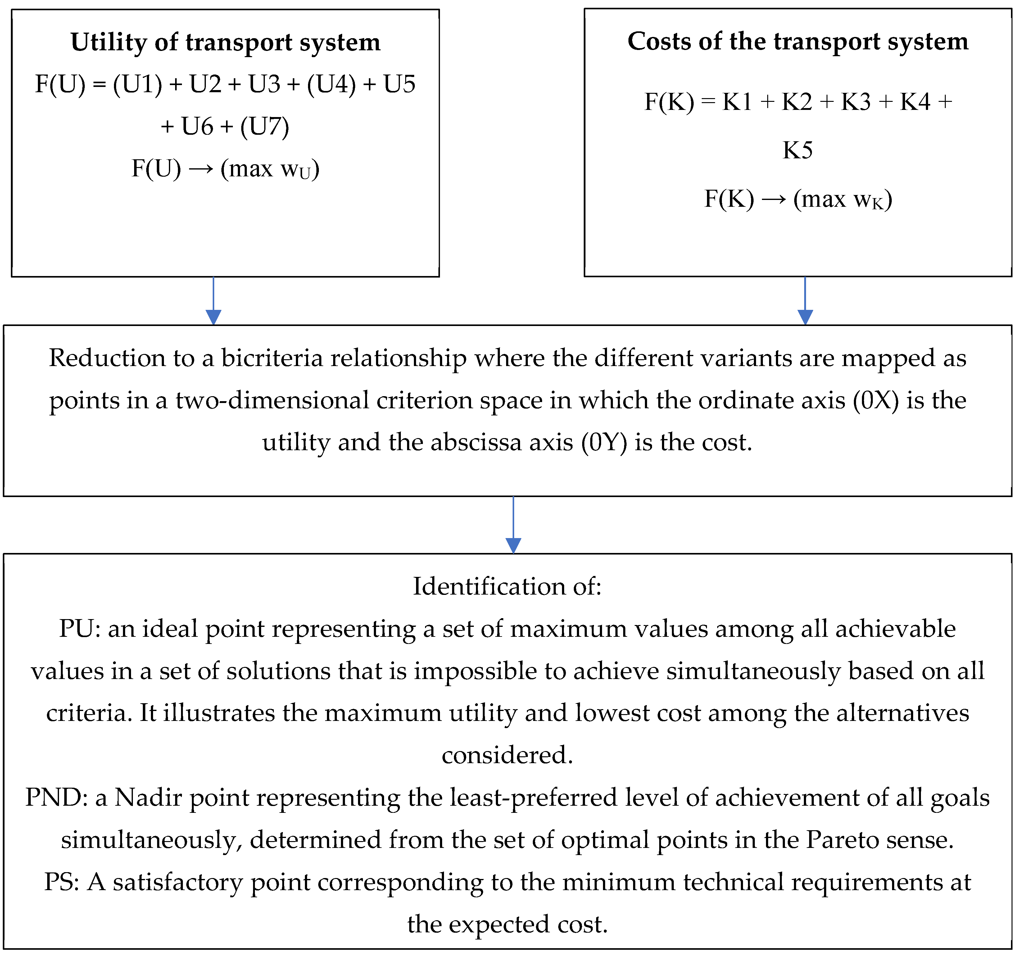
• seven utility criteria (as defined in the article Selection of the optimal design option for transportation systems. Part I—establishment and application of utility criteria [6]) (these criteria include: KU1—transportation task completion time; KU2—compatibility of transportation systems; KU3—continuous connectivity; KU4—co-use with other transportation tasks; KU5—safety; KU6—inconvenience; KU7—operation under overplanning conditions);
• five cost criteria.

Based on the aforementioned criteria, two objective functions are built for each option: utility and cost. They present divergent goals; therefore, they are non-cooperative functions.

Concerning the established utility criteria, the utility function will have the following form:

$$\begin{gathered} \mathrm{F}\left(\mathrm{U}\right)=(\mathrm{U}1\mathrm{A} +\mathrm{U}1\mathrm{B}) + \mathrm{U}2 + \mathrm{U}3 + (\mathrm{U}4\mathrm{A} + \mathrm{U}4\mathrm{B}) + \mathrm{U}5 + \mathrm{U}6 + (\mathrm{U}7\mathrm{A} \mathrm{or} \mathrm{U}7\mathrm{B}) \\ \mathrm{F}\left(\mathrm{U}\right) \to (\max {\mathrm{w}}_{\mathrm{U}}) \end{gathered}$$

(24)

where:

• w_U—total utility criterion score (U point).

However, for the cost criteria, the cost function will be of the following form:

F(K) = K1 + K2 + K3 + K4 + K5
F(K) → (max w_K)

(25)

where:

• w_K—total cost criterion scoring (K point).

To explain in detail the principles of the proposed method, this will be shown in specific figures. It was assumed that in a certain mine, designing a material transportation system for a newly cut mining region, ten of its variants, labeled I–X, were developed. According to the described assumptions, the utility and cost criteria scores contained in

Table 8. Summary of the total utility U and cost K scores of each variant.

Variant	Utility (U Point)	K Costs (K Point)
I	52.64	85.79
II	57.91	86.52
III	72.85	67.18
IV	74.12	79.66
V	69.80	37.49
VI	70.48	57.07
VII	82.87	85.14
VIII	87.57	86.22
IX	25.48	92.91
X	30.16	94.38

Source: own elaboration.

were calculated for each variant. Meanwhile,

Table 9. Variants that obtained the maximum scores.

Objective Function	Specification	Result	Variant
Utility	Maximum (U point)	87.57	VIII
K costs	Maximum (K point)	94.38	X

Source: own elaboration.

shows the variants that received the highest scores by variant.

Both utility and costs strive for the maximum. It is possible to present the different SOvariants by recognizing the scores of the two quantities as their product. The chart below shows the results obtained in this way for individual variants (Figure 2). The best result was obtained for variant VIII, followed by variant VII.

The disadvantage of such an interpretation is that there is no distinction as to which function, utility, or cost a particular variant “owes” its score-ranking position; therefore, the designer has very limited information about the set of solutions.

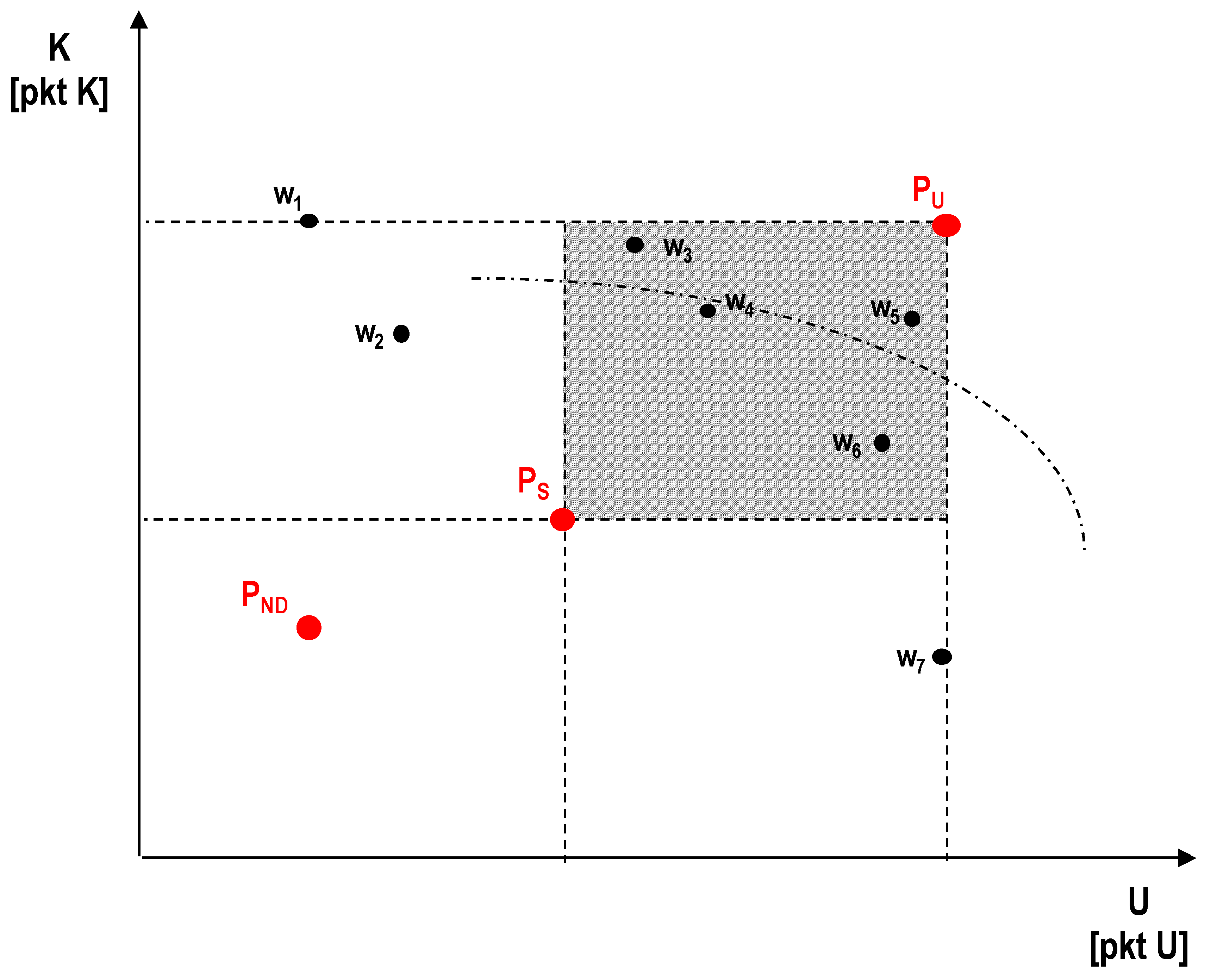
3.1. Graphic Interpretation

For further investigation, the multi-criteria issue will be reduced to a bicriteria relationship. Each previous criterion considered affects the value of the objective function and the position of the points mapping each variant. The different variants are mapped by points in a two-dimensional criterion space, in which the ordinate axis (0X) is utility and the abscissa axis (0Y) is costs (Figure 3). The utility and cost vectors are mutually perpendicular; that is, they are not cooperative.

In a set of variants, variant “x” is dominated if there is another variant in this set, for example, “y,” such that “y” is, relative to all criteria, equally or more preferred than “x.” If there is such a situation of dominance, then variant “y” is called dominant. A pair of variants “x” and “y,” in which “x” is dominated and “y” is dominant, is considered to be in a dominance relationship in the Pareto sense. It is clear that in a set containing more than two variants, the same variant can be once dominant and once dominated [55]. An alternative definition of dominance can be expressed in cone theory: a dominant point has all coordinates that are at least equal and at least one coordinate that is greater.

This method can be used to graphically represent whether a variant is optimal (non-dominated). It is enough to place the vertex of the cone at the point representing the variant to be studied and then check whether it contains any other variant. If not, it is the optimal variant, also called the optimal solution in the Pareto sense. Using the cone method, weak dominance relations can be determined. These will be points located on a plane (straight line) parallel to one of the axes [55]. Due to the restriction of the criterion space to two dimensions, the cone takes the form of a right angle “positive quadrant of the coordinate system.” Its orientation is in line with the desired directions of the objective function: utility maximization and cost minimization (increase in cost scores). In this way, Pareto-optimal solutions are identified, while the remaining points are suboptimal solutions, subject to reduction.

Figure 3. Indication of optimal variants in the Pareto sense based on the graphical (cone) method in the example of seven variants w₁–w₇; (A) study of variant w₂: w₃—strongly dominant variant, w₄—weakly dominant variant, suboptimal variant in the Pareto sense; (B) study of variant w₃: optimal variant in the Pareto sense. Source: own elaboration based on [56].

Figure 3. Indication of optimal variants in the Pareto sense based on the graphical (cone) method in the example of seven variants w₁–w₇; (A) study of variant w₂: w₃—strongly dominant variant, w₄—weakly dominant variant, suboptimal variant in the Pareto sense; (B) study of variant w₃: optimal variant in the Pareto sense. Source: own elaboration based on [56].

Additional Points in the Two-Dimensional Criterion Space, Necessary for Further Proceedings

The corner points are determined by minimizing the components of the criteria vector. These points determine the so-called utopian point—the “PU” [57]. An ideal point is usually a fictitious solution representing a set of maximum values among all achievable values in a set of solutions, but it is impossible to achieve simultaneously based on all criteria [55]. This point illustrates the maximum utility and lowest cost among the alternatives considered, which is obviously impossible for any of the variants to meet at the same time, although it indicates the possibilities of the technique and the range of costs. The PU utopian point coordinates are as follows:

• u_i—the highest utility of variant “i” (U point),
• _kj—the lowest cost of variant “j” (K point).

In the presented example, the coordinates of the utopian point are u_U—87.57 U point and k_U—94.38 K point.

For the developed method, a so-called “PND” Nadir point is also determined, representing the least-preferred level of achievement of all goals simultaneously, determined from the set of optimal points in the Pareto sense [58]:

$${\mathrm{P}}_{\mathrm{ND}}=[\min ({\mathrm{u}}_{\mathrm{io}}, \dots , {\mathrm{u}}_{\mathrm{no}}), \min ({\mathrm{k}}_{\mathrm{jo}}, \dots , {\mathrm{k}}_{\mathrm{mo}}\left)\right]$$

(26)

The P_ND Nadir point coordinates are as follows:

• u_io—utility of variant “i”, optimal in the Pareto sense (U point),
• k_io—cost of implementing variant “i”, optimal in the Pareto sense (K point).

In the presented example, the coordinates of the Nadir point are u_ND—25.48 U point and k_ND—37.49 K point.

The designer should also define the so-called “PS” satisfactory point, corresponding to the minimum technical requirements at the expected cost. The PS point coordinates are as follows:

• u_si—satisfactory utility of variant “i,”
• k_sj—satisfactory implementation costs of variant “j.”

The coordinates used in the presented example are u_S—55.00 U point and k_S—60.00 K point.

The next two points are also helpful for graphic interpretation:

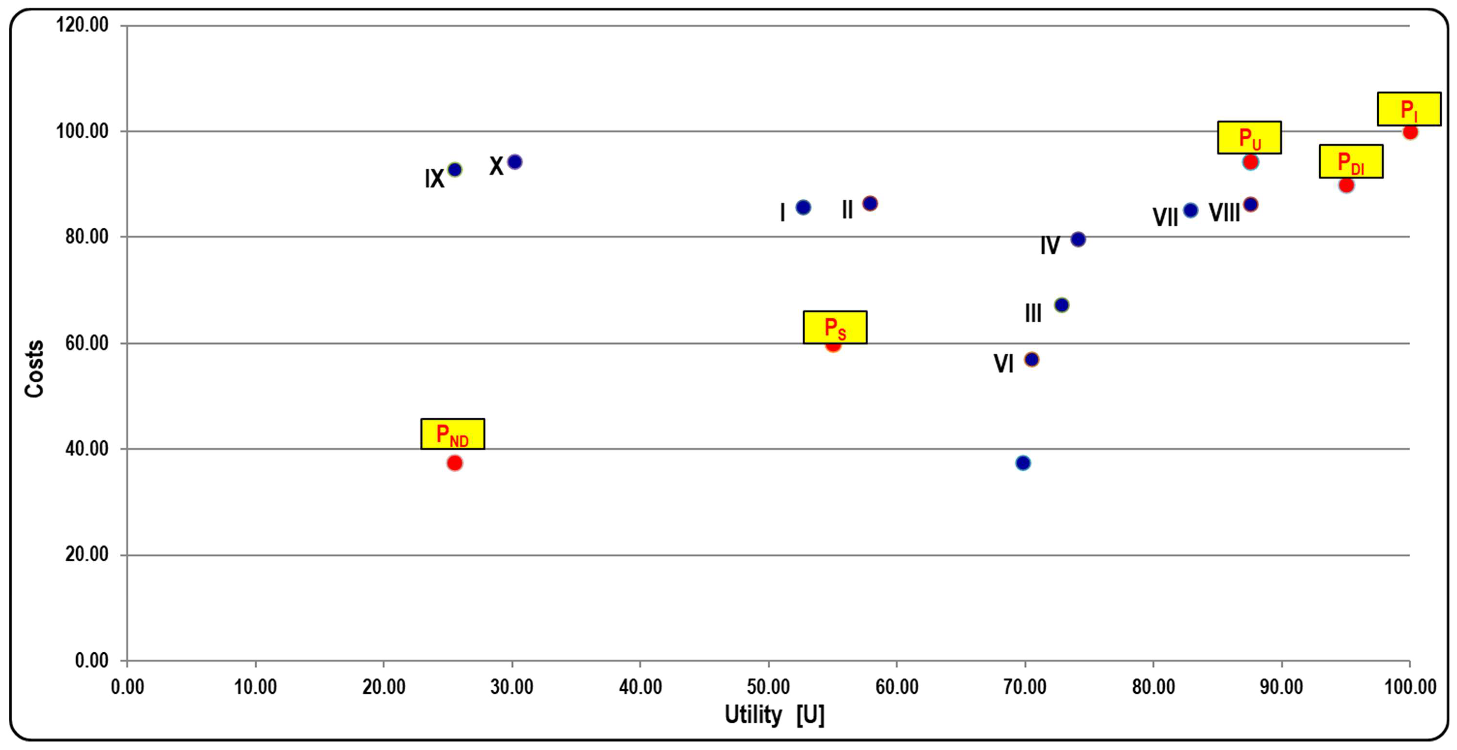
• “PI,” ideal point, constant, with coordinates of 100.00 U point and 100.00 K point,
• “PDI,” defined ideal point.

The coordinates of the defined ideal point are not determined by the coordinate values of the individual variants, but by the designer—it is a reference point reflecting the best solutions according to them [58,59]. It should be in the set determined by the “PU” utopian point and the “PS” satisfactory point with the following coordinates:

• u_DI—utility of the defined ideal variant (U point),
• k_DI—costs of the defined ideal variant (K point).

The coordinates of the “PDI” defined ideal point correspond to the variant created by defining the data at the idealized level. This point is the vertex of a new (preferred) set in the form of a rectangle, in which the opposite vertex is a satisfactory point. Analogous to the satisfactory set, solution reduction is carried out. The reduction should be carried out to avoid excessive rejection of solutions to a one-element or empty set [57].

In the presented example, the coordinate magnitudes of the “PDI” point were taken as u_DI—95.00 U point and k_DI—90.00 K point.

All of the above points are shown in

Table 10. Coordinates of additional points in the U × K bicriteria space.

Additional Points	Marking	Type	Coordinates
			Utility (U Point)	K Costs (K Point)
Utopian point	PU	Designated	87.57	94.38
Nadir point	PND	Designated	52.64	86.22
Defined satisfactory point	PDS	Determined	50.00	60.00
Defined ideal point	PDI	Determined	95.00	90.00
Ideal point	PI	Constant	100.00	100.00

Source: own elaboration.

and the following chart (Figure 4).

Figure 4 shows that the optimal variant is variant VIII.

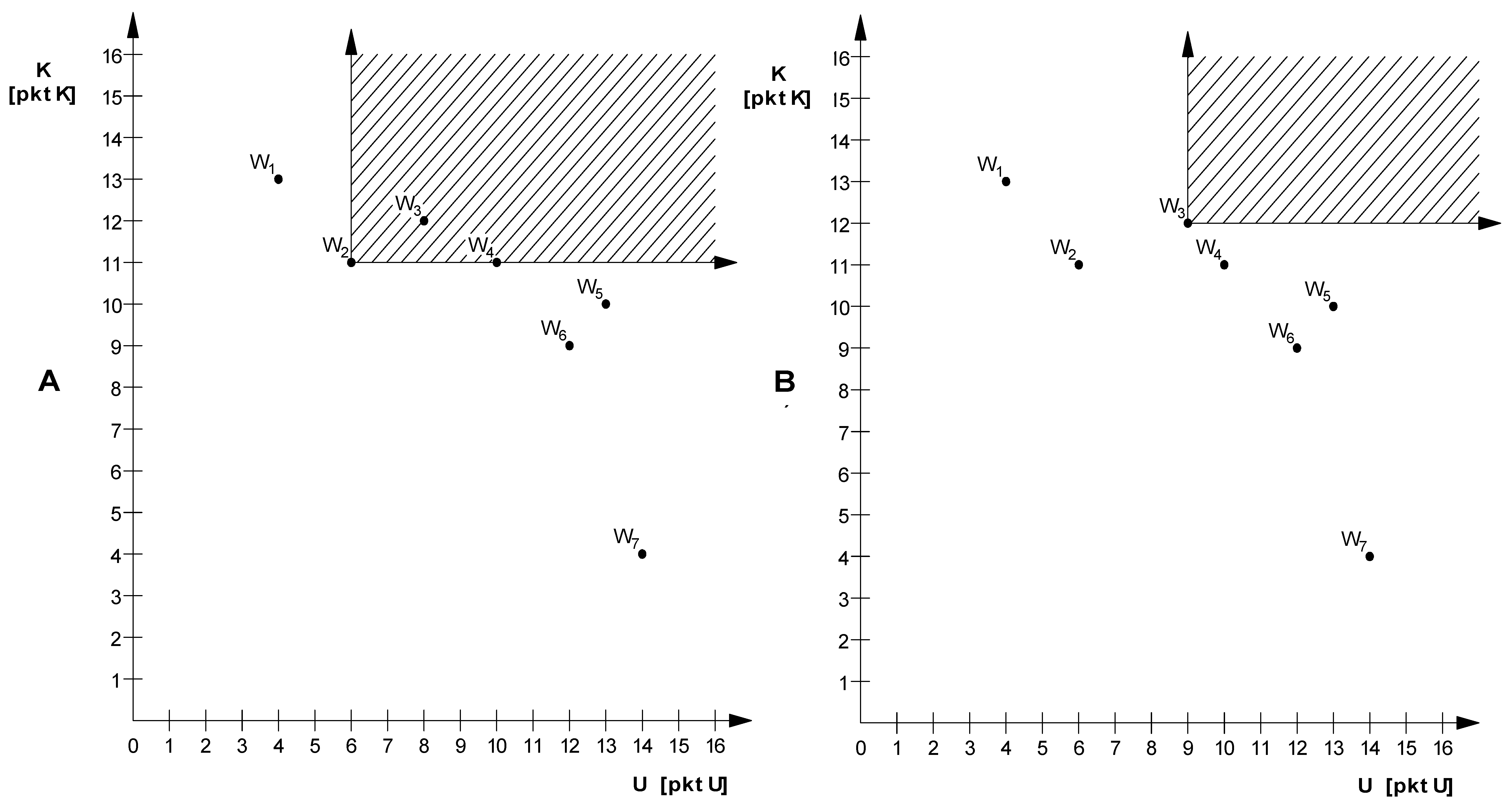
3.2. Reduction of Dominated Variants

By compiling the variants in tables and assigning to each of them the scores obtained in each criterion, it is possible to compare them with each other and thus indicate the dominance relations. In a dominance relationship, there must be a variant that is dominant over the other “w_i” variants, whose score for each criterion is higher or equal (p_ji ≥ p_jk), and is higher in at least one criterion (p_ji > p_jk). If the dominant variant in each criterion has a higher score, this is strong dominance. In other cases (when there are equal scores), it is said to be weak dominance [60].

The first reduction in the number of solution variants is the rejection of dominated variants. Their compilation should be done simultaneously in the criteria of utility and cost, as separate compilation could result in the rejection of solutions with lower utility, which at the same time could be significantly more beneficial in terms of cost.

To identify the optimal variants in the Pareto sense, each variable was tested against the others in terms of equality and dominance by comparing the size of the scores obtained. For example, for variant “i” and variant “j”:

• u_i = u_j; k_i > k_j—weak dominance of “i” over “j” (in terms of costs),
• u_i > u_j; k_i = k_j—weak dominance of “i” over “j” (in terms of utility),
• u_i > u_j; k_i > k_j—(strong) dominance of “i” over “j” (in terms of utility and cost).

The results of this procedure are presented in the form of a matrix (

Table 11. Examination of the relationship between the variants: utility–K cost mapping, row-to-column interpretation (D—dominance).

Variants	I	II	III	IV	V	VI	VII	VIII	IX	X
I	-	-	-	-	-	-	-	-	-	-
II	D	-	-	-	-	-	-	-	-	-
III	-	-	-	-	-	-	-	-	-	-
IV	-	-	D	-	-	-	-	-	-	-
V	-	-	-	-	-	-	-	-	-	-
VI	-	-	-	-	D	-	-	-	-	-
VII	-	-	D	D	D	D	-	-	-	-
VIII	D	-	-	D	D	D	D	-	-	-
IX	-	-	-	-	-	-	-	-	-	-
X	-	-	-	-	-	-	-	-	D	-

Source: own elaboration.

), in which the variants were compared one by one (rows with columns). If there was a sought-after relationship, the corresponding box (field) was filled with designations: D—dominance. No equal variants were found; that is, all the variants were distinguishable in the developed method, and only dominance relations were observed.

Table 11 shows that the optimal variants in the Pareto sense are variants VII and VIII.

3.3. Threshold Value Method

The next step is to use the threshold value method (MWP), described in the work of ref. [57], similar to the satisfaction task formulated in single- and multi-criteria optimization [61]. For this purpose, it is necessary to determine a reference point, the idea of which is presented in the works of refs. [62,63]. The concept of a reference point is to use any point in the criterion space representing the level of satisfaction of the decision-maker (designer) as a reference point in the procedure of ordering their preferences over the considered set of decision options [57]. Its role is performed by a designated satisfactory point P_S.

The method is based on narrowing down the set of satisfactory solutions within a cone (analogous to the graphical interpretation of optimal solutions in the Pareto sense) with vertices at the ideal point and an oppositely directed cone with a vertex at the satisfactory point. The common part of these sets is a rectangle with opposite vertices, which is drawn based on the Utopian point and the satisfactory point (Figure 5).

As a result, the number of solutions is reduced by discarding those outside the set determined by the rectangle. The designated “PS” satisfactory point should be between the trend line of optimal variants in the Pareto sense (if it is possible to determine it) and the Nadir point. As the trend line is approached, the level of variant reduction increases.

Using the threshold value method sets defined above, the satisfactory point and the Utopian point were determined (

Table 12. Variants belonging to the set (area) delimited by the PS and PU points.

Bicriteria Space	Variants Belonging to the PS–PU Set
U utility–K costs	II, III (zd), IV (zd), VII, VIII

zd—dominated variant. Source: own elaboration.

). Due to the small number of variants in this set, another set specified by the defined ideal point was not determined.

3.4. Distance Function

In decision support systems, the facilities under study (decision variants) are not compared with each other but are confronted with a set of reference points using superiority relations or a distance function [57]. In the field of multi-criteria optimization, the distance function is presented in the works of refs. [63,64].

A comparison of variants with a defined ideal point was used by determining the geometric distance between them according to the following formula:

$${\mathrm{d}}_{\mathrm{o}}=\mathrm{m}\mathrm{i}\mathrm{n}\sqrt{{({\mathrm{u}}_{\mathrm{D}\mathrm{I}}-{\mathrm{u}}_{\mathrm{i}})}^2+{({\mathrm{k}}_{\mathrm{D}\mathrm{I}}-{\mathrm{k}}_{\mathrm{j}})}^2}$$

(27)

where:

• d_o—distance of the tested variant from the defined ideal point,
• u_DI—utility coordinate of the defined ideal variant (U point),
• u_i—utility of the tested variant (U point),
• k_DI—cost coordinate of the defined ideal variant (K point),
• k_j—cost of the tested variant (K point).

The optimal solution will be the variant (u_i, k_j), located closest to the defined ideal point, at which the distance function reaches a minimum.

Based on Formula (27), the geometric distance in the bicriteria space of the different alternatives was determined, as shown in

Table 13. Geometric distances of individual variants from ideal points—constant and defined.

Variant	Geometric Distance from the Point
	PDI	PI
	U × K Bicriteria Space
I	42.57	49.45
II	37.25	44.19
III	31.80	42.59
IV	23.30	32.92
V	58.25	69.43
VI	41.06	52.10
VII	13.07	22.68
VIII	8.33	18.56
IX	69.58	74.86
X	64.99	70.06

Source: own elaboration.

.

In the example presented here, after comparing the point sizes of the utility and cost criteria obtained in each variant and the results of all the analyzed relationships, it can be concluded that the optimal variant for implementation will be variant VIII (

Table 14. Summary results of the analyzed relationships.

Variants
With the largest values of the product of utility and cost ratios	VIII, VII
Optimal in graphic interpretation	VIII
Non-dominated	VII, VIII
Belonging to the PS–PU set (and also non-dominated)	II, VII, VIII
Achieving minimum distance functions	VIII

Source: own elaboration.

).

4. Conclusions

Previous research and analyses of transport systems in mining focus mainly on technical and technological issues [10,11,12]), which undoubtedly serve to modernize mines but are not always a response to current and efficiency needs. In turn, management issues mainly concern transport scheduling in open-pit mines [21,22,23]. For these reasons, this methodology complements the analysis of transport issues in the investment and economic area. It is also a valuable decision-making support, which can be an effective tool in times of frequent and violent economic crises.

The developed methodology also fits into the trend of using multi-criteria analyses in mining, as postulated by Baloyi and Meyer (2020) [35]. The added value of this research is the combination of technical and economic aspects in the assessment.

The optimal variant of the designed system and configuration of the material transportation system in underground workings takes into consideration:

• seven utility criteria (KU1—transportation task completion time; KU2—compatibility of transportation systems; KU3—continuous connectivity; KU4—co-use with other transportation tasks; KU5—safety; KU6—inconvenience; KU7—operation under overplanning conditions);
• five cost criteria (KK1—costs of implementing the transportation task; KK2—costs of route expansion; KK3—rolling stock maintenance costs; KK4—depreciation costs; KK5—additional personnel costs).

Based on the aforementioned criteria, two objective functions are built for each option: utility and cost. They present divergent goals; therefore, they are non-cooperative functions. Both utility and costs strive for the maximum.

In the developed methodology, an ideal point is usually a fictitious solution representing a set of maximum values among all achievable values in a set of solutions, but it is impossible to achieve simultaneously based on all criteria. This point illustrates the maximum utility and lowest cost among the alternatives considered, which is obviously impossible for any of the variants to meet at the same time, although it indicates the possibilities of the technique and the range of costs.

The designed system for transporting materials in underground mine workings, in addition to the necessary utility qualities to ensure undisturbed operation of the ongoing mining works, should also be characterized by the optimal cost of its construction and operation. The application of the proposed cost criteria and how to use them should significantly facilitate the selection of the optimal transportation layout solution.

The simultaneous application of criteria relating to utility properties in addition to the cost criteria makes it possible to adopt a specific technical and organizational model of the subsystem of the transportation system based on the indication of the optimal solution resulting from the mathematical construction of functions of objectives relating to utility and cost. The method of selecting the optimal solution is fixed and repeatable, based on certain assumptions in which the values of the scoring weights adopted depend on the designer of the transportation subsystem in question. They can choose the optimal solution in their preferred range—either utility or cost. Thus, the model is flexible and can be adapted to different circumstances and priorities.

There are still many underground mines of hard coal and other natural resources in Poland. Taking the above circumstances into account, the following recommendations can be made regarding the use of the proposed method:

• usability and cost assessments can be carried out for existing transport systems to optimize efficiency;
• for planned transport investments, the method is ready to be implemented;
• to improve the decision-making process, the existing IT system could be equipped with solutions supporting the use of the developed methodology, e.g., obtaining information on costs or existing transport systems.

Since this paper is a scientific communication and does not include a presentation of results using a real example, in further research, the proposed approach would have to be verified in practice many times. The presentation in the article is only a demonstration of the use of the method, which is also a major research limitation of the considerations conducted. However, it should be noted that in developing the method, the authors used practical experience gathered from 13 underground mines located in the Upper Silesian Coal Basin.

Another research limitation is the use of a multi-criteria analysis. This method can be subjective. It may also not take into account all the selection criteria. However, it is holistic, carefully developed, and implementable. In the case of intuitive decisions about the selection of the transport system, the proposed method can effectively fill the existing tool gap and support the decision-making process in underground mines.

A static approach to operating conditions and cost estimation may also be a research limitation. Geological and mining conditions often change, which may have a negative impact on the level of costs. However, this will apply to all assessed variants and therefore will not influence the final decision regarding the choice of transport system.

In further research, it is worth taking into account the empirical verification of the tested method. It could also be used to evaluate and compare existing transport solutions to reduce costs and improve efficiency. An interesting research direction would also be to implement the method in underground mines extracting other mineral resources.

References

1. Szlązak, N.; Obracaj, D.; Swolkień, J. Enhancing Safety in the Polish High-Methane Coal Mines: An Overview. Min. Metall. Explor. 2020, 37, 567–579. [Google Scholar] [CrossRef]
2. Dreger, M. Variabilities in Hard Coal Production and Methane Emission in the Myslowice–Wesola Mine. J. Min. Sci. 2021, 57, 421–436. [Google Scholar] [CrossRef]
3. Wysocka, M.; Chałupnik, S.; Chmielewska, I.; Janson, E.; Radziejowski, W.; Samolej, K. Natural Radioactivity in Polish Coal Mines: An Attempt to Assess the Trend of Radium Release into the Environment. Mine Water Environ. 2019, 38, 581–589. [Google Scholar] [CrossRef]
4. Bogacz, P.; Cieślik, Ł.; Osowski, D.; Kochaj, P. Analysis of the Scope for Reducing the Level of Energy Consumption of Crew Transport in an Underground Mining Plant Using a Conveyor Belt System Mining Plant. Energies 2022, 15, 7691. [Google Scholar] [CrossRef]
5. Dubiński, J.; Prusek, S.; Turek, M.; Wachowicz, J. Hard Coal Production Competitiveness in Poland. J. Min. Sci. 2020, 56, 322–330. [Google Scholar] [CrossRef]
6. Turek, M.C.; Bednarczyk, Ł.; Jonek-Kowalska, I. Applying Utility Criteria to Select the Design Variant of the Transport System in Underground Mine Workings. Resources 2023, 12, 129. [Google Scholar] [CrossRef]
7. Kaczmarek, J.; Kolegowicz, K.; Szymla, W. Restructuring of the Coal Mining Industry and the Challenges of Energy Transition in Poland (1990–2020). Energies 2022, 15, 3518. [Google Scholar] [CrossRef]
8. Bąk, P.; Jonek-Kowalska, I. Planning the sale of hard coal in a mining enterprise: Problems and systemic solutions. In Proceedings of the 18th International Multidisciplinary Scientific GeoConference: SGEM 2018, Albena, Bulgaria, 2 July–8 July 2018; Conference proceedings, International Multidisciplinary Scientific GeoConference & EXPO SGEM, 2018, Sofia, STEF92 Technology, s.1015-1024. ISBN 978-619-7408-48-5. [Google Scholar] [CrossRef]
9. Osička, J.; Kemmerzell, J.; Zoll, M.; Lehotský, L.; Černoch, F.; Knodt, M. What’s next for the European coal heartland? Exploring the future of coal as presented in German, Polish and Czech press. Energy Res. Soc. Sci. 2020, 61, 101316. [Google Scholar] [CrossRef]
10. An, N.; Zagorščak, R.; Thomas, H.R. Transport of heat, moisture, and gaseous chemicals in hydro-mechanically altered strata surrounding the underground coal gasification reactor. Int. J. Coal Geol. 2022, 249, 103879. [Google Scholar] [CrossRef]
11. Zagorščak, R.; An, N.; Palange, R.; Green, M.; Krishnan, M.; Thomas, H.R. Underground coal gasification—A numerical approach to study the formation of syngas and its reactive transport in the surrounding strata. Fuel 2019, 253, 349–360. [Google Scholar] [CrossRef]
12. Soukup, K.; Hejtmánek, V.; Stańczyk, K.; Šolcová, O. Underground coal gasification: Rates of post processing gas transport. Chem. Pap. 2014, 68, 1707–1715. [Google Scholar] [CrossRef]
13. Tu, J.; Wan, L.; Sun, Z. Safety Improvement of Sustainable Coal Transportation in Mines: A Contract Design Perspective. Sustainability 2023, 15, 2085. [Google Scholar] [CrossRef]
14. Li, J.; Yang, Y.; Li, J.; Mao, Y.; Saini, V.; Kokh, S. A TGA–DSC-based study on macroscopic behaviors of coal–oxygen reactions in context of underground coal fires. J. Therm. Anal. Calorim. 2022, 147, 3185–3194. [Google Scholar] [CrossRef]
15. Fabiano, B.; Currò, F.; Reverberi, A.P.; Palazzi, E. Coal dust emissions: From environmental control to risk minimization by underground transport. An applicative case-study. Process Saf. Environ. Prot. 2014, 92, 150–159. [Google Scholar] [CrossRef]
16. Thakur, P. Gas Transport in Underground Coal Mines. Adv. Mine Vent. Respirable Coal Dust Combust Gas Mine Fire Control 2019, 299–312. [Google Scholar] [CrossRef]
17. Wang, M.; Bao, J.; Yuan, X.; Yin, Y.; Khalid, S. Research Status and Development Trend of Unmanned Driving Technology in Coal Mine Transportation. Energies 2022, 15, 9133. [Google Scholar] [CrossRef]
18. Yuan, X.; Bi, Y.; Hao, M.; Ji, Q.; Liu, Z.; Bao, J. Research on Location Estimation for Coal Tunnel Vehicle Based on Ultra-Wide Band Equipment. Energies 2022, 15, 8524. [Google Scholar] [CrossRef]
19. Krauze, K.; Mucha, K.; Wydro, T.; Klempka, R.; Kutnik, A.; Hałas, W.; Ruda, P. Determining the Stability of a Mobile Manipulator for the Transport and Assembly of Arches in the Yielding Arch Support. Energies 2022, 15, 3170. [Google Scholar] [CrossRef]
20. Szewerda, K.; Tokarczyk, J.; Wieczorek, A. Impact of Increased Travel Speed of a Transportation Set on the Dynamic Parameters of a Mine Suspended Monorail. Energies 2021, 14, 1528. [Google Scholar] [CrossRef]
21. Zhang, Z.; Zhang, R.; Sun, J. Research on the Comprehensive Evaluation Method of Driving Behavior of Mining Truck Drivers in an Open-Pit Mine. Appl. Sci. 2023, 13, 11597. [Google Scholar] [CrossRef]
22. Teplická, K.; Khouri, S.; Beer, M.; Rybárová, J. Evaluation of the Performance of Mining Processes after the Strategic Innovation for Sustainable Development. Processes 2021, 9, 1374. [Google Scholar] [CrossRef]
23. Fang, Y.; Peng, X. Micro-Factors-Aware Scheduling of Multiple Autonomous Trucks in Open-Pit Mining via Enhanced Metaheuristics. Electronics 2023, 12, 3793. [Google Scholar] [CrossRef]
24. Ren, X.; Guo, H.; Sheng, K.; Mao, G. Real-Time Path Planning of Driverless Mining Trains with Time-Dependent Physical Constraints. Appl. Sci. 2023, 13, 3729. [Google Scholar] [CrossRef]
25. Krysa, Z.; Bodziony, P.; Patyk, M. Discrete Simulations in Analyzing the Effectiveness of Raw Materials Transportation during Extraction of Low-Quality Deposits. Energies 2021, 14, 5884. [Google Scholar] [CrossRef]
26. Halilović, D.; Gligorić, M.; Gligorić, Z.; Pamučar, D. An Underground Mine Ore Pass System Optimization via Fuzzy 0–1 Linear Programming with Novel Torricelli–Simpson Ranking Function. Mathematics 2023, 11, 2914. [Google Scholar] [CrossRef]
27. Steuer, R.E. Multiple Criteria Optimization: Theory, Computation and Application; John Wiley: New York, NY, USA, 1986. [Google Scholar]
28. Köksalan, M.M.; Wallenius, J.; Zionts, S. Multiple Criteria Decision Making: From Early History to the 21st Century; World Scientific: Singapore, 2011. [Google Scholar]
29. Sahoo, S.K.; Goswami, S.S. A Comprehensive Review of Multiple Criteria Decision-Making (MCDM) Methods: Advancements, Applications, and Future Directions. Decis. Mak. Adv. 2023, 1, 25–48. [Google Scholar] [CrossRef]
30. Li, X.; Cao, Z.; Xu, Y. Characteristics and trends of coal mine safety development. Energy Sources Part A Recovery Util. Environ. Eff. 2020. [Google Scholar] [CrossRef]
31. Kong, B.; Cao, Z.; Sun, T.; Qi, C.; Zhang, Z. Safety hazards in coal mines of Guizhou China during 2011–2020. Saf. Sci. 2022, 145, 105493. [Google Scholar] [CrossRef]
32. Namin, F.S.; Ghadi, A.; Saki, S. A literature review of Multi-Criteria Decision-Making (MCDM) towards mining method selection (MMS). Resour. Policy 2022, 77, 102676. [Google Scholar] [CrossRef]
33. Sitorus, F.; Cilliers, J.J.; Brito-Parada, P.R. Multi-criteria decision making for the choice problem in mining and mineral processing: Applications and trends. Expert Syst. Appl. 2019, 121, 393–417. [Google Scholar] [CrossRef]
34. Hao, M.; Nie, Y. Hazard identification, risk assessment and management of industrial system: Process safety in mining industry. Saf. Sci. 2022, 154, 105863. [Google Scholar] [CrossRef]
35. Baloyi, V.D.; Meyer, L.D. The development of a mining method selection model through a detailed assessment of multi-criteria decision methods. Results Eng. 2020, 8, 100172. [Google Scholar] [CrossRef]
36. Jiskani, I.M.; Cai, Q.; Zhou, W.; Lu, X.; Shah, S.A.A. An integrated fuzzy decision support system for analyzing challenges and pathways to promote green and climate-smart mining. Expert Syst. Appl. 2022, 188, 116062. [Google Scholar] [CrossRef]
37. Jiskani, I.M.; Wei, Z.; Shahab, H.; Zhiming, W. Mining 4.0 and climate neutrality: A unified and reliable decision system for safe, intelligent, and green & climate-smart mining. J. Clean. Prod. 2023, 41015, 137313. [Google Scholar] [CrossRef]
38. Chen, J.; Jiskani, I.M.; Lin, A.; Zhao, C.; Jing, P.; Liu, F.; Lu, M. A hybrid decision model and case study for comprehensive evaluation of green mine construction level. Environ. Dev. Sustain. 2023, 25, 3823–3842. [Google Scholar] [CrossRef]
39. Erzurumlu, S.S.; Erzurumlu, Y.O. Sustainable mining development with community using design thinking and multi-criteria decision analysis. Resour. Policy 2015, 46, 6–14. [Google Scholar] [CrossRef]
40. Matuszewicz, J. Rachunek Kosztów; Wydawnictwo Finans-Servis: Warszawa, Poland, 2011. [Google Scholar]
41. Jonek-Kowalska, I. Zarządzanie Kosztami w Przedsiębiorstwach Górniczych w Polsce. Stan Aktualny i Kierunki Doskonalenia; Wydawnictwo Difin: Warszawa, Poland, 2013. [Google Scholar]
42. Bąk, P. Production planning in a mining enterprise—Selected problems and solutions. Gospod. Surowcami Miner.—Miner. Resour. Manag. 2018, 24, 97–116. [Google Scholar] [CrossRef]
43. Michalak, A.; Jonek-Kowalska, I. Ryzyko, Koszt Kapitału i Efektywność w Procesie Finansowania Inwestycji Rozwojowych w Górnictwie Węgla Kamiennego; Wydawnictwo Naukowe PWN: Warszawa, Poland, 2011. [Google Scholar]
44. Michalak, A.; Jonek-Kowalska, I. Finansowanie Inwestycji Rozwojowych w Górnictwie Węgla Kamiennego a Wartość Przedsiębiorstw Górniczych; Wydawnictwo Naukowe PWN: Warszawa, Poland, 2011. [Google Scholar]
45. Jonek-Kowalska, I. Long-term Analysis of the Effects of Production Management in Coal Mining in Poland. Energies 2019, 12, 3146. [Google Scholar] [CrossRef]
46. Jonek-Kowalska, I. Method for Assessing the Development of Underground Hard Coal Mines on a Regional Basis: The Concept of Measurement and Research Results. Energies 2018, 11, 1370. [Google Scholar] [CrossRef]
47. Jonek-Kowalska, I.; Turek, M. Dependence of Total Production Costs on Production and Infrastructure Parameters in the Polish Hard Coal Mining Industry. Energies 2017, 10, 1480. [Google Scholar] [CrossRef]
48. Sadowy, J. Kryteria Oceny Ofert w Postępowaniu o Udzielnie Zamówienia Publicznego—Przykłady Zastosowania; Urząd Zamówień Publicznych: Warszawa, Poland, 2011. [Google Scholar]
49. Koba, A. Pozacenowe Kryteria Oceny Ofert. Poradnik z Katalogiem Dobrych Praktyk; Urząd Zamówień Publicznych: Warszawa, Poland, 2013. [Google Scholar]
50. Urbanyi-Popiołek, I. Ekonomiczne i Organizacyjne Aspekty Transportu; Wydawnictwo Uczelniane Wyższej Szkoły Gospodarki w Bydgoszczy: Bydgoszcz, Poland, 2013. [Google Scholar]
51. Karwowski, T. Zasady Eksploatacji i Opłacalności Zakupu Maszyn; IBMiER: Warszawa, Poland, 1996. [Google Scholar]
52. Iwin-Garzyńska, J. Kapitał Amortyzacyjny w Zarzadzaniu Finansami; Polskie Wydawnictwo Ekonomiczne: Warszawa, Poland, 2016. [Google Scholar]
53. Michalak, A. Parametry efektywności w cyklu życia inwestycji. Zesz. Nauk. Politech. Śląskiej Ser. Organ. I Zarządzanie 2013, 66. Available online: https://delibra.bg.polsl.pl/dlibra/publication/85272/edition/75875/content (accessed on 30 November 2023).
54. Kaliszewski, I. Wielokryterialne Podejmowanie Decyzji; Wydawnictwo Naukowo-Techniczne: Warszawa, Poland, 2008. [Google Scholar]
55. Cegiełka, K. Matematyczne Wspomaganie Decyzji; Szkoła Główna Służby Pożarniczej: Warszawa, Poland, 2012. [Google Scholar]
56. Montusiewicz, J. Ewolucyjna analiza wielokryterialna w zagadnieniach technicznych. Pr. Inst. Podstawowych Probl. Tech. PAN 2004, 5. Available online: https://www.infona.pl/resource/bwmeta1.element.baztech-article-BPB4-0018-0006 (accessed on 30 November 2023).
57. Montusiewicz, J. Wspomaganie Procesów Projektowania i Planowania Wytwarzania w Budowie i Eksploatacji Maszyn Metodami Analizy Wielokryterialnej; Wydawnictwo Politechniki Lubelskiej: Lublin, Poland, 2012. [Google Scholar]
58. Coello Coello, C.A.; Christiansen, A.D. A Multiobjective Optimization Tool for Engineering Design. Eng. Optim. 1999, 31, 337–368. [Google Scholar] [CrossRef]
59. Kliber, P. Wprowadzenie Do Teorii Gier. Materiały Dydaktyczne; Wydawnictwo Uniwersytetu Ekonomicznego w Poznaniu: Poznań, Poland, 2015. [Google Scholar]
60. Paszkowski, S. Podstawy Teorii Systemów i Analizy Systemowej; Wydawnictwo Wojskowej Akademii Technicznej: Warszawa, Poland, 1999. [Google Scholar]
61. Konarzewska-Gubała, E. Wspomaganie decyzji wielokryterialnych: System BIPOLAR; Uniwersytet Ekonomiczny We Wrocławiu: Wrocław, Poland, 1991; Volume 76. [Google Scholar]
62. Skolimowski, A.M. Decision Support Systems Based on Reference Sets. Rozprawy i Monografie, nr 40; Wydawnictwa AGH: Kraków, Poland, 1996. [Google Scholar]
63. Galas, Z.; Nykowski, I.; Żółkiewski, Z. Programowanie Wielokryterialne; Państwowe Wydawnictwo Naukowe: Warszawa, Poland, 1987. [Google Scholar]
64. Salukwadze, M.E. Мнoгoкритериальные задачи oптимизации в теoрии oптимальных улучшений; Miecniereba: Tibilisi, Gruzja, 1975. [Google Scholar]
Figure 1. Research stages: selection of the optimal transport system.
Resources 13 00014 g001
Figure 2. Variants—the product of utility rates U and costs K.
Resources 13 00014 g002
Figure 4. Graphic interpretation of individual variants and additional points in the bicriteria space of U utility–K cost. Source: own elaboration.
Resources 13 00014 g004
Figure 5. Additional points of the two-dimensional criterion space U (utility), K (cost), with example variants w1–w7 along with the trend line PU—utopian point, PND—Nadir point, PS—satisfactory point, reduction of variants w1, w2, and w7 located outside the area defined by points PU and PS. Source: own elaboration based on ref. [57].
Resources 13 00014 g005