Article

Signal Filtering Using Neuromorphic Measurements

1
Department of Electrical and Electronic Engineering, Imperial College London, London SW7 2AZ, UK
2
School of Engineering, Newcastle University, Newcastle upon Tyne NE1 7RU, UK
*
Authors to whom correspondence should be addressed.
J. Low Power Electron. Appl. 2023, 13(4), 63; https://doi.org/10.3390/jlpea13040063
Submission received: 18 October 2023 / Revised: 22 November 2023 / Accepted: 30 November 2023 / Published: 6 December 2023

Abstract

:
Digital filtering is a fundamental technique in digital signal processing, which operates on a digital sequence without any information on how the sequence was generated. This paper proposes a methodology for designing the equivalent of digital filtering for neuromorphic samples, which are a low-power alternative to conventional digital samples. In the literature, filtering using neuromorphic samples is performed by filtering the reconstructed analog signal, which is required to belong to a predefined input space. We show that this requirement is not necessary, and introduce a new method for computing the neuromorphic samples of the filter output directly from the input samples, backed by theoretical guarantees. We show numerically that we can achieve a similar accuracy compared to that of the conventional method. However, given that we bypass the analog signal reconstruction step, our results show significantly reduced computation time for the proposed method and good performance even when signal recovery is not possible.

1. Introduction

In contemporary computing, the majority of tasks necessitate some form of digital signal processing [1]. With the escalating computational capabilities of digital processing systems, there is a concurrent surge in power consumption. This is further exacerbated by the rapid advancements in the field of artificial intelligence. Neuromorphic sampling, or time encoding, is an alternative to traditional digital encoding that transforms an analog signal into a sequence of low-power time-based pulses, often referred to as a spike train. Neuromorphic sampling draws its inspiration from neuroscience and introduces a paradigm shift by significantly reducing power consumption during encoding and transmission [2,3]. Despite these advantages, as of now, there exist no equivalents of digital signal processing operations tailored to neuromorphic sampling. This unexplored territory holds the promise of groundbreaking developments in low-power and efficient signal processing.
In this paper, we address the problem of filtering a signal using its neuromorphic measurements, thus extending the principle of digital signal filtering for the case of neuromorphic sampling. In posing this problem, we do not seek alternatives for spiking neural networks, but rather theoretically validated analytical approaches. Moreover, the proposed problem is not to replace existing conventional digital signal processing, but it is posed under the assumption that the communication protocol is emitting and receiving spike trains [4,5]. In this case, the proposed problem is to perform the mathematical operation of filtering on the analog signals encoded in these spike trains.
In the literature, the concept of spike train filtering predominantly refers to convolving the filter function with a sequence of Diracs centered in the spike times [6]. This is not an operation on the analog signal that resulted in those neuromorphic samples. Moreover, in the context of neuromorphic measurements generated from multidimensional signals, such as those generated by event cameras [7], filtering also refers to performing multidimensional spatial convolution [8,9]. The case of filtering the analog signal via its neuromorphic measurements was proposed in [10], but the process also involves signal reconstruction. A filtering approach of neuromorphic signals without reconstruction was first studied in [11].
Therefore, conventionally, to process the signal underlying a sequence of spike measurements, the signal is recovered in the analog domain, followed by filtering and neuromorphic sampling. There are a number of drawbacks with this approach. First, this method does not exploit the power consumption advantage of neuromorphic measurements. Second, this approach is heavier computationally due to the complexity of signal reconstruction from neuromorphic samples [12,13]. Third, reconstruction is only possible if the input satisfies some restrictive smoothness or sparsity constraints. However, for conventional sampling, the process of digital filtering is independent of the charateristics of the signal that generated the measurements.
In this paper, we derive a direct mapping between the time encoded inputs and outputs of an analog filter. The proposed mapping forms the basis for a practical filtering algorithm of the underlying signal corresponding to some given neuromorphic measurements, without direct access to the signal. We introduce theoretical guarantees and error bounds for the measurements generated with the proposed algorithm. Through numerical simulations, we demonstrate the performance of our method in terms of speed, but also reduced restrictions on the input signal, in comparison with the existing conventional method.
This paper is structured as follows. Section 2 presents a brief review of the time encoding model used in this paper and associated input reconstruction methods. Section 3 introduces the proposed problem. Section 4 describes the proposed filtering method. Numerical results are presented in Section 5. Section 6 presents the concluding remarks.

2. Time Encoding

The time encoding machine (TEM) is a conceptualization of neuromorphic sampling that maps input u ( t ) into sequence of samples t k k Z . The particular TEM considered here is the integrate-and-fire (IF) TEM, which is inspired by neuroscience. Consequently, sequence t k k Z is called a spike train, where the spike refers to the firing of an action potential, representing the information transmission method in the mammalian cortex. Previously, the IF model was used for system identification of biological neurons [14,15] to perform machine learning tasks [16,17] but also for input reconstruction [13,18,19,20,21]. The IF model adds input g ( t ) with bias parameter b, and subsequently integrates the output to generate a strictly increasing function y ( t ) . When y ( t ) crosses threshold δ , the integrator is reset and the IF generates output spike time t k . The IF TEM is described by the following equations:
t k t k + 1 u ( s ) d s = δ b t k + 1 t k , k Z + * .
Without reducing the generality, it is assumed that t 0 = 0 . A common assumption is that the input is bounded by c R + , such that u ( t ) c < b . This bound enables derivation of the following density guarantees [2]:
δ b + c t k + 1 t k δ b c .
Signal u ( t ) is, in the general case, not recoverable from t k k Z . To ensure it can be reconstructed, we require imposing restrictive assumptions. A common assumption is that u ( t ) belongs to P W Ω , the space of functions bandlimited to Ω rad / s that are also square integrable, i.e., u L 2 R . If this assumption is satisfied, then u ( t ) can be recovered from t k k Z if
δ b c < π Ω .
To ofer an intuition on the recovery condition and its link to the Nyquist rate, we note that TEM Equation (1) can be re-written as
u , 1 t k , t k + 1 L 2 = δ b t k + 1 t k ,
where · , · L 2 denotes the inner product in Hilbert space L 2 R of square integrable functions and 1 t k , t k + 1 is the characteristic function of t k , t k + 1 . We note that although 1 t k , t k + 1 L 2 R , it is not bandlimited, i.e., 1 t k , t k + 1 P W Ω . However, due to the properties of the inner product [22],
u , 1 t k , t k + 1 L 2 = u , φ k L 2 = δ b t k + 1 t k ,
where φ k ( t ) sin Ω · π · 1 t k , t k + 1 ( t ) denotes the projection of 1 t k , t k + 1 in P W Ω . In the case of the Nyquist rate condition, the uniform samples can be described as
u ( k T ) = u , sin Ω · k T π · k T L 2 .
The Nyquist rate criterion [23] ensures that u ( k T ) k Z uniquely identify u ( t ) if T < π Ω , which is guaranteed by the fact that functions sin Ω · k T π · k T k Z form a basis in P W Ω . The same is not true in the case of time encoding, which is a form of nonuniform sampling [24,25,26], where φ k k Z do not form a basis. They can, however, form the more general concept of frame [27], which guarantees that u ( t ) is uniquely determined by u , φ k L 2 if sequence t k k Z is dense enough. Via (2), we can use δ b c as a measure of density of sequence t k k Z , yielding Nyquist-like criterion (3).
Input u ( t ) is then recovered from t k k Z as
u ( t ) = m Z c ˜ m · sin Ω t s k π t s k ,
where s k = t k + t k + 1 2 are the midpoints of intervals t k , t k + 1 and c ˜ k are the solution in the least square sense of the following system [22]:
n Z c n t k t k + 1 sin Ω t s k π t s k d t = δ b t k + 1 t k .
Unlike uniform sampling, the input recovery for an IF TEM is much more complex computationally because, for each new input, functions sin Ω t s k π t s k have to be computed and System (6) needs to be solved. This becomes very demanding computationally for long sequences t k . Alternative recovery approaches are based on optimizing a smoothness-based criterion instead of aiming to uniquely recover the input [28,29]. Moreover, the problem of input recovery was shown to be equivalent to that of system identification of a filter in series with an IF TEM in the case of linear [30,31] and nonlinear filters [32].
The methods presented so far are assuming the input is bandlimited. Further generalizations were introduced for the case where u ( t ) is a function in a shift-invariant space [13,19] or in a space with finite rate of innovation [20,21]. However, if u ( t ) does not belong to one of the classes above, or if it is bandlimited and does not satisfy (3), then the conventional theory does not allow any processing of signal u ( t ) via its samples t k . The same is not true for conventional digital signals, which can be processed even when they are not sampled at the Nyquist rate. We show that some types of processing such as filtering are still doable even when (3) is not true.

3. Problem Statement

Here, we formulate the proposed signal filtering problem as follows. We assume the neuron input is continuous, i.e., u C R . To satisfy the neuron encoding requirement in Section 2, we assume the input is bounded, such that u t c < b , t R . Furthermore, we assume that the input is absolutely integrable u L 1 ( R ) and square integrable u L 2 ( R ) . Following the same idea as in digital filtering, we do not impose any general conditions on the bandwidth, smoothness, or sparsity of the analog signal in order to compute the filter output.
The filter is assumed to be linear, with impulse response g ( t ) that is continuous, g C R , and absolutely integrable, g L 1 ( R ) . The output of the filter then satisfies
y t = u τ g t τ d τ , y t u τ · g t τ d τ c g L 1 c ,
where the last inequality assumes that g L 1 1 , which is introduced to ensure that y ( t ) c , which in turn allows y ( t ) sampling by the same neuron. According to the properties of the convolution operator, we also have y L 2 ( R ) L 1 R , where L 2 ( R ) denotes the space of square integrable functions.
We let t k u k Z and t k y k Z be the neuromorphic samples of signals u and y, respectively, computed using an IF neuron with parameters δ , b . The proposed problem is to compute t k y knowing t k u , sampling parameters δ , b and filter g ( t ) . This problem, illustrated in Figure 1, is inspired by digital signal processing, where a digital filter is applied directly to the samples of a signal. The conventional way to address this problem would be to recover u ( t ) from t k u , apply filter g ( t ) in the analog domain, and subsequently sample output y ( t ) with the same IF model to obtain t k y . We refer to this as the indirectmethod for filtering. The first step of recovery, however, is not possible unless we impose some further restrictive conditions on u ( t ) such as being bandlimited [22], shift-invariant [13,19], or having a finite rate of innovation [18,20]. Therefore, the proposed problem is not solvable in its full generality using conventional approaches.
However, if we replace neuromorphic sampling by conventional uniform sampling, this problem leads to the widely used operation of digital filtering. The operation itself does not require any special conditions on the analog signal that generated these samples. Therefore, an equivalent of this solution for the case of neuromorphic sampling is highly desirable.

4. The Proposed Neuromorphic Direct Filtering Method

In this section, we describe the proposed direct filtering method. To compute t k y from t k u we need to create an analytical link between the integrals of the underlying analog signals u ( t ) and y ( t ) due to the integral operators in (1) and (7). To this end, we define the following auxiliary functions:
U t 0 t u τ d τ , Y t 0 t y τ d τ .
We note that U satisfies U t u L 1 . Using Young’s convolution inequality, we obtain Y t y L 1 u L 1 · g L 1 . Using these functions, we derive the equivalent of t-transform Equations (1) as
U ( t k u ) = k δ b t k u , Y ( t k y ) = k δ b t k y , k Z .
Assuming we know Y ( t ) , the target spike train t k y satisfies f k ( t k y ) = t k y , where
f k ( t ) 1 b k δ Y ( t ) .
The following result shows that t k y can be uniquely computed using f k ( t ) .
Lemma 1
(Exact Output Samples Computation). Function f k ( t ) has a unique fixed point t = t k y . Furthermore, we let t k , m y be computed recursively such that t k , 0 y R is arbitrary and
t k , m + 1 y = f k t k , m y .
Then, lim m t k , m y = t k y and t k , m y t k y < t k y t k , 0 y c b m .
Proof. 
We assume, by contradiction, that t ¯ t k y such that f k ( t ¯ ) = t ¯ . It follows that
b t ¯ + Y ( t ¯ ) = 0 t ¯ y ( τ ) + b d τ = k δ .
On the other hand, we know that y ( t ) c < b due to (7), and thus 0 t ¯ y ( τ ) + b d τ is a strictly increasing function of t ¯ , which ensures that 0 t ¯ y ( τ ) + b d τ = k δ has a unique solution. Using (9), we obtain t ¯ = t k y , which invalidates our initial assumption and proves uniqueness.
From (9), it follows that k Z , f k ( t k y ) = t k y . The following holds:
f k t = y t b c b ,
and thus
ζ 0 , t t k y ζ , t k y + ζ , f k t t k y ζ c b , t k y + ζ c b .
We let ζ = t k y t k , 0 y and t = t k , 0 y . It follows that
f k ( t k , 0 y ) t k y = t k , 1 y t k y t k y t k , 0 y c b .
Similarly, by choosing ζ = t k y t k , 1 y and t = t k , 1 y , we obtain
t k y t k , 2 y t k y t k , 1 y c b t k y t k , 0 y c b 2 ,
and the process continues recursively, which completes the proof via c < b .  □
Therefore, t k y can be computed by solving the fixed-point equation f k ( t ) = t . This equation requires knowing Y ( t ) , which satisfies
Y t = 0 t g τ u s τ d τ d s = g τ 0 t u s τ d s d τ = g τ [ U ( t τ ) U ( τ ) ] d τ = U τ [ g ( t τ ) g ( τ ) ] d τ ,
where the last equality uses the variable change τ t τ . In reality, however, Y ( t ) is unknown, since it could only be precisely computed using U ( t ) . Given that we only know t k u and do not impose any smoothness or sparsity conditions on u ( t ) , we do not have access to U ( t ) , but only to its samples U t k u via (9). In the following, we show that Y ( t ) , f k ( t ) and subsequently t k y can be estimated using a piecewise constant approximation of U ( t ) at points t k u . We let f ˜ k : R R be defined by
f ˜ k ( t ) = 1 b k δ Y ˜ ( t ) ,
where
Y ˜ t = I 1 U τ g t τ g τ d τ ,
where I 1 U ( t ) is the piecewise constant interpolant to U at points t k u k Z , such that I 1 U ( t ) = U t k u for t t k u , t k + 1 u . The next proposition derives some properties of Y ˜ t .
Proposition 1.
Function Y ˜ t is continuous and satisfies
Y ˜ t = k Z U t k u G ( t t k u ) + G ( t k u ) U t k u G ( t t k + 1 u ) G ( t k + 1 u ) ,
where G ( t ) 0 t g ( s ) d s .
Proof. 
Using (15), we obtain
Y ˜ ( t ) = k Z t k u t k + 1 u I 1 U τ g t τ g τ d τ = k Z U t k u t k u t k + 1 u g ( t τ ) d τ t k u t k + 1 u g ( τ ) d τ = k Z U t k u t t k + 1 u t t k u g ( τ ) d τ t k + 1 u t k u g ( τ ) d τ ,
which proves (16). It follows that Y ˜ ( t ) is a linear combination of continuous functions; thus, it is itself continuous.  □
Proposition 1 shows that, unlike Y ( t ) and f k ( t ) , function Y ˜ ( t ) and, consequently, also f ˜ k ( t ) , are fully known from the IF parameters and input samples t k u . The remaining challenge is to show that the fixed point equation f ˜ k ( t ) = t can be solved and to provide an error bound for estimating t k y . This challenge is addressed rigorously in the next theorem. Moreover, the result allows computing recursively a sequence of estimations t ˜ k , m y that converges to a vicinity of t k y .
Theorem 1
(Estimating Output Samples from Input Samples). We let u ( t ) be a signal satisfying u L 1 R L 2 R C ( R ) , u t c < b . Furthermore, we let g ( t ) be the impulse response of a filter satisfying g L 1 R C R , g L 1 1 , and let y ( t ) be the filter output in response to input u ( t ) . Signals u ( t ) and y ( t ) , sampled with an IF neuron with parameters δ , b , generate values t k u k Z and t k y k Z , respectively. Then, the following hold true:
(a) 
k Z , t ˜ k y t k y 2 δ c b c 2 , t k y + 2 δ c b c 2 such that f ˜ k ( t ˜ k y ) = t ˜ k y , where f ˜ k ( t ) satisfies (14).
(b) 
We let t ˜ k , m y be a sequence defined recursively as t ˜ k , m + 1 y = f ˜ k ( t ˜ k , m y ) , where t ˜ k , 0 y R . Then,
t ˜ k , m y t k y t k y t ˜ k , 0 y · c b m + 2 δ c b ( b c ) · i = 1 m c b i 1 .
(c) 
For t ˜ k , m y defined above, m 0 Z such that t ˜ k , m y t k y 2 δ c b c 2 , t k y + 2 δ c b c 2 , m > m 0 .
Proof. 
( a ) Function Y ˜ satisfies
Y t Y ˜ t U τ I 1 U ( τ ) · g t τ g τ d τ Δ · sup τ R U ( τ ) · g t τ g τ d τ E ,
where E = 2 Δ c g L 1 , Δ = s u p k Z t k + 1 u t k u . From (12), the following holds:
ζ 0 , t t k y ζ , t k y + ζ , f k t t k y ζ c b , t k y + ζ c b .
Using f k t f ˜ k t E b , t R ,
ζ 0 , t t k y ζ , t k y + ζ , f k ˜ t t k y ζ c b E b , t k y + ζ c b + E b .
Unlike in the case of Lemma 1, in this case, applying f k ˜ ( t ) recursively does not guarantee the exact computation of t k y . However, we observe that by picking ζ = E b c , we obtain identical intervals for t and f k ˜ ( t ) :
t t k y E b c , t k y + E b c , f k ˜ t t k y E b c , t k y + E b c .
This observation is very useful as it enables applying Brouwer’s fixed-point theorem which states that for any continuous function f : S S where S is a nonempty compact convex set, there is a point t 0 such that f ( t 0 ) = t 0 . Given that Y ˜ ( t ) is continuous due to Proposition 1, it follows that f ˜ k is also continuous. By applying Brouwer’s fixed point theorem for f ( t ) = f ˜ k ( t ) and S = t k y E b c , t k y + E b c , it follows that f k ( t ) has a fixed point in S . We recall that E = 2 Δ c g L 1 , which, using (2), leads to
E 2 δ c b c g L 1 2 δ c b c .
It follows that S t k y 2 δ c b c 2 , t k y + 2 δ c b c 2 , which yields the required result.
( b ) We approach this proof using mathematical induction. We select t = t ˜ k , 0 y in (21). Using (23), it follows that
f ˜ k t ˜ k , 0 y t k y ζ c b + 2 δ c b ( b c ) , s . t . t ˜ k , 0 y t k y ζ , t k y + ζ .
We note that t ˜ k , 0 y t k y ζ , t k y + ζ is always true for ζ = t k y t ˜ k , 0 y , which yields
f ˜ k t ˜ k , 0 y t k y t k y t ˜ k , 0 y c b + 2 δ c b ( b c ) .
This demonstrates that (18) is true for m = 1 . To finalize the induction, we assume (18) to be true, and show it is true for m + 1 as follows:
t ˜ k , m + 1 y t k y = f ˜ k t ˜ k , m y t k y ζ c b + 2 δ c b ( b c ) .
Finally, as before, we use the fact that ζ = t k y t ˜ k , m y guarantees t ˜ k , m y t k y ζ , t k y + ζ . We also use the fact that ζ is bounded by (18), which, when substituted in (26), leads to the desired result via (23).
(c) Equation (18) can be expanded into
t ˜ k , m y t k y + t k y t ˜ k , 0 y c b m + 2 δ c ( b c ) 2 · 1 c b m ,
t ˜ k , m y t k y t k y t ˜ k , 0 y c b m 2 δ c ( b c ) 2 · 1 c b m .
The required result follows from lim m c b m = 0 via (23).   □
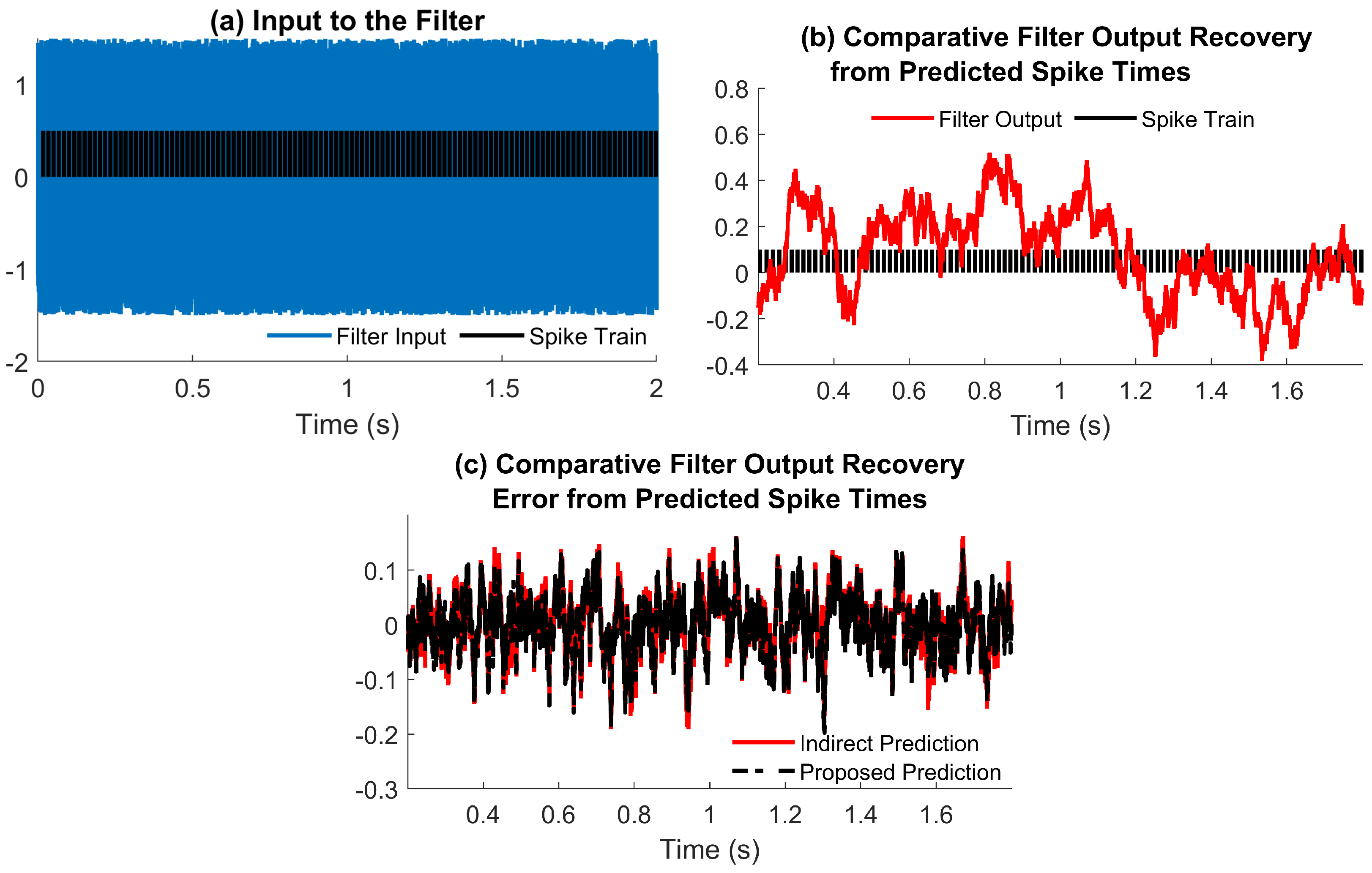
Theorem 1 shows that one can construct sequence t ˜ k , m y that approximates t k y with error 2 δ c b c 2 . We note that this error is dependent only on neuron parameters, and thus can be made arbitrarily small by changing the IF model. In practice, we use a finite sequence of input measurements t l u l = 0 , , L to approximate output samples t k y k = 0 , , K that satisfy t 0 u t k y t L u , k = 0 , , K . The proposed direct filtering method is summarized in Algorithm 1.
We note that, in practice, convergence was achieved in Algorithm 1 for M 4 iterations in all examples we evaluated. Moreover, we note that, in the proposed manuscript, computing t ˜ k + 1 y uses t ˜ k y as an initial condition. When new input data samples become available, Algorithm 1 incorporates them in computing new output data samples, but does not need to re-compute the output samples that are already known. In the next section, we numerically evaluate the proposed algorithm.
Algorithm 1 Computing the neuromorphic output data samples via the proposed method.
Data:  t k u , g ( t ) , δ , b;
Result:  t ˜ k y ;
Step 1. Set k = 1 and t ˜ 0 y = 0 . While t ˜ k 1 y < t L u ,
    Step 1a. t ˜ k , 0 y = t ˜ k 1 y ;
    Step 1b. Compute t ˜ k , m + 1 y = f ˜ k t ˜ k , m y for m = 1 , , M , where f ˜ k ( t ) = 1 b k δ Y ˜ t ,
Y ˜ t = l = 0 L U t l u G ( t t l u ) G ( t l u ) U t l u G ( t t l + 1 u ) + G ( t l + 1 u ) ,
    and G ( t ) = 0 t g ( τ ) d τ , U ( t l u ) = l δ b t l u , l = 0 , , L ;
    Step 1d. t ˜ k y = t ˜ k , M y ;
    Step 1e. k = k + 1 ;
Step 2. Set K = k 2 .

5. Numerical Study

In order to evaluate the performance of the proposed method, we define the following approximation errors:
  • Output inter-spike time error between the output of the time-encoded filter and the time-encoded output of the conventional filter:
    e j t ( k ) = t k + 1 y t k y t ˜ k + 1 y j t ˜ k y j , k = 1 , , K ,
    where t ˜ k y j is the output spike train prediction with Algorithm 1 ( j = 1 ) and the conventional method, involving the reconstruction of u ( t ) ( j = 2 ).
  • Output error between the decoded output of the time-encoded filter and the output of the conventional digital filter:
    e j y ( t ) = y ( t ) y ˜ j ( t ) , t [ 0 , 2 ] , j = 1 , 2 .
We compute the errors as percentages of true quantities t k + 1 y t k y and y ( t ) , respectively, by defining the following normalized error metrics:
ERR j t = 100 · e j t 2 k = 1 K t k + 1 y j t k y j 2 ( % ) , ERR j y = 100 · e j y L 2 y L 2 ( % ) .
Furthermore, we denote by Time 1 and Time 2 the computation times of the output spike train with the proposed and indirect methods, respectively. In our numerical examples, we discretize the time using a simulation time step of ε = 1 × 10 4 s . The parameters used, errors and computing times are summarized in Table 1.

5.1. Low-Pass Filtering of a Bandlimited Signal

The selected filter has the following transfer function:
G ( s ) = ω c s + ω c ,
where ω c = 10 rad / s . Furthermore, the input is generated as
u ( t ) = k = 1 N c k · sin ( Ω ( t k π / Ω ) ) Ω ( t k π / Ω ) , t 0 , 2 ,
where N = 191 and c k are random coefficients drawn from the uniform distribution on ( 1 , 1 ) , and Ω = 100 rad / 2 . We select c i = 0 , i 1 , 2 , 3 , N 2 , N 1 , N in order to avoid boundary errors for input recovery. The input and output of system G ( s ) are sampled with an integrate and fire neuron with parameters δ = 0.05 , b = 6 . Signals u ( t ) , y ( t ) and corresponding spike times are depicted in Figure 2a,b, respectively.
We estimate spike times t k y in two different ways, via the indirect method presented in Section 3 and the proposed direct method in Section 4. The results are depicted in Figure 3, and the recovery errors are ERR 1 t = 0.49 % for the proposed method and ERR 2 t = 0.75 % for the indirect method. Furthermore, the filter output errors are ERR 1 y = 0.82 % and ERR 2 y = 3.35 % . However, the computing times are 0.62 s for the proposed method and 2.93 s for the indirect method. We note that a major contribution in the error induced by the conventional method is due to boundary errors, which are a known artefact of reconstruction [12,33].

5.2. Low-Pass Filtering of Uniform White Noise

To show that the proposed method has no limitations in terms of input bandwidth, as indicated by the bounds in Theorem 1, here, we choose u ( t ) to be drawn from the random uniform distribution on [ 1.5 , 1.5 ] . Given that in this case, filter G ( s ) reduces significantly the noise amplitude, we amplify the output by 10 using the new filter, G ( s ) = 10 · ω c s + ω c , where ω c = 10 rad / s . The neuron parameters are δ = 0.1 , b = 6 . The input and output signals, as well as the output recovered with both methods, are presented in Figure 4a,b. The proposed prediction method does not need any knowledge of the input bandwidth. As an alternative, we reconstruct the input with the conventional indirect method, where the recovery bandwidth is Ω = 100 rad / s . The value of Ω is well above the cuttoff frequency of filter ω c , which leads to accurate recovery of the filter output. However, random input u ( t ) cannot be recovered for any Ω > 0 .
The output spike train prediction with both methods is presented in Figure 5a. The corresponding errors are ERR 1 t = 0.6 % , ERR 2 t = 1.06 % , ERR 1 y = 25.22 % , and ERR 2 y = 26.68 % , also summarized in Table 1. The computing times are 0.32 s for the proposed method and 0.81 s for the indirect method.

5.3. The Effect of Spike Density on Performance

During our experiments, we noticed that neuron threshold δ has an important role in deciding the computation time of both prediction routines. To illustrate this, we repeated the experiment in Section 5.2 using the same settings where δ was iteratively assigned 10 values uniformly spaced in interval [ 0.02 , 0.1 ] . As before, we measured the error on the predicted spike train, the reconstructed filter output and computation time for each method, illustrated in Figure 5b and Figure 6a,b, respectively.

5.4. Output Spike Prediction for Neuron Sampling below the Nyquist Rate

In the examples presented so far, the filter output is sampled at a rate that allows input reconstruction. In this example, we use a uniform white noise input bounded in [ 1.5 , 1.5 ] . The input is filtered using a bandpass filter computed employing the Daubechies orthogonal wavelet 30, depicted in Figure 7. We note that the effective bandwidth is around 1200 rad / s . When sampled with an IF with parameters δ = 0.04 , b = 6 , the filter output samples satisfy max t k + 1 y t k y = 0.0074 > π Ω = 0.0026 , which violates the condition for perfect recovery in (3). Therefore, in this example, we only evaluate the error using ERR j t , as ERR j y involves the reconstruction of the filter output from IF measurements.
We note that, as in Section 5.2 and Section 5.3, here, the input is not bandlimited, and its recovery cannot be guaranteed by (3). In this case, the choice of the bandwidth parameter Ω used in recovery is not determined by any existing theoretical result. We run the conventional method by changing the recovery bandwidth across 11 uniformly distributed values in interval 500 rad / s , 1500 rad / s . The comparative results are depicted in Figure 8a,b. We note that the proposed direct method does not have the bandwidth as a parameter, and therefore its performance is the same for all choices of Ω . The results show that the error introduced by the conventional method ERR 2 t changes quite significantly with Ω . An error around 15 % higher than the proposed method is achieved for Ω 600 , 1300 , but the difference becomes significantly larger for Ω outside this interval. Meanwhile, the computation time of the proposed method is more than one order of magnitude lower than that of the conventional method (see Figure 8b) for all values of Ω .

6. Conclusions

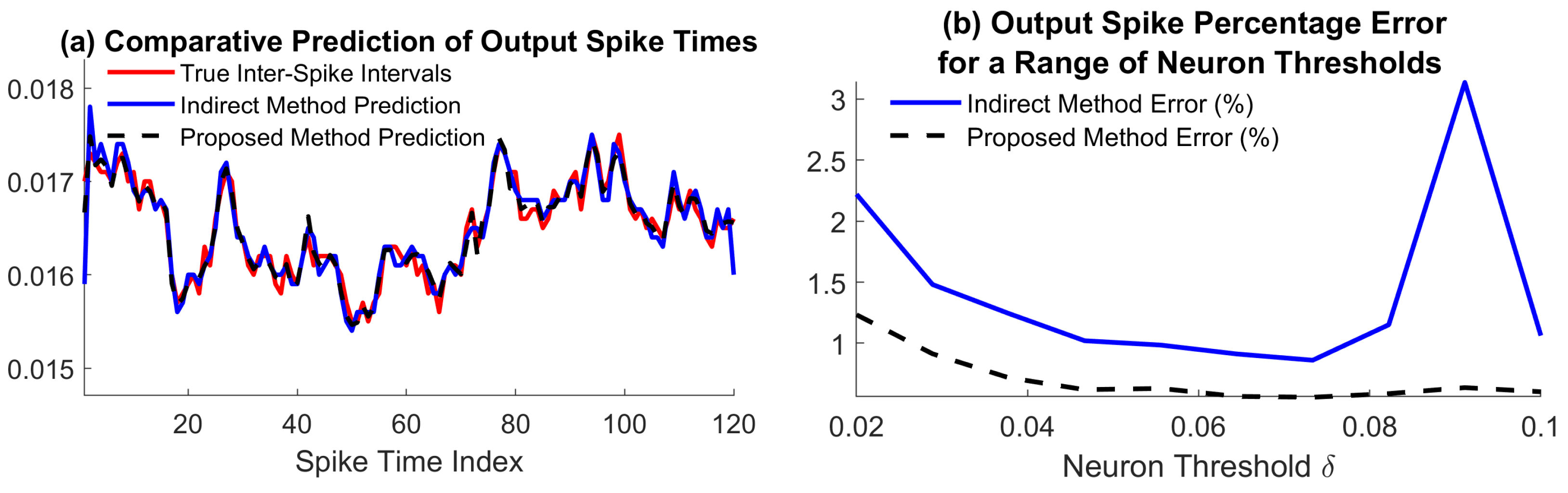
In this work, we introduced a new method to filter an analog signal via its neuromorphic measurements. Unlike existing approaches, the method does not require imposing smoothness type assumptions on the analog input and filter output, such as a limited bandwidth. We introduced recovery guarantees, showing that it is possible to approximate the output spike train with arbitrary accuracy for an appropriate choice of the sampling model. We compared the proposed method numerically against the conventional solution to this problem, which involves reconstruction of the analog signal. The results show the accuracy of the proposed method is comparable to that of the conventional approach. However, the computing time was smaller for the proposed method in all examples, ranging from 2–3 times up to more than one order of magnitude smaller.
Conceptually, the proposed method has the advantage of not depending on the characteristics of the analog signal, and therefore it is not restricted to satisfy any reconstruction guarantees. As demonstrated numerically, the method works well in the case of random inputs, as well as when the input and output of the filter are sampled below Nyquist. Moreover, given the fact that it bypasses input reconstruction, the proposed method is not affected by known artefacts of recovery methods such as boundary errors.
This work can be extended in several directions. First, the theoretical results can be extended to work with higher-order interpolation rather than a piecewise constant, which may lead to better error bounds. Second, the results can be extended for the more general scenarios of multichannel or nonlinear filters. Third, the proposed algorithm could be implemented in hardware and tested in practical communication scenarios. This work has the potential to lead to the development of neuromorphic filters that would facilitate a faster transition towards a power-efficient computing infrastructure.

Author Contributions

All the authors have contributed substantially to the paper. D.F. conceptualized the methodology, performed numerical studies and prepared the draft paper. D.C. contributed in the writing phase through review and editing. All authors have read and agreed to the published version of the manuscript.

Funding

This research received no external funding. The APC is funded by the Imperial College London Open Access Fund.

Data Availability Statement

Data is contained within the article.

Conflicts of Interest

The authors declare no conflict of interest.

Abbreviations

The following abbreviations are used in this manuscript:
IFIntegrate and fire
TEMTime encoding machine

References

  1. Rabiner, L.R.; Gold, B. Theory and Application of Digital Signal Processing; Prentice-Hall: Englewood Cliffs, NJ, USA, 1975. [Google Scholar]
  2. Lazar, A.A.; Tóth, L.T. Perfect recovery and sensitivity analysis of time encoded bandlimited signals. IEEE Trans. Circuits Syst. I 2004, 51, 2060–2073. [Google Scholar] [CrossRef]
  3. Roza, E. Analog-to-digital conversion via duty-cycle modulation. IEEE Trans. Circuits Syst. II 1997, 44, 907–914. [Google Scholar] [CrossRef]
  4. Chen, J.; Skatchkovsky, N.; Simeone, O. Neuromorphic integrated sensing and communications. IEEE Wirel. Commun. Lett. 2022, 12, 476–480. [Google Scholar] [CrossRef]
  5. Skatchkovsky, N.; Jang, H.; Simeone, O. Spiking neural networks—Part III: Neuromorphic communications. IEEE Commun. Lett. 2021, 25, 1746–1750. [Google Scholar] [CrossRef]
  6. Abdul-Kreem, L.I.; Neumann, H. Estimating visual motion using an event-based artificial retina. In Computer Vision, Imaging and Computer Graphics Theory and Applications, Proceedingsofthe 10th International Joint Conference, VISIGRAPP 2015, Berlin, Germany, 11–14 March 2015; Revised Selected Papers 10; Springer: Cham, Switzerland, 2016; pp. 396–415. [Google Scholar]
  7. Gallego, G.; Delbrück, T.; Orchard, G.; Bartolozzi, C.; Taba, B.; Censi, A.; Leutenegger, S.; Davison, A.J.; Conradt, J.; Daniilidis, K.; et al. Event-based vision: A survey. IEEE Trans. Pattern Anal. Mach. Intell. 2020, 44, 154–180. [Google Scholar] [CrossRef] [PubMed]
  8. Kowalczyk, M.; Kryjak, T. Interpolation-Based Event Visual Data Filtering Algorithms. In Proceedings of the IEEE/CVF Conference on Computer Vision and Pattern Recognition, Vancouver, BC, Canada, 17–24 June 2023; pp. 4055–4063. [Google Scholar]
  9. Scheerlinck, C.; Barnes, N.; Mahony, R. Asynchronous spatial image convolutions for event cameras. IEEE Robot. Autom. Lett. 2019, 4, 816–822. [Google Scholar] [CrossRef]
  10. Lazar, A.A. A simple model of spike processing. Neurocomputing 2006, 69, 1081–1085. [Google Scholar] [CrossRef]
  11. Florescu, D.; Coca, D. Implementation of linear filters in the spike domain. In Proceedings of the 2015 European Control Conference (ECC), Linz, Austria, 15–17 July 2015; pp. 2298–2302. [Google Scholar]
  12. Lazar, A.A. Time encoding with an integrate-and-fire neuron with a refractory period. Neurocomputing 2004, 58, 53–58. [Google Scholar] [CrossRef]
  13. Florescu, D.; Coca, D. A novel reconstruction framework for time-encoded signals with integrate-and-fire neurons. Neural Comput. 2015, 27, 1872–1898. [Google Scholar] [CrossRef]
  14. Paninski, L.; Pillow, J.W.; Simoncelli, E.P. Maximum likelihood estimation of a stochastic integrate-and-fire neural encoding model. Neural Comput. 2004, 16, 2533–2561. [Google Scholar] [CrossRef]
  15. Florescu, D.; Coca, D. Identification of linear and nonlinear sensory processing circuits from spiking neuron data. Neural Comput. 2018, 30, 670–707. [Google Scholar] [CrossRef]
  16. Maass, W.; Natschläger, T.; Markram, H. Real-time computing without stable states: A new framework for neural computation based on perturbations. Neural Comput. 2002, 14, 2531–2560. [Google Scholar] [CrossRef]
  17. Florescu, D.; Coca, D. Learning with precise spike times: A new decoding algorithm for liquid state machines. Neural Comput. 2019, 31, 1825–1852. [Google Scholar] [CrossRef] [PubMed]
  18. Florescu, D. A Generalized Approach for Recovering Time Encoded Signals with Finite Rate of Innovation. arXiv 2023, arXiv:2309.10223. [Google Scholar]
  19. Gontier, D.; Vetterli, M. Sampling based on timing: Time encoding machines on shift-invariant subspaces. Appl. Comput. Harmon. Anal. 2014, 36, 63–78. [Google Scholar] [CrossRef]
  20. Alexandru, R.; Dragotti, P.L. Reconstructing classes of non-bandlimited signals from time encoded information. IEEE Trans. Signal Process. 2019, 68, 747–763. [Google Scholar] [CrossRef]
  21. Hilton, M.; Dragotti, P.L. Sparse Asynchronous Samples from Networks of TEMs for Reconstruction of Classes of Non-Bandlimited Signals. In Proceedings of the IEEE International Conference on Acoustics, Speech and Signal Processing (ICASSP), Rhodes Island, Greece, 4–10 June 2023. [Google Scholar]
  22. Lazar, A.A.; Pnevmatikakis, E.A. Faithful representation of stimuli with a population of integrate-and-fire neurons. Neural Comput. 2008, 20, 2715–2744. [Google Scholar] [CrossRef] [PubMed]
  23. Shannon, C.E. Communication in the presence of noise. Proc. IRE 1949, 37, 10–21. [Google Scholar] [CrossRef]
  24. Feichtinger, H.G.; Gröchenig, K. Theory and practice of irregular sampling. Wavelets Math. Appl. 1994, 305–363. [Google Scholar]
  25. Gröchenig, K. Reconstruction algorithms in irregular sampling. Math. Comput. 1992, 59, 181–194. [Google Scholar] [CrossRef]
  26. Aldroubi, A.; Gröchenig, K. Nonuniform sampling and reconstruction in shift-invariant spaces. SIAM Rev. 2001, 43, 585–620. [Google Scholar] [CrossRef]
  27. Christensen, O. An Introduction to Frames and Riesz Bases; Birkhauser: Boston, NJ, USA, 2003. [Google Scholar]
  28. Lazar, A.A.; Pnevmatikakis, E.A. Consistent Recovery of Sensory Stimuli Encoded with MIMO Neural Circuits. Comput. Intell. Neurosci. 2010, 2010, 469658. [Google Scholar] [CrossRef] [PubMed]
  29. Lazar, A.A.; Pnevmatikakis, E.A. Reconstruction of sensory stimuli encoded with integrate-and-fire neurons with random thresholds. EURASIP J. Adv. Signal Process. 2009, 2009, 682930. [Google Scholar] [CrossRef] [PubMed]
  30. Lazar, A.A.; Slutskiy, Y.B. Channel identification machines. Comput. Intell. Neurosci. 2012, 2012, 209590. [Google Scholar] [CrossRef] [PubMed]
  31. Lazar, A.A.; Zhou, Y. Identifying multisensory dendritic stimulus processors. IEEE Trans. Mol. Biol. Multi-Scale Commun. 2016, 2, 183–198. [Google Scholar] [CrossRef]
  32. Lazar, A.A.; Zhou, Y. Volterra dendritic stimulus processors and biophysical spike generators with intrinsic noise sources. Front. Comput. Neurosci. 2014, 8, 95. [Google Scholar] [CrossRef]
  33. Lazar, A.A.; Simonyi, E.K.; Tóth, L.T. An overcomplete stitching algorithm for time decoding machines. IEEE Trans. Circuits Syst. I 2008, 55, 2619–2630. [Google Scholar] [CrossRef]
Figure 1. Approximating the output of an analog filter using input measurements. In the case of uniform sampling measurements (bottom), digital filters are well known and have been studied exhaustively. Mapping the filter input to the output was not studied extensively for neuromorphic measurements. The conventional approach is to reconstruct the input and compute filtering in the analog domain, which is time consuming and not always possible.
Jlpea 13 00063 g001
Figure 2. Output spike train prediciton for a bandlimited input. (a) Filter input and the corresponding spike train. (b) Filter output and the corresponding spike train. (c) Recovery errors e 2 y ( t ) and e 1 y ( t ) with the indirect and proposed method, respectively.
Jlpea 13 00063 g002
Figure 3. Spike train prediction comparative performance: the true inter-spike intervals, interposed on the predicted inter-spike intervals with the indirect and proposed methods, respectively.
Jlpea 13 00063 g003
Figure 4. Output spike train prediction for uniform random noise. (a) Filter input and corresponding spike train. (b) Filter output and corresponding spike train. (c) Recovery errors e 2 y ( t ) and e 1 y ( t ) with the indirect and proposed methods, respectively.
Jlpea 13 00063 g004
Figure 5. (a) Spike train prediction comparative performance: the true inter-spike intervals, interposed on the predicted inter-spike intervals with the indirect and proposed methods, respectively. (b) Spike train prediction comparative performance for 10 values of δ uniformly spaced in [ 0.02 , 0.1 ] .
Jlpea 13 00063 g005
Figure 6. Filter output computation for 10 values of δ uniformly spaced in [ 0.02 , 0.1 ] . (a) Analog output error. (b) Computation time.
Jlpea 13 00063 g006
Figure 7. Bandpass filter computed via the Daubechies orthogonal wavelet 30.
Jlpea 13 00063 g007
Figure 8. Filter output computation for 11 values of the reconstruction bandwidth uniformly spaced in [ 500 rad / s , 1500 rad / s ] . (a) Spike train output error. (b) Computation time.
Jlpea 13 00063 g008
Table 1. The parameters used in our numerical simulations section are summarized below.
ExampleInputFilter δ ERR 1 t (%) ERR 2 t (%) ERR 1 y (%) ERR 2 y (%) Time 1 (s) Time 2 (s)
5.1Low passLow pass 0.05 0.49 0.75 0.82 3.35 0.62 2.93
5.2Uniform NoiseLow pass 0.1 0.6 1.06 25.2 26.6 0.32 0.81
5.3Uniform NoiseLow pass0–0.10.5–1.31–322–2524–320.1–11–20
5.4Uniform NoiseWavelet 0.04 2.85 3.2 N/AN/A 0.2 3
Disclaimer/Publisher’s Note: The statements, opinions and data contained in all publications are solely those of the individual author(s) and contributor(s) and not of MDPI and/or the editor(s). MDPI and/or the editor(s) disclaim responsibility for any injury to people or property resulting from any ideas, methods, instructions or products referred to in the content.

