Reinforcement Learning-Based Multi-Objective Optimization for Generation Scheduling in Power Systems

Abstract

Multi-objective power scheduling (MOPS) aims to address the simultaneous minimization of economic costs and different types of environmental emissions during electricity generation. Recognizing it as an NP-hard problem, this article proposes a novel multi-agent deep reinforcement learning (MADRL)-based optimization algorithm. Within a custom multi-agent simulation environment, representing power-generating units as collaborative types of reinforcement learning (RL) agents, the MOPS problem is decomposed into sequential Markov decision processes (MDPs). The MDPs are then utilized for training an MADRL model, which subsequently offers the optimal solution to the optimization problem. The practical viability of the proposed method is evaluated across several experimental test systems consisting of up to 100 units featuring bi-objective and tri-objective problems. The results demonstrate that the proposed MADRL algorithm has better performance compared to established methods, such as teaching learning-based optimization (TLBO), real coded grey wolf optimization (RCGWO), evolutionary algorithm based on decomposition (EAD), non-dominated sorting algorithm II (NSGA-II), and non-dominated sorting algorithm III (NSGA-III).

1. Introduction

Due to the instantaneous nature of electrical power and its inability to be stored in massive quantities, its demand exhibits temporal fluctuations. This dynamic nature of electrical consumption prompts the need for reliable power scheduling [1]. Central to power scheduling is the fundamental requirement that the power supply match the demand at each period of a particular planning horizon. Power system operators utilize a set of generating units to achieve this equilibrium, each with its own technological and operational constraints. The cost of power generation also varies among generating units, and it is not directly proportional to the power output [2]. Economic cost dispatch (ECD) forms the foundational aspect of power scheduling, representing a single-objective optimization problem. Subject to various unit-specific and system-level constraints, ECD determines the optimal loads of generating units that minimize the operating costs. This process requires a delicate balance among fluctuating demands, operational constraints, and economic considerations. There are also growing concerns about the environmental impact of power generation because approximately two-thirds of electric energy is currently derived from fossil fuels [3]. Fossil fuels are the major contributors to greenhouse gases (GHGs) and other pollutants such as carbon dioxide (CO₂), nitrous oxide (NO_x), and sulfur dioxide (SO₂). The power scheduling problem has, thus, expanded to a multi-objective optimization problem, encompassing environmental emission dispatch (EED). As a result, multi-objective power scheduling (MOPS) seeks to find an optimal dispatch schedule that minimizes both economic costs and several types of environmental emissions.

MOPS is an intricate optimization problem characterized by several complex factors. First, it involves a combinatorial dimensionality explosion, which makes it extraordinarily difficult as the number of generating units increases [4,5]. Each generating unit’s unique characteristics and constraints add another layer of intricacy [6,7]. Ramp rate constraints additionally complicate the decision-making process since they contribute to the non-smooth and discontinuous nature of the input–output characteristics of generating units [8,9,10]. Valve point effects (VPEs) are other factors affecting the input–output characteristics of thermal generating units. Incorporating VPEs into the scheduling problem thereby intensifies the complexities of power scheduling. Furthermore, real-world power systems require multi-period planning to adapt to changing demand patterns and resource availability. Since multi-period planning duplicates the constraints for each period, it compounds the exponential escalation of dimensionality [4,5,11]. Current global environmental policies, such as the Sustainable Development Goals (SDGs), emphasize the reduction of greenhouse gases (GHGs) through integrating renewable energy sources into power networks [12]. While renewables offer environmental benefits, their intermittent nature and weather dependence may lead to significant power supply fluctuations [13]. Additionally, uncertainties in real-world scenarios, including unit and transmission line outages, may complicate power system management even more. Therefore, the MOPS problem poses a multifaceted challenge due to its high dimensionality, multiple constraints spanning multiple periods, non-smooth and non-convex characteristics, and inherent uncertainties.

The MOPS problem has drawn much attention to the development of various optimization models. The methodologies can be grouped into mathematical models, meta-heuristic approaches, and hybrid methods. Mathematical models include priority list (PL), dynamic programming (DP), Lagrangian relaxation (LR), mixed integer linear programming (MILP) [14], and mixed integer quadratic programming (MIQP) [5]. Many of these models are grounded in heuristic principles [4,5]. The ability of these models to guarantee optimal solutions is limited [11], and they face computational inefficiencies, particularly when tackling larger-scale power scheduling problems [15]. Specifically, the PL method is susceptible to poor solution quality [16,17], while DP, MILP, and MIQP encounter dimensionality problems [16,17]. Some specific models also exhibit shortcomings in handling specific constraints, potentially leading to system instability [18]. Moreover, these models are rooted in heuristic principles [4,5], and their ability to guarantee optimal solutions is limited [11]. They also grapple with numerical convergence issues [19]. While effective for scheduling problems with lower dimensions and fewer constraints [20], applying these model-based methods to a more complex scenario raises concerns. Meta-heuristic techniques have been introduced as a promising alternative to address the limitations of mathematical methods. These approaches amalgamate fundamental heuristic principles to enhance the exploration and exploitation of potentially feasible solutions. The most common metaheuristic methods used for power scheduling are differential evolution (DE) [21], genetic algorithms (GA) [22], teaching learning-based optimization (TLBO) [23,24], binary-real-coded genetic algorithm (BRCGA) [25], binary alternative moth-flame optimization (BAMFO) [18], binary bat search algorithm (BBSA) [26], new binary particle swarm optimization (NBPSO) [20], improved dragonfly algorithm particle swarm optimization (iDA-PSO) [27], binary particle swarm optimization (BPSO) [20], quantum-inspired evolutionary algorithm (QEA) [28], quantum evolutionary programming (QEP) [16], quantum inspired binary grey wolf optimizer (QI-BIGWO) [16], quasi-oppositional teaching learning-based algorithm (QOTLBO) [24], binary grey wolf optimizer (BGWO) [29], binary learning particle swarm optimization (BLPSO) [20], binary moth-flame optimization (BMFO) [18], binary coded modified moth flame optimization algorithm (BMMFOA) [30], and teaching learning-based optimization (TLBO) [24]. A comprehensive review of metaheuristic optimization algorithms is provided by [31]. The third category is to use hybrid approaches that combine mathematical and heuristic strategies. The whale optimization algorithm (WOA) [32], the particle swarm optimization (PSO) [33], the grey wolf optimization (GWO) [28,34], the non-dominated sorting genetic algorithm-II (NSGA-II) [35], the non-dominated sorting genetic algorithm-III (NSGA-III) [36], and the evolutionary algorithm based on decomposition (EAD) [37] are some well-known examples applied for power scheduling. Even though these methods integrate diverse strategies, they are still heuristic, and there is no guarantee that they can find global optima [31].

Despite the availability of various optimization techniques, solving MOPS remains an NP-hard (non-deterministic polynomial-time hard) problem [7]. In their attempts to simplify the complexity, many existing studies have tended to overlook the holistic perspective of power scheduling [15]. For instance, several studies [34,38,39] have delved into single-objective power scheduling (SOPS), primarily focusing on minimizing economic costs. While power scheduling is multi-objective, the narrow focus on financial costs might lead to higher emissions, pose health risks, and contribute to climate change and global warming. Furthermore, the studies often involve a limited number of generating units and constraints [40]. Most existing approaches have also focused on single-period problems, simplifying multi-period constraints. Such simplification disregards the broader dynamics and uncertainties that may influence power generation and consumption over a longer planning horizon. Studies like [23,41] have investigated systems with up to 100 units. However, they have overlooked ramp rate constraints and thermal valve point effects (VPEs), which are critical for accurate modeling [8,11]. This means the studies have failed to account for the non-smooth and non-convex nature of the cost and emission functions [8,9,34]. Moreover, effective operational schedules should grapple with power system uncertainties that intermittent renewable energy sources, sudden demand fluctuations, unit outages, and transmission losses may cause. However, many existing optimization models have overlooked these critical aspects of power scheduling [1], potentially leading to suboptimal solutions. These oversights underscore the necessity for a more comprehensive and nuanced approach to addressing the complexities of MOPS.

Due to recent advancements in artificial intelligence (AI), the landscape of decision-making approaches has undergone a paradigm shift. Specifically, reinforcement learning (RL) has emerged as a potent tool for making intelligent decisions in dynamically changing environments [40]. RL, being model-free, is particularly suitable for simulating uncertain real-world scenarios that lack accurate mathematical formulations [29,42]. Its trial-and-error-based approach and inherent adaptability make it a powerful method for handling stochasticity [43]. Despite this potential, RL-based methods are underutilized in power scheduling [42], as shown in Table 1.

Two main RL-based approaches are utilized in the literature for power scheduling: tabular Q-learning [43,44] and function approximation-based Q-learning [5,12,29,40,42,45,46]. The initial tabular Q-learning has been demonstrated in [43], where the pursuit exploration method has been used to examine a four-unit power scheduling problem. Another study utilized tabular Q-learning to solve a three-unit problem. It is reported that Q-learning performed better than the conventional PL method [44]. On the other hand, the function approximation-based Q-learning approach yielded improved solutions over simulated annealing (SA) [47], despite their small-scale experiment involving only eight units. The adoption of the MDP framework in an RL-based approach by [12] was also instrumental in achieving superior outcomes. Furthermore, a centralized Q-learning-based optimization algorithm was compared with a distributed counterpart [29]. Fuzzy Q-learning also outperformed GWO in its application in handling a power system with 10 generators [45]. An adaptive multi-step Q-learning algorithm was employed for a five-unit power system [5], surpassing MIQP. It can be observed that Q-learning methods implemented thus far have primarily been confined to small power systems consisting of 3 to 10 units. This limitation arises from the challenges posed by extensive state and action spaces due to the inherently combinatorial nature of the problem. The studies by [40,46] have addressed up to 30-unit power systems and reported better performance than MILP. Though up to 100 units are implemented by [42] and the solutions are better than GA, the study compromised ramp rate constraints and VPEs.

Table 1. Summary of RL-based power scheduling studies.

Reference	Objective	Units	Constraints				VPEs
			Production Capacity	Operating Duration	Ramp Rates	Reserve
[43]	Single	4	Yes	No	No	No	No
[44]	Single	3	Yes	No	No	No	No
[47]	Single	8	Yes	Yes	No	No	No
[12]	Single	10	Yes	Yes	No	No	No
[45]	Single	10	Yes	Yes	Yes	Yes	No
[29]	Single	$\le$10	Yes	No	No	No	Yes
[5]	Single	5	Yes	Yes	Yes	No	No
[40]	Single	$\le$30	Yes	Yes	No	No	No
[46]	Single	$\le$30	Yes	Yes	No	No	No
[42]	Single	$\le$100	Yes	Yes	No	Yes	No

Table 1. Summary of RL-based power scheduling studies.

Reference	Objective	Units	Constraints				VPEs
			Production Capacity	Operating Duration	Ramp Rates	Reserve
[43]	Single	4	Yes	No	No	No	No
[44]	Single	3	Yes	No	No	No	No
[47]	Single	8	Yes	Yes	No	No	No
[12]	Single	10	Yes	Yes	No	No	No
[45]	Single	10	Yes	Yes	Yes	Yes	No
[29]	Single	$\le$10	Yes	No	No	No	Yes
[5]	Single	5	Yes	Yes	Yes	No	No
[40]	Single	$\le$30	Yes	Yes	No	No	No
[46]	Single	$\le$30	Yes	Yes	No	No	No
[42]	Single	$\le$100	Yes	Yes	No	Yes	No

Generally, the existing RL-based studies have demonstrated their superiority over traditional methods such as PL, SA, LR, MILP, MIQP, GWO, and GA. However, most of these achievements have been confined to smaller-scale problems. Additionally, most RL models have neglected to ensure reserve capacity to handle unforeseen circumstances like sudden spikes in demand, generating unit failures, or transmission line losses. Further, the impact of ramp rate constraints and VPEs has frequently been omitted from consideration in the models. It is also noted that the previous studies focused on the single-objective problem of minimizing economic costs. Thus, the existing studies inadvertently neglected the crucial aspect of the environmental impact of carbon emissions. More specifically, no known RL-based method has been applied to MOPS problems. Solutions derived from simplified power scheduling problems may not accurately capture the complexities of real-world power systems [42].

These existing disparities underscore a significant research gap that emphasizes the pressing need to develop a scalable RL algorithm that could potentially unlock innovative solutions and pave the way for more effective and reliable power scheduling techniques without compromising the characteristics of a realistic power system. This study introduces an innovative MOPS optimization approach based on multi-agent reinforcement learning. The proposed method utilizes a contextually adaptive multi-agent simulation environment where power-generating units are represented as agents. The dynamics of MOPS are simulated within this environment using Markov decision processes (MDPs), which are then used to train a multi-agent deep RL (MADRL) model. The solution for the optimization problem is derived from the trained MADRL model.

In summary, the contributions of this article are as follows:

• The primary contribution is the introduction of a pioneering MADRL-based optimization algorithm that can solve single- to tri-objective power scheduling problems. The algorithm harnesses the power of MADRL to decisively confront the intricate challenges of MOPS.
• Unlike existing methods, the proposed algorithm does not confine itself to a limited planning horizon and a fixed number of generating units. It also encompasses a comprehensive set of unit-specific (including ramp rates and VPEs) and system-level constraints such as reserve availability.
• Another distinctive contribution to our approach is developing a contextually adaptive multi-agent simulation environment. The environment is used to decompose the MOPS problem into sequential MDPs. It can contextually correct agents’ illegal decisions and adjust excess and shortages of supply capacities. By accelerating agents’ learning and reducing model training time, the simulation environment may significantly enhance the efficiency of the entire optimization process.
• The simulation environment is not specifically tailored to train a specific RL model but is model agnostic. This adaptability allows researchers and practitioners to train and explore diverse types of RL models for solving power scheduling.
• Unlike traditional models with exponential dimensionality (i.e., $\mathcal{O}\left(2^n\right)$ for $n$ generating units), the proposed algorithm has linear dimensionality (i.e., $\mathcal{O}\left(2n\right)$). This characteristic underscores its scalability and better performance to handle large-scale problems compared to existing methods.
• The algorithm’s programming code has been verified by Code Ocean for quality and computational reproducibility (https://doi.org/10.24433/CO.9235622.v1) and published as an open-source software package [48]. This initiative may facilitate results replication and foster a spirit of experimentation and further extensions within the research community.

The remainder of this article is organized as follows: Section 2 describes the description and formulation of the MOPS objective problem. Section 3 briefly outlines the procedural framework of the proposed optimization methodology. Section 4 presents practical applications and results, and Section 5 presents the concluding remarks.

2. MOPS Problem Formulation

Consider a power scheduling problem consisting of $n$ thermal generating units, all subject to optimization, over a planning horizon with $T$ periods. Given operating durations $({\mathcal{t}}_{ti}\in \mathbb{R};\forall i$) at each period $t$, two decision variables are associated with each unit. The first is a unit commitment (UC), indicating whether a unit is committed $\left({\mathcal{t}}_{ti}>0\right)$ or not $\left({\mathcal{t}}_{ti}<0\right)$, and the second is the power output $\left(p_{ti},\forall t,i\right)$.

2.1. Cost Objective Function

The operating cost ($/period) of each unit $i$ during each period $t$ encompasses three components: production cost ${\mathcal{C}}^{on}\left(p_{ti}\right)$, startup cost ${\mathcal{C}}_{ti}^{su}$, and shutdown cost $c_{ti}^{sd}$ [49]. Considering operating durations and transitions between online and offline statuses, its comprehensive computation is specified as follows:

$${\mathcal{C}}_{ti}=⟦{\mathcal{t}}_{ti}>0⟧{\mathcal{C}}^{on}\left(p_{ti}\right)+⟦{\mathcal{t}}_{ti}>0⟧⟦{\mathcal{t}}_{t-1,i}<0⟧{\mathcal{C}}_{ti}^{su}+⟦{\mathcal{t}}_{ti}<0⟧⟦{\mathcal{t}}_{t-1,i}>0⟧{\mathcal{C}}_{ti}^{sd};\forall t,i.$$

(1)

The production cost ${\mathcal{C}}^{on}\left(p_{ti}\right)$ is typically represented by a quadratic function of the power output $p_{ti}$. Unlike the usual model-based optimization methods, the proposed MADRL approach does not necessitate approximating production costs with smooth and convex functions that disregard VPEs. Consequently, the production cost function incorporates a sinusoidal term to account for VPEs [50], which can be written as follows:

$${\mathcal{C}}^{on}\left(p_{ti}\right)={\alpha }_i^c{p}_{ti}^2+{\beta }_i^c{p}_{ti}+{\delta }_i^c+|{\rho }_i^c\mathrm{s}\mathrm{i}\mathrm{n}[{\phi }_i^c(p_i^{min}-p_{ti})\left]\right|;\forall t,i.$$

(2)

The objective of ECD is to minimize the total operating costs over the entire planning horizon, defined as follows:

$$\mathcal{C}=\sum _{t=1}^T{\mathcal{C}}_t=\sum _{t=1}^T\sum _{i=1}^n{\mathcal{C}}_{ti}.$$

(3)

2.2. Emission Objective Function

As mentioned earlier, electricity generation is the major contributor to GHGs and environmental pollutants. Specifically, the combustion of carbon-containing fossil fuels, such as coal, oil, or natural gas, results in the production of CO₂. CO₂ is a major contributor to climate change and/or global warming. The combustion of fuels containing sulfur compounds also releases SO₂. SO₂ is a precursor to acid rain and can have detrimental effects on the quality of the air. Consequently, beyond the economic implications, addressing environmental emissions becomes crucial to mitigating the impacts of global warming and air pollution.

Similar to the costs associated with power generation, emissions are not directly tied to power outputs and exhibit variations among different generating units. Mathematically, the operating emissions (lbs/hour) for each unit $i$ during each period $t$ are the sum of startup ${\mathcal{E}}_{ti}^{su}$, shutdown ${\mathcal{E}}_{ti}^{sd}$, and production ${\mathcal{E}}^{on}\left(p_{ti}\right)$ emissions.

$${\mathcal{E}}_{ti}=⟦{\mathcal{t}}_{ti}>0⟧{\mathcal{E}}^{on}\left(p_{ti}\right)+⟦{\mathcal{t}}_{ti}>0⟧⟦{\mathcal{t}}_{t-1,i}<0⟧{\mathcal{E}}_{ti}^{su}+⟦{\mathcal{t}}_{ti}<0⟧⟦{\mathcal{t}}_{t-1,i}>0⟧{\mathcal{E}}_{ti}^{sd};\forall t,i$$

(4)

Like the production cost functions, non-smooth and non-convex functions are used for the production emissions, which are expressed as follows:

$${\mathcal{E}}^{on}\left(p_{ti}\right)={\alpha }_i^e{p}_{ti}^2+{\beta }_i^e{p}_{ti}+{\delta }_i^e+{\rho }_i^{\mathrm{e}}\exp \left({\phi }_i^e{p}_{ti}\right);\forall t,i.$$

(5)

The total daily emissions over the entire planning horizon can then be consolidated as follows:

$$\mathcal{E}=\sum _{t=1}^T{\mathcal{E}}_t=\sum _{t=1}^T\sum _{i=1}^n{\mathcal{E}}_{ti}.$$

(6)

The costs and emissions linked to generating units exhibit an inherent conflict [51]. Hence, operating at minimum cost alone (i.e., Equation (3)) or at absolute emission level (i.e., Equation (6)) is no longer acceptable because minimizing one leads to an increase in the other.

2.3. MOPS Objective Function

The objective function for MOPS is usually formulated by combining the separate cost and emission functions in Equations (3) and (6), respectively, into one. Traditionally, various methods have been widely employed, such as emission constraints, weighted-sum approaches, and cost-penalty factors. However, these methods come with inherent limitations. Emission constraints often fall short of adapting to real-time changes and tend to prioritize compliance over effective emission reduction strategies [42]. The weighted-sum approach faces challenges in striking the right trade-offs between costs and emissions [31]. The specific value of the weight might have an insignificant impact when costs and emissions are quite different in size [52]. It also exhibits limited efficiency for non-convex Pareto-optimal fronts [53] and applies only to convex cost and emission functions [54]. The cost-penalty method is used to convert emission curves into equivalent cost curves. However, its application is limited to increasing cost and emission functions. Additionally, its estimates are often unrealistically small or large. Consequently, this approach fails to capture the intricate relationships among the components [29]. Merging conflicting objectives may further obscure the trade-off relationship between cost and emissions, resulting in suboptimal solutions that do not fully exploit the potential for minimizing costs and emissions independently. This hindrance makes identifying Pareto-optimal solutions representing the best compromises between conflicting objectives challenging. In addressing these challenges, this study proposes a new hybrid approach to formulating the objective function. First, the production cost function in Equation (2) and the production emission function in Equation (5) are unified using both weight hyperparameters and unit-specific cost-to-emission conversion parameters, as follows:

$${\mathsf{\Phi }}^{on}\left(p_{t1},p_{t2}\dots ,p_{tn}\right)=\omega \sum _{i=1}^n⟦{\mathcal{t}}_{ti}>0⟧{\mathcal{C}}_{ti}^{on}\left(p_{ti}\right)+\left(1-\omega \right)\sum _{i=1}^n⟦{\mathcal{t}}_{ti}>0⟧{\eta }_i{\mathcal{E}}_{ti}^{on}\left(p_{ti}\right)$$

(7)

where $\omega$ and ${\eta }_i$ denote the weight hyperparameter ($0<\omega <1)$ and the cost-to-emission conversion parameter (${\eta }_i>0$), respectively. Equation (7) represents a bi-objective power scheduling problem, holding economic costs on one side and emissions on the other side. Considering $m$ types of environmental emissions, it can be extended to a general MOPS problem, and written as follows:

$${\Phi }^{on}\left(p_{t1},p_{t2}\dots ,p_{tn}\right)=\sum _{i=1}^n\left[⟦{\mathcal{t}}_{ti}>0⟧{\omega }_0{\mathcal{C}}_{ti}^{on}\left(p_{ti}\right)+\sum _{k=1}^m⟦{\mathcal{t}}_{ti}>0⟧{\omega }_k{\eta }_{ik}{\mathcal{E}}_{tik}^{on}\left(p_{ti}\right)\right]$$

(8)

where ${\omega }_k$ represents the weight associated with objective $k$ such that ${\omega }_k\ge 0$ and $\sum _{k=0}^m{\omega }_k=1$. The parameter ${\eta }_{ik}$ is the cost-to-emission conversion factor for unit $i$ corresponding to emission type $k$. This formulation not only allows the representation of emissions as continuous variables but also maintains their relative importance within the integrated production function.

Second, the startup and shutdown costs and emissions are aggregated separately. Consequently, the objective function of the MOPS consists of three separate components, which can be expressed as follows:

$$\Phi =\left[\sum _{t=1}^T{\Phi }^{on}\left(p_{t1},p_{t2}\dots ,p_{tn}\right), \sum _{t=1}^T{\mathcal{C}}_t^{su,sd}, \sum _{t=1}^T{\mathcal{E}}_t^{su,sd}\right]$$

(9)

where ${\mathcal{C}}_t^{su,sd}=\sum _{i=1}^n⟦{\mathcal{t}}_{ti}>0⟧\left(1-⟦{\mathcal{t}}_{t-1,i}<0⟧\right){\mathcal{C}}_{ti}^{su}+\left(1-⟦{\mathcal{t}}_{ti}>0⟧\right)⟦{\mathcal{t}}_{t-1,i}<0⟧{\mathcal{C}}_{ti}^{sd};\forall t$ and ${\mathcal{E}}_t^{su,sd}=\sum _{i=1}^n⟦{\mathcal{t}}_{ti}>0⟧\left(1-⟦{\mathcal{t}}_{t-1,i}<0⟧\right){\mathcal{E}}_{ti}^{su}+\left(1-⟦{\mathcal{t}}_{ti}>0⟧\right)⟦{\mathcal{t}}_{t-1,i}<0⟧{\mathcal{E}}_{ti}^{sd};\forall t$.

In contrast to existing approaches, the objective function in Equation (9) is not intrinsically converted to a single-objective function. Rather, it consists of three components: the transformed production value, the cost of startup and shutdown, and the emissions during startup and shutdown. This innovative formulation is designed to tackle the limitations of traditional methods, offering a more resilient and flexible solution to the simultaneous optimization of cost and emissions. For the sake of simplicity, let us denote each objective by ${\mathcal{O}}_k\left(k=\mathrm{0,1},..m\right)$. The operating cost function in Equation (1) and the operating emission function in Equation (5) specific to each objective can be written as follows:

$${\mathcal{O}}_{tik}=⟦{\mathcal{t}}_{ti}>0⟧{\mathcal{O}}_k^{on}\left(p_{ti}\right)+⟦{\mathcal{t}}_{ti}>0⟧⟦{\mathcal{t}}_{t-1,i}<0⟧{\mathcal{O}}_{tik}^{su}+⟦{\mathcal{t}}_{ti}<0⟧⟦{\mathcal{t}}_{t-1,i}>0⟧{\mathcal{O}}_{tik}^{sd}$$

(10)

where ${\mathcal{O}}_k^{on}\left(p_{ti}\right)$, ${\mathcal{O}}_{tik}^{su}$, and ${\mathcal{O}}_{tik}^{sd}$ are the production, startup, and shutdown values corresponding to objective $k$, respectively.

2.3.1. Constraints

The MOPS objective function in Equation (9) is optimized subject to Equations (11)–(15).

Power production capacities:	$${⟦{\mathcal{t}}_{ti}>0⟧p}_i^{min}\le p_{ti}\le ⟦{\mathcal{t}}_{ti}>0⟧p_i^{max};\forall t,i$$ (11)
Maximum ramp rates:	$$⟦{\mathcal{t}}_{t-1,i}>0⟧⟦{\mathcal{t}}_{ti}>0⟧\left(p_{t-1,i}-p_i^{down}\right)\le p_{ti}\le ⟦{\mathcal{t}}_{t-1,i}>0⟧⟦{\mathcal{t}}_{ti}>0⟧\left(p_{t-1,i}+p_i^{down}\right);\forall t,i$$ (12)
Minimum operating durations:	$${\mathcal{t}}_{ti}^{ON}\ge {\mathcal{t}}_i^{up};\forall t,i \mathrm{and} {\mathcal{t}}_{ti}^{OFF}\ge {\mathcal{t}}_i^{down};\forall t,i$$ (13)
Supply and demand balance:	$$\sum _{i=1}^n{⟦{\mathcal{t}}_{ti}>0⟧p}_{ti}=d_t;\forall t$$ (14)
Minimum reserve constraint:	$$\sum _{i=1}^n⟦{\mathcal{t}}_{ti}>0⟧p_{ti}^{max}\ge \left(1+\mathcal{r}\right)d_t;\forall t$$ (15)

2.3.2. Cost-to-Emission Conversion Factors

The MOPS objective function in Equation (9) requires estimating the cost-to-emission scale for each unit, ${\eta }_i$ ($/lbs). For this purpose, a custom function is introduced using finite difference gradients as follows:

$${\eta }_{ik}=\mathit{exp}\left\{\frac{\nabla {\mathcal{C}}^{on}\left(p_i\right)/\nabla {\mathcal{E}}_k^{on}\left(p_i\right)}{\mathit{max}\left[\frac{\nabla {\mathcal{C}}^{on}\left(p_i\right)}{\nabla {\mathcal{E}}_k^{on}\left(p_i\right)};\forall i\right]-\mathit{min}\left[\frac{\nabla {\mathcal{C}}^{on}\left(p_i\right)}{\nabla {\mathcal{E}}_k^{on}\left(p_i\right)};\forall i\right]}\right\}$$

(16)

where $\nabla {\mathcal{C}}^{on}\left(p_i\right)={\mathcal{C}}^{on}\left(p_i^{max}\right)-{\mathcal{C}}^{on}\left(p_i^{min}\right)$, and $\nabla {\mathcal{E}}_k^{on}\left(p_i\right)={\mathcal{E}}_k^{on}\left(p_i^{max}\right)-{\mathcal{E}}_k^{on}\left(p_i^{min}\right);\forall i$, where $k=\mathrm{1,2},..m$. Over- or underestimations are mitigated by standardized gradients, and the exponential function ensures that the estimates remain non-negative.

2.3.3. Sensitivity Analyses for Weights

Unlike single-objective optimization, there is no unique optimal solution to the MOPS problem. Instead, the results lead to identifying compromised or non-dominated (i.e., Pareto) optimal solutions [51]. To address this complexity, agents representing various generating units can be assumed to have imprecise goals. Fuzzy logic theory can then be applied to discern the optimal trade-off. To do so, the Pareto-optimal solutions for different weight combinations should first be stored in a predefined repository. Next, a fuzzy membership value $\mu \left({\mathcal{O}}_k^{\mathit{\omega }}\right)$ is calculated for each objective function as follows:

$$\mu \left({\mathcal{O}}_k^{\mathit{\omega }}\right)=\left\{\begin{array}{cc}\hfill 1,& {\mathcal{O}}_k^{\mathit{\omega }}\le {\mathcal{O}}_k^{best}\hfill \\ \hfill \frac{{\mathcal{O}}_k^{worst}-{\mathcal{O}}_k^{\mathit{\omega }}}{{\mathcal{O}}_k^{worst}-{\mathcal{O}}_k^{best}},& {\mathcal{O}}_k^{best}<{\mathcal{O}}_k^{\mathit{\omega }}<{\mathcal{O}}_k^{worst}\hfill \\ \hfill 0,& {\mathcal{O}}_k^{\mathit{\omega }}\ge {\mathcal{O}}_k^{worst}\hfill \end{array};\right.\mathit{\omega }\in \mathbb{w};k=\mathrm{0,1},\dots ,m$$

(17)

where ${\mathcal{O}}_k^{best}$ is the single objective best value, ${\mathcal{O}}_k^{worst}$ is its corresponding worst value, and $\mathbb{w}$ represents the set of all stored weight combinations, $\mathbb{w}=\left\{\mathit{\omega };\mathit{\omega }\in {\left\{\left[\mathrm{0,1}\right]\right\}}^{m+1}\right\}$. The performance of each non-dominated solution can then be measured in terms of cardinal priority. Cardinal priority provides a normalized membership function across all objectives and non-dominated solutions. It can be determined as follows:

$$\mu \left({\mathcal{O}}^{\mathit{\omega }}\right)=\sum _{k=0}^m\mu \left({\mathcal{O}}_k^{\mathit{\omega }}\right)/\left\{\sum _{\forall \mathit{\omega }\in \mathbb{w}}\sum _{k=0}^m\mu \left({\mathcal{O}}_k^{\mathit{\omega }}\right)\right\}.$$

(18)

The weight combination that achieves the maximum cardinal priority $\mathit{\omega }\leftarrow argmax\left\{\mu \left({\mathcal{O}}^{\mathit{\omega }}\right),\forall \mathit{\omega }\in \mathbb{w}\right\}$ can be selected as the optimal trade-off.

3. Proposed Methodology

This study’s methodology revolves around multi-agent reinforcement learning, an AI paradigm where multiple agents learn through trial and error within a dynamic environment. Individual power-generating units are represented as agents within a custom multi-agent simulation environment. The agents can independently determine their commitment statuses and load dispatches as long as the unit-specific constraints in Equations (11)–(13) are met. As a result, the designation of the multi-agent simulation environment aligns with the principles of agent-based simulation. Unlike traditional agent-based simulation, the agents are not entirely autonomous but guided by specific goals. The goals correspond to the system-level constraints specified in Equations (14) and (15), which significantly shape the joint action of all agents. Specifically, the decisions of all agents must meet two crucial conditions. First, the total power supply from all ON agents must fulfill the demand, including reserve capacity, at each period of the planning horizon. Second, the agents collaboratively strive to minimize the value of the MOPS objective function across the entire planning horizon, which is specified in Equation (9). As a result, the interactions among agents within the multi-agent simulation environment follow a cooperative multi-agent reinforcement learning approach [55].

Considering an hourly divided day as a power scheduling horizon, each hour serves as a timestep $t$, and the entire planning horizon constitutes an episode. At each timestep $t$ of an episode, there are four fundamental components in the RL framework: state space $\mathcal{S}=\left\{\mathit{s}\right\}$, action space $\mathcal{A}=\left\{\mathcal{a}\right\}$, transition (probability) function $\mathcal{P}$, and a scalar reward $\mathcal{R}$. The formalization of each element for the MOPS problem is as follows:

State Space ($\mathcal{S}$): For each timestep $t$ of an episode, the system will be in state ${\mathit{s}}_{t-1}=\left(t,{\mathit{p}}_{t-1}^{min},{\mathit{p}}_{t-1}^{max},{\mathcal{t}}_{t-1},d_t\right)\in {\mathbb{R}}^{1\times \left(3n+2\right)}$, where ${\mathit{p}}_{t-1}^{min}=\left[p_{t-\mathrm{1,1}}^{min},p_{t-\mathrm{1,2}}^{min},\dots ,p_{t-1,n}^{min}\right]$ and ${\mathit{p}}_{t-1}^{max}=\left[p_{t-\mathrm{1,1}}^{max},p_{t-\mathrm{1,2}}^{max},\dots ,p_{t-1,n}^{max}\right]$ are the vectors of minimum and maximum capacities, respectively, ${\mathcal{t}}_{t-1}=\left[t_{t-\mathrm{1,1}},t_{t-\mathrm{1,2}},\dots ,t_{t-1,n}\right]$ is the operating durations, and $d_t$ is the demand to be satisfied. If ramp rates are not considered, the state may be simplified to ${\mathit{s}}_{t-1}=\left(t,{\mathcal{t}}_{t-1},d_t\right)\in {\mathbb{R}}^{1\times \left(n+2\right)}$. The state space for each timestep can be described as $\mathcal{S}=\left\{{\mathit{s}}_{t-1}\right\}$.

Action Space ($\mathcal{A}$): Each of the $n$ agents will have two decisions (OFF or ON) in each state ${\mathit{s}}_{t-1}$. The action space $\mathcal{A}$ will consist of $2^n$ unit commitments (i.e., $\mathcal{A}={\left\{\mathrm{0,1}\right\}}^{2^n\times n}$) for each timestep $t$. The decisions of all agents will then constitute an $n$-dimensional action ${\mathcal{a}}_{t-1}=\left({\mathcal{a}}_{t-\mathrm{1,1}},{\mathcal{a}}_{t-\mathrm{1,2}},\dots ,{\mathcal{a}}_{t-1,n}\right)={\left\{\mathrm{0,1}\right\}}^n\in \mathcal{A}$.

Transition Function $\left(\mathcal{P}\right)$: After agents take decision ${\mathcal{a}}_{t-1}\in \mathcal{A}$ in state ${\mathit{s}}_{t-1}\in \mathcal{S}$, the transition (or probability) function $\mathcal{P}\left({\mathit{s}}_t|{\mathit{s}}_{t-1},{\mathcal{a}}_{t-1}\right)$ leads to the next state ${\mathit{s}}_t$. Adhering to all the constraints in Equations (11)–(15), the transition depends solely on state ${\mathit{s}}_{t-1}$ and action ${\mathcal{a}}_{t-1}$. If any of the constraints is violated, it would not be legitimate to advance to the succeeding state ${\mathit{s}}_t$.

Reward function ($\mathcal{R}$): Reward is a reinforcement signal measuring the performance of agents’ decisions in transitioning to the next state ${\mathit{s}}_t\in \mathcal{S}$. It is a predefined function of the action ${\mathcal{a}}_{t-1}\in \mathcal{A}$ and state ${\mathit{s}}_{t-1}\in \mathcal{S}$, that is, $r_t=\mathcal{R}\left({\mathit{s}}_{t-1},{\mathcal{a}}_{t-1},{\mathit{s}}_t\right)$.

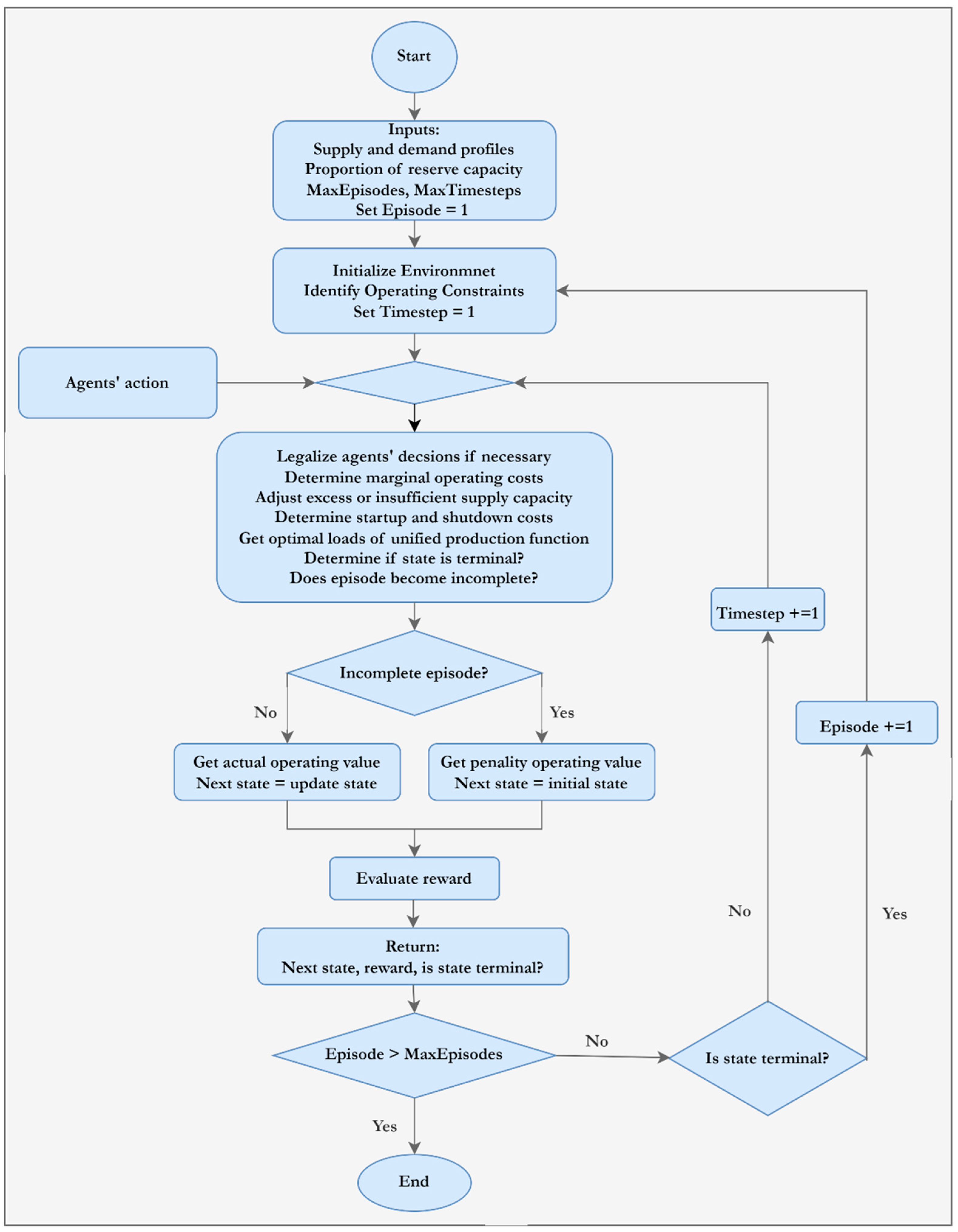
3.1. Multi-Agent Simulation Environment

The key elements of MARL satisfy the properties of an MDP [55]. Consequently, the MOPS dynamics can also be formulated as a 4-tuple $\left(\mathcal{S},\mathcal{A},\mathcal{P},\mathcal{R}\right)$ MDP that will be simulated within the multi-agent simulation environment, as described below.

[Step 0] Inputs: The environment should be provided with parameters of power-generating units, demand profile, weight hyperparameters, and other specifications (such as the type of optimization: single, bi-objective, or tri-objective).

[Step 1] Initialization: The environment is initialized with state as ${\mathit{s}}_0=\left(0,{\mathit{p}}_0^{min},{\mathit{p}}_0^{max},{\mathcal{t}}_0,d_1\right)$.

[Step 2] Constraints: Units failing to meet their minimum down time (${\mathcal{t}}_i^{down}$) are kept OFF ($u_{ti}^0=$1). Similarly, units not fulfilling their minimum up time (${\mathcal{t}}_i^{up}$) are constrained to be ON ($u_{ti}^1=$1). These constraints can be defined as follows:

$$u_{ti}^0=1 \mathrm{if}-{\mathcal{t}}_i^{down}<{\mathcal{t}}_{t-1,i}<0; u_{ti}^1=1 \mathrm{if} 0<{\mathcal{t}}_{t-1,i}<{\mathcal{t}}_i^{up}; \forall i.$$

(19)

[Step 3] Startup and shutdown values: Startup cost is determined based on the duration during which a unit has been continuously offline (OFF) until a certain timestep $t$. This cost is commonly approximated using a staircase function given as follows:

$${\mathcal{C}}_{ti}^{su}=\left\{\begin{array}{l}{\mathcal{C}}_i^{hot}, if-\left({\mathcal{t}}_i^{down}+{\mathcal{t}}_i^{cold}\right)\le {\mathcal{t}}_{t-1,i}\le -{\mathcal{t}}_i^{down}\\ {\mathcal{C}}_i^{cold}, if {\mathcal{t}}_{t-1,i}<-\left({\mathcal{t}}_i^{down}+{\mathcal{t}}_i^{cold}\right) \end{array};\forall i\right..$$

(20)

On the other hand, startup emissions $\left({\mathcal{E}}_{ti}^{su}\right)$, shutdown costs $\left({\mathcal{C}}_{ti}^{su}\right)$, and shutdown emissions $\left({\mathcal{E}}_{ti}^{sd}\right)$ are all assumed to be zero as usual in the existing literature.

[Step 4] Transition {$\mathcal{P}\left({\mathit{s}}_t|{\mathit{s}}_{t-1},{\mathcal{a}}_{t-1}\right)\}$: At each state ${\mathit{s}}_{t-1}$, the transition function will receive the decision ${\mathcal{a}}_{t-1}$ of all $n$ agents as an input. The transition function plays a critical role in ensuring that the MARL framework aligns with the constraints of the MOPS problem. Accordingly, the legality of each agent’s decision is verified first based on the constraints determined in Equation (19). The collective decisions are subsequently assessed to confirm if the total supply capacity can meet the demand required, including reserve, for that timestep. Details of these adjustments are explained below.

[Step 4.1] Legalize agents’ decisions: Upon receiving the action ${\mathcal{a}}_{t-1}$ of agents, the transition function will scrutinize the legality of each agent’s decision ${\mathcal{a}}_{t-1,i}\in {\mathcal{a}}_{t-1}$. Any agent’s decision conflicting with Equation (19) is corrected as follows:

$${\mathcal{a}}_{t-1,i}=1 \mathrm{if} {\mathcal{a}}_{t-1,i}=0 | u_{ti}^1=1; {\mathcal{a}}_{t-1,i}=0 \mathrm{if} {\mathcal{a}}_{t-1,i}=1 | u_{ti}^0=0; \forall i.$$

(21)

Equation (21) represents the appropriate adjustments to be made if there are ON units that should have been OFF, or vice versa.

[Step 4.2] Priority list: To facilitate capacity adjustments, priority list approaches [38,39,40] are usually adopted. Existing priority list methods are limited to increasing cost and emission functions. These methods additionally disregard startup and shutdown impacts. To address these limitations, this study has made some adjustments. First, the minimum marginal production values per MW of the individual objectives are modified as follows:

$${\lambda }_{ik}^{min}=\frac{1}{p_i^{max}}{\mathcal{O}}_k^{on}\left(p_i\right);\forall i,k \mathrm{where} p_i=\left\{\begin{array}{c}{p}_i^{max}, if {\mathcal{O}}_k^{on}\left(p_i^{max}\right)\ge {\mathcal{O}}_k^{on}\left(p_i^{min}\right)\\ p_i^{min}, if {\mathcal{O}}_k^{on}\left(p_i^{max}\right)<{\mathcal{O}}_k^{on}\left(p_i^{min}\right)\end{array}\right.;\forall i,k.$$

(22)

Equation (22) accounts for the trends of cost and emissions functions, but it does not incorporate units’ startup and shutdown impacts. By incorporating startup and shutdown impacts together with the minimum up- and down-time durations, Equation (23) determines the minimum marginal operating values for each objective.

$${\mathsf{\Lambda }}_{ik}^{min}={\lambda }_{ik}^{min}+\frac{1}{p_i^{max}}\left[{\mathcal{a}}_{t-1,i}⟦{\mathcal{t}}_{t-1,i}<0⟧\frac{{\mathcal{O}}_{tik}^{su}}{{\mathcal{t}}_i^{up}}+\left(1-{\mathcal{a}}_{t-1,i}\right)⟦{\mathcal{t}}_{t-1,i}>0⟧\frac{{\mathcal{O}}_{tik}^{sd}}{{\mathcal{t}}_i^{down}}\right];\forall i,k.$$

(23)

The priority list corresponding to the MOPS objective function can be obtained by averaging the priority values of the individual objectives, defined as follows:

$${\mathsf{\Lambda }}_i^{min}=\frac{1}{m+1}\sum _{k=0}^m{\mathsf{\Lambda }}_{ik}^{min};\forall i.$$

(24)

[Step 4.3] Capacity adjustments: Based on the order of values in Equation (24), the simulation environment orchestrates capacity adjustments to ensure a reliable power supply that satisfies current and future demands. First, there may be cases where future demands $d_{t^{\mathrm{*}}};\left(t<t^{\mathrm{*}}<24\right)$ cannot be met during the downtime of some units. Those units must remain online, even if they have fulfilled their minimum uptime durations. Second, the simulation environment will be able to manage both excess and shortage of power supply capacities as follows:

• If there is a shortage of capacity (i.e., $\sum _{i=1}^n{\mathcal{a}}_{t-1,i}{p}_{t-1,i}^{max}<\left[1+\mathcal{r}\right]d_t$), unconstrained OFF units are turned ON (${\mathcal{a}}_{t-1,i}=1|u_{ti}^1=0$) in the increasing order of ${\mathsf{\Lambda }}_i^{min}$ until the demand, including reserve, is met (i.e., $\sum _{i=1}^n{\mathcal{a}}_{t-1,i}{p}_{t-1,i}^{max}\ge \left[1+\mathcal{r}\right]d_t$) or no unconstrained OFF unit remains.
• If there is excess capacity (i.e., $\sum _{i=1}^n{\mathcal{a}}_{t-1,i}{p}_{t-1,i}^{min}>\left[1+\mathcal{r}\right]d_t$), unconstrained ON units are turned OFF (${\mathcal{a}}_{t-1,i}=0|u_{t-1,i}^0=1$) in the decreasing order of ${\mathsf{\Lambda }}_i^{min}$ until supply matches demand, including reserve (i.e., $\sum _{i=1}^n{\mathcal{a}}_{t-1,i}{p}_{t-1,i}^{min}\le \left[1+\mathcal{r}\right]d_t$) or no unconstrained ON units are left.

[Step 4.4] Optimal loads of MOPS production function: The optimal loads in the unified production function ${\Phi }^{on}\left(p_{ti}\right)$ defined in Equation (7) can be determined using sequential least squares programming (SLSP) [56]. These loads $p_{ti},\forall i$ can be determined as follows:

$${\mathit{p}}_t=\underset{p_{t1},p_{t2},\dots ,p_{tn}}{\mathrm{a}\mathrm{r}\mathrm{g}\mathrm{m}\mathrm{i}\mathrm{n}}{\Phi }^{on}\left(p_{t1},p_{t2}\dots ,p_{tn}\right).$$

(25)

[Step 4.5] Incomplete episode and terminal state: Complete episodes share the same terminal state $\left({\mathit{s}}_{23}^{+}\right)$, possibly with different state values. However, determining unit commitments and load dispatches for all timesteps is not always feasible. Despite the contextual correction capabilities of the simulation environment, certain scenarios may pose challenges. There might not be enough unconstrained ON units to switch OFF to adjust excess capacity. Conversely, there might not be enough unconstrained OFF units to switch ON during a supply shortage. In such situations, transitioning from the current state ${\mathit{s}}_{t-1}$ to the next succeeding state ${\mathit{s}}_t$ is not possible, and this state ${\mathit{s}}_{t-1}$ is also designated as a terminal state (i.e., ${\mathit{s}}_{t-1}^{+}$). This renders the corresponding episode incomplete. In other words, an episode is incomplete if $⟦{\mathit{s}}_{t-1}^{+}⟧=1$ whenever $t<24$. It should be noted that the terminal state varies from episode to episode, resulting in the number of timesteps across episodes being a random variable [55].

[Step 4.6] Total operating values of individual objective functions: The total operating value ${\mathcal{O}}_{tk}$ of objective $k$ is calculated by summing its startup, shutdown, and production values, which can be written as follows:

$${\mathcal{O}}_{tk}=\sum _{i=1}^n\left[{\mathcal{a}}_{t-1,i} {\mathcal{O}}_k^{on}\left(p_{ti}\right)+{\mathcal{a}}_{t-1,i}⟦{\mathcal{t}}_{t-1,i}<0⟧{\mathcal{O}}_{tik}^{su}+{\mathcal{a}}_{t-1,i}⟦{\mathcal{t}}_{ti}>0⟧{\mathcal{O}}_{tik}^{sd}\right],\forall k$$

(26)

where the production value ${\mathcal{O}}_k^{on}\left(p_{ti}\right)$ is evaluated at the optimal loads determined in Equation (25). In episodic decision-making scenarios, it is usually needed to prevent incomplete episodes. To ensure this, large penalties are often recommended [5]. In this study, the penalty imposed ensures that episodes with fewer timesteps incur higher operating values, underscoring the significance of complete episodes for effective learning and decision-making. This penalty can be defined as follows:

$${\mathcal{O}}_{tk}=\sum _{i=1}^n{\mathcal{O}}_k^{on}\left(p_i^{max}\right)+\frac{t-1}{23}\left[{\mathcal{O}}_k^{on,max}-\sum _{i=1}^n{\mathcal{O}}_k^{on}\left(p_i^{max}\right)\right];\forall k$$

(27)

where ${\mathcal{O}}_k^{on}\left(p_i^{max}\right)$ represents the maximum capacity production value and ${\mathcal{O}}_k^{on,max}$ denotes the maximum possible production value, which is computed as ${\mathcal{O}}_k^{on,max}=\sum _{i=1}^n{\lambda }_{ik}^{max}{p}_i^{max}$. Here, ${\lambda }_{ik}^{max}$ is given as follows:

$${\lambda }_{ik}^{max}=\frac{1}{p_i^{min}}{\mathcal{O}}_k^{on}\left(p_i\right) \mathrm{where} p_i=\left\{\begin{array}{c}{p}_i^{min}, if p_i^{min}\ge -\frac{\beta }{2\alpha }\\ -\frac{\beta }{2\alpha }, if p_i^{min}<-\frac{\beta }{2\alpha }\end{array}\right.;\forall i.$$

(28)

Equation (28) is like Equation (22), but represents the maximum marginal production value per MW, considering the trends of the cost and emission functions. It is crucial to note that the actual operating cost in Equation (26) is utilized whenever $⟦{\mathit{s}}_{t-1}^{+}⟧=0$, while the penalty in Equation (27) is applied when the episode becomes incomplete (i.e., when $⟦{\mathcal{s}}_{t-1}^{+}⟧=1$ for $t<24$).

[Step 4.7] Determine the next state: Depending on the contextually corrected action ${\mathcal{a}}_{t-1}$ in state ${\mathit{s}}_{t-1}$, the simulation environment is initialized, or the subsequent state ${\mathit{s}}_t$ is obtained through updating ${\mathit{s}}_{t-1}$. Details of these scenarios are described in [42].

[Step 4.8] Reward function: The reward function $r_t=\mathcal{R}\left({\mathit{s}}_{t-1},{\mathcal{a}}_{t-1},{\mathit{s}}_t\right)$ is defined as the inversed average of the normalized values of all individual objectives. It can be represented as follows:

$$r_t={\left[\frac{1}{m+1}\sum _{k=0}^m\left(\frac{{\mathcal{O}}_{tk}-{\mathcal{O}}_k^{min}}{{\mathcal{O}}_k^{max}-{\mathcal{O}}_k^{min}}\right)\right]}^{-1}$$

(29)

where ${\mathcal{O}}_k^{min}$ represents the minimum possible production value, which is defined as ${\mathcal{O}}_k^{min}=\mathit{min}\left({\lambda }_{ik}^{min}{p}_i^{min};\forall i\in \mathfrak{T}\right)$.

[Step 5] Return: Executing action ${\mathcal{a}}_{t-1}$ in state ${\mathit{s}}_{t-1}$ in the transition function will mainly return a three-tuple (${\mathit{s}}_t$,$r_t,⟦{\mathit{s}}_{t-1}^{+}⟧$), where ${\mathit{s}}_t$ represents the next state, $r_t$ represents the reward defined in Equation (29), and $⟦{\mathit{s}}_{t-1}^{+}⟧$ is an indicator whether the current state is terminal. Additionally, the output includes unit commitments, optimal loads, and other related information.

[Step 6] Proceed to the next timestep or reset the environment: If $⟦{\mathit{s}}_{t-1}^{+}⟧$ = 0, the simulation continues to the next timestep of the episode, executing another action of agents in Step 4. However, if $⟦{\mathit{s}}_{t-1}^{+}⟧$ = 1, the simulation environment will be reset to its initial status (proceeding to Step 1) to start the next new episode. This ensures a clear distinction in the simulation process based on the completeness of the episodes.

Figure 1 summarizes the process of simulating the power scheduling dynamics in the form of MDPs, and the pseudocode is presented in Algorithm 1.

Algorithm 1. Pseudocode for simulating power scheduling as MDPs

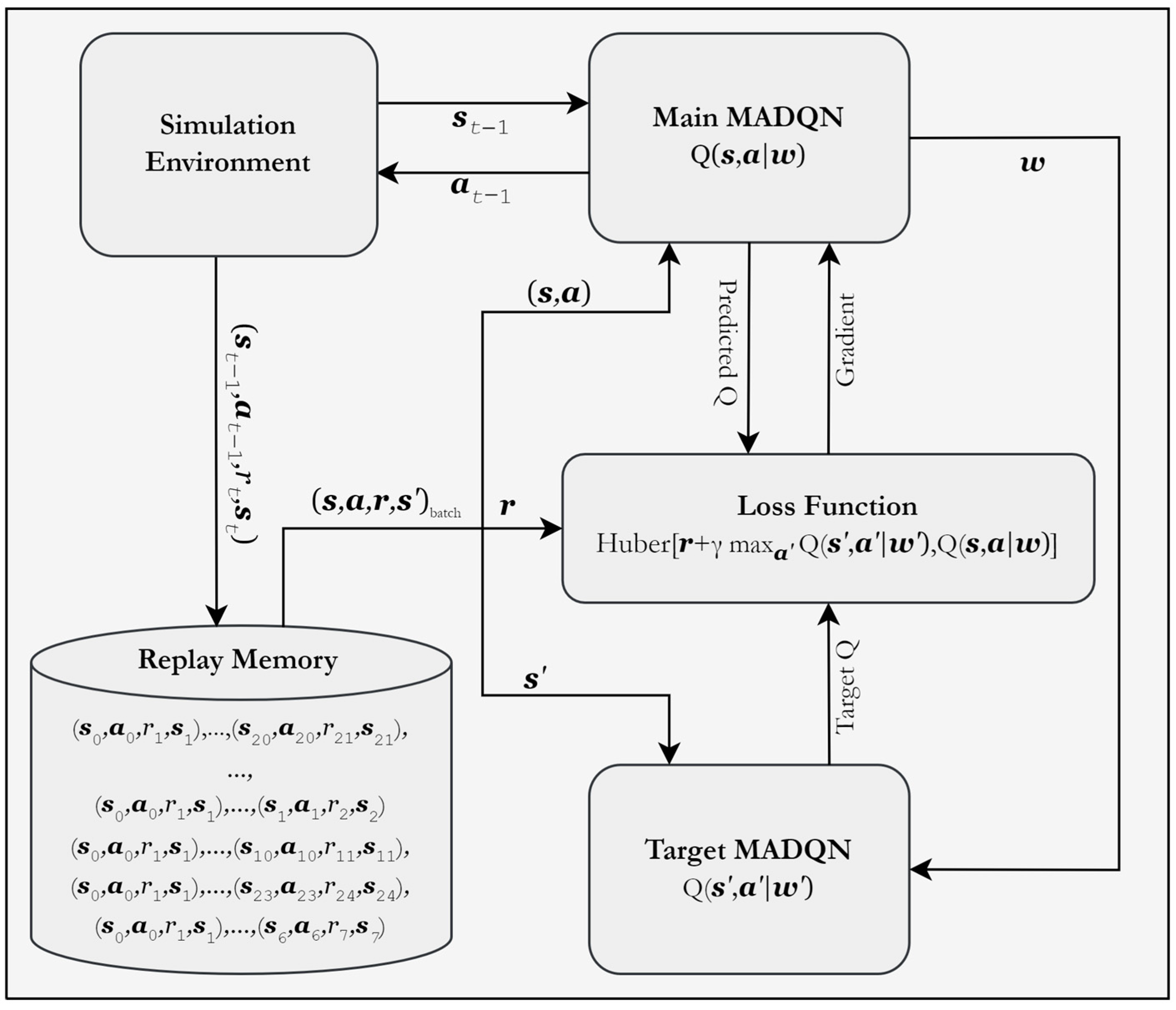
3.2. Multi-Agent Deep Q-Network (MADQN)

In the framework of RL, the transition function $\mathcal{P}\left({\mathit{s}}_t,r_t|{\mathit{s}}_{t-1},{\mathcal{a}}_{t-1}\right)$ defines the probability distribution of the next state ${\mathit{s}}_t$ with reward $r_t$ for taking an action ${\mathcal{a}}_{t-1}\in \mathcal{A}\left({\mathit{s}}_{t-1}\right)$ in state ${\mathit{s}}_{t-1}\in \mathcal{S}$. This mapping is called a policy $\pi \left({\mathcal{a}}_{t-1}|{\mathit{s}}_{t-1}\right)$ [55], which is a guide that helps the agents choose action ${\mathcal{a}}_{t-1}$ given the state ${\mathit{s}}_{t-1}$ at each timestep $t$ of an episode. The goal of the different cooperative agents is to learn a policy $\pi \left({\mathcal{a}}_{t-1}|{\mathit{s}}_{t-1}\right)$ that maximizes their long-run cumulative return (sum of rewards), determined as $G_t=\sum _{t=1}^T{\gamma }^{t-1}{r}_t$, where $\gamma$ is a discount rate $\left(0\le \gamma \le 1\right)$. The expected return of the state $V_{\pi }\left(\mathit{s}\right)$ following a policy $\pi$ is defined as $V_{\pi }\left(\mathit{s}\right)={\mathbb{E}}_{\pi }\left(G_t|{\mathit{s}}_{t-1}=\mathit{s}\right)$. Similarly, the action-value function $Q_{\pi }\left(\mathit{s},\mathcal{a}\right)$, representing the expected return of taking an action ${\mathcal{a}}_{t-1}$ in state ${\mathit{s}}_{t-1}$, is given by:

$$Q_{\pi }\left(\mathit{s},\mathcal{a}\right)={\mathbb{E}}_{\pi }\left(G_t|{\mathit{s}}_{t-1}=\mathit{s},{\mathcal{a}}_{t-1}=\mathcal{a}\right).$$

(30)

The optimal policy is now denoted as $\pi \left(\mathit{s}|\mathcal{a}\right)$ and is defined as $\pi \left(\mathit{s}|\mathcal{a}\right)=argma{x}_{\pi }{V}_{\pi }\left(\mathit{s}\right)$ for all $\mathit{s}\in \mathcal{S}$ or $\pi \left(\mathit{s}|\mathcal{a}\right)=argma{x}_{\pi }{Q}_{\pi }\left(\mathit{s},\mathcal{a}\right)$ for all $\mathcal{a}\in \mathcal{A}\left(\mathit{s}\right)$. As a result, the action value corresponding to the optimal policy is as follows:

$$Q_{\pi }^{*}\left(\mathit{s},\mathcal{a}\right)=\mathit{ma}{x}_{\pi }{Q}_{\pi }\left(\mathit{s},\mathcal{a}\right);\forall \left(\mathit{s},\mathcal{a}\right)\in \mathcal{S}\times \mathcal{A}$$

(31)

where $Q_{\pi }\left(\mathit{s},\mathcal{a}\right)$ represents the action value defined in Equation (30). However, calculating exact values as defined in Equation (31) for all state-action pairs $\left(\mathit{s},\mathcal{a}\right)$ is infeasible due to the exponential growth of the state-action pairs. Instead, these values can be estimated through function approximation methods [29]. This study employs a deep Q-network (DQN) to approximate the action value function. DQN is a robust technique as it does not require a precise mathematical definition of a loss function and can identify optimal solutions, even for nonconvex loss functions [29]. The specifics of the DQN model, including its network architecture, exploration strategy, loss function, and unique features, are detailed in [48].

3.2.1. Model Architecture

The DQN model employed in this study utilizes a single-hidden-layer feedforward neural network model with ReLU activation functions in both the hidden and output layers. The input of the network comprises the MDP dynamics represented by ${\mathit{s}}_{t-1}=\left(t,{\mathit{p}}_{t-1}^{min},{\mathit{p}}_{t-1}^{max},{\mathcal{t}}_{t-1},d_t\right)$, which are simulated within the multi-agent simulation environment. The network output represents the action value function $Q_{\pi }\left(\mathit{s},\mathcal{a}|\mathit{w}\right)$, where $\mathit{w}$ consists of the model’s weights. The model is designed to predict two values for each agent. In this setup, each pair of nodes corresponds to the two possible decisions (i.e., ON and OFF) for each of the $n$ agents. This approach is necessitated by the complexity of the action space $\mathcal{A}$, which inherently poses a formidable challenge due to its exponential growth concerning the number of agents involved (resulting in $2^n$ possible unit commitments). To mitigate this complexity, the network is designed with $2n$ output nodes, instead of parameterizing it into $2^n$ output nodes. This streamlined network parametrization is a strategic solution to handle the computational constraints posed by the exponential growth in the action space. This simplified network setup is strategic for managing computational complexity while ensuring an efficient modeling process. Importantly, the network design is decentralized, where each agent has a dedicated pair of output nodes. As a result, the DQN is referred to as the MADQN. This approach results in the network output becoming a linear function of the number of agents, enabling a more manageable and practical implementation within the multi-agent system.

In this framework, an $ϵ$-greedy exploration approach is used. Accordingly, agents autonomously make their optimal decision ${\mathcal{a}}_{t-1,i};\forall t$ within state ${\mathit{s}}_{t-1}$ with probability $1-ϵ$. Conversely, with probability $ϵ$, each agent explores the environment by deciding randomly. In both conditions, once the action ${\mathcal{a}}_{t-1}$ of all agents is formed, it serves as an input to the transition function in the simulation environment, initiating the next state ${\mathit{s}}_t$, which will be the input for the MADQN model.

It is noteworthy that while MADQN is used in this study, the multi-agent simulation environment is not specifically designed for a particular RL model. It remains adaptable, allowing for the training of various RL models based on user preferences.

3.2.2. Experience Relay

In the context of power scheduling problems, an action taken in a particular state affects the immediate reward and has repercussions on a sequence of future states. Such interdependence among the successive MDPs poses a challenge when applying the standard MADQN [5]. The MADQN can be enhanced by incorporating an experience replay to address this issue. Experience replay involves storing the transition tuples in a replay buffer, denoted as $\mathbb{B}=\left\{\left({\mathit{s}}_{t-1},{\mathcal{a}}_{t-1},r_t,{\mathit{s}}_t\right)\right\}$, and then using a random batch of experiences $\left(\mathit{s},\mathcal{a},\mathit{r},{\mathit{s}}^{\prime }\right)$ to estimate the action values. This approach helps break the temporal correlations among the MDPs [57]. By learning from random past experiences, the agents can more effectively explore the state-action space in diverse situations. This approach enhances the learning process by mitigating the challenges of autocorrelated sequential MDPs.

3.2.3. Loss Function and Parameter Updates

The choice of an appropriate loss function is crucial in RL to ensure stable and effective training of the model. To calculate the loss, MADQN incorporates target and main networks [45]. The target network generates target action values and is updated periodically from the primary network $Q\left(\mathit{s},\mathcal{a}|\mathit{w}\right)$. Its values are computed as $\mathit{r}+\gamma {\mathit{max}}_{{\mathcal{a}}^{\prime }}{Q}_{\pi }\left({\mathit{s}}^{\prime },{\mathcal{a}}^{\prime }|{\mathit{w}}^{\prime }\right)$, where ${\mathit{w}}^{\prime }$ is the weight of the target network. Due to the diverse variables present in the state input for the MADQN model, large errors in action-value estimates can occur, which may potentially lead to unstable training. In such situations, the Huber loss function proves to be more appropriate [55], which is expressed as:

$$J\left(\mathit{w}\right)=\mathbb{E}\left[\left\{\begin{array}{c}0.5{\left[\mathit{r}+\gamma \underset{{\mathit{a}}^{\prime }}{\mathit{max}}Q\left({\mathit{s}}^{\prime },{\mathcal{a}}^{\prime }|{\mathit{w}}^{\prime }\right)-Q\left(\mathit{s},\mathcal{a}|\mathit{w}\right)\right]}^2, if \left|\mathit{r}+\gamma \underset{{\mathit{a}}^{\prime }}{\mathit{max}}Q\left({\mathit{s}}^{\prime },{\mathcal{a}}^{\prime }|{\mathit{w}}^{\prime }\right)-Q\left(\mathit{s},\mathcal{a}|\mathit{w}\right)\right|<1\\ \left|\mathit{r}+\gamma \underset{{\mathit{a}}^{\prime }}{\mathit{max}}Q\left({\mathit{s}}^{\prime },{\mathcal{a}}^{\prime }|{\mathit{w}}^{\prime }\right)-Q\left(\mathit{s},\mathcal{a}|\mathit{w}\right)\right|-0.5, if \left|\mathit{r}+\gamma \underset{{\mathit{a}}^{\prime }}{\mathit{max}}Q\left({\mathit{s}}^{\prime },{\mathcal{a}}^{\prime }|{\mathit{w}}^{\prime }\right)-Q\left(\mathit{s},\mathcal{a}|\mathit{w}\right)\right|\ge 1\end{array}\right.\right]$$

(32)

where $\left(\mathit{s},\mathcal{a},\mathit{r},{\mathit{s}}^{\prime }\right)$ represent a batch of experiences sampled from the replay memory $\mathbb{B}$. The update rule for the network parameters is also expressed as:

$$\mathit{w}\leftarrow \mathit{w}+\xi \left(\mathit{r}+\gamma \underset{{\mathit{a}}^{\prime }}{\mathit{max}}Q\left({\mathit{s}}^{\prime },{\mathcal{a}}^{\prime }|{\mathit{w}}^{\prime }\right)-Q\left(\mathit{s},\mathcal{a}|\mathit{w}\right)\right)\nabla Q\left(\mathit{s},\mathcal{a}|\mathit{w}\right)$$

(33)

where $\xi$ is a learning rate. Huber loss can effectively handle different error values, ensuring stable learning [55]. It becomes an absolute error (i.e., L1 loss) for larger errors and resembles a mean-squared error (i.e., L2 loss) for small errors. This property of Huber loss enhances the model’s resilience to noisy data and outliers, leading to more reliable and stable training outcomes in the MADQN framework.

Figure 2 demonstrates how the multi-agent simulation environment and MADQN interact, combining the replay memory and loss function.

4. Practical Applications

The proposed MARL optimization algorithm addresses the MOPS problem with varying units and constraints. The implementation leverages the PyTorch deep learning framework, utilizing Python 3.10. It was executed on a desktop computer with an 11th Gen Intel (R) Core (TM) i7-11700 processor operating at 2.50 GHz, 16 GB of RAM, and eight parallel workers. In the write-up of the manuscript, while QuillBot has been used for language-related aspects, the substantive content and findings resulted from human intellectual effort.

4.1. Experimental Settings

4.1.1. Specifications of Generating Units

Profiles of the generating units, including the cost, emission, and ramp rate parameters, are taken from [54]. The VPE parameters of the cost functions are obtained from [58], and those of the emission functions are accessed from [21]. Moreover, the parameters specific to CO₂ and SO₂ for the tri-objective problems are drawn from [36]. Operational constraints, including generation capacity, minimum operating time durations, and a 10% reserve, remain the same across all test systems. Notably, shutdown costs and startup emissions are typically assumed to be negligible compared with other expenses [59], and their specific values are absent in the existing literature. Consequently, these parameters are uniformly set to zero in all the experimental analyses, although their integration into the algorithm’s framework has been duly considered. The proposed algorithm is not necessarily confined to a fixed timeframe. Despite this, all the experimental analyses are conducted over a 24 h planning horizon, with demand data from [54].

4.1.2. Parameters and Hyperparameters

The cost-to-emission conversion parameters significantly impact the optimization trade-offs between cost and emission objectives. Estimates of these parameters are presented in

Table 2. Estimates of cost-to-emission conversion parameters of generating units.

	$\mathit{\eta }$	U1	U2	U3	U4	U5	U6	U7	U8	U9	U10
Without VPEs	$\mathcal{C}$$-\mathrm{to}-\mathcal{E}$	1.12	1.12	1.18	1.72	1.32	1.60	1.42	0.63	0.64	0.63
	$\mathcal{C}$$-\mathrm{to}-{\mathcal{E}}^{C{O}_2}$	1.26	1.31	1.97	1.47	1.36	1.80	2.00	2.58	2.35	3.42
	$\mathcal{C}$$-\mathrm{to}-{\mathcal{E}}^{S{O}_2}$	4.64	4.98	4.00	3.74	5.23	3.51	7.16	2.64	2.63	2.67
With VPEs	$\mathcal{C}$$-\mathrm{to}-\mathcal{E}$	1.09	1.11	1.15	1.64	1.29	1.53	1.42	0.63	0.62	0.60

, which are calculated using Equation (16). The other crucial factors affecting MOPS optimization are the weight hyperparameters assigned to the different objectives. These weights are determined before fine-tuning the hyperparameters of the neural network model. As previously noted, the MADQN model utilized a single-hidden-layer neural network incorporating ReLU activation functions in both the hidden and output layers. With a preliminary configuration of the model, a thorough sensitivity analysis is conducted using fuzzy set theory. First, each objective function is individually optimized. Next, a set of 100 evenly distributed weights, ranging from 0 to 1, is considered for the bi-objective problems. Then, a membership function is created for each objective function using Equation (17), and the cardinality values are determined using Equation (18). The results of the top 10 weights with the largest cardinality values for the first 4 test systems are presented in

Table 3. Top ten weights with the largest cardinality values for the bi-objective problems.

Test System		1	2	3	4	5	6	7	8	9	10
I	$\omega$	0.35	0.36	0.37	0.38	0.39	0.40	0.41	0.42	0.43	0.44
	$\mu \left(\mathcal{C}\right)$	0.878007	0.890443	0.901638	0.912586	0.921031	0.928662	0.935648	0.942570	0.949212	0.955643
	$\mu \left(\mathcal{E}\right)$	0.207331	0.273058	0.252767	0.232082	0.215422	0.199729	0.184779	0.169305	0.153849	0.138279
	$\mu \left(\mathcal{C},\mathcal{E}\right)$	0.009882	0.010593	0.010510	0.010422	0.010347	0.010274	0.010201	0.010123	0.010043	0.009960
II	$\omega$	0.37	0.38	0.39	0.40	0.41	0.42	0.43	0.44	0.45	0.46
	$\mu \left(\mathcal{C}\right)$	0.898268	0.909701	0.917872	0.925332	0.932428	0.939034	0.945612	0.951902	0.957516	0.953013
	$\mu \left(\mathcal{E}\right)$	0.161389	0.236437	0.220693	0.205621	0.190679	0.176148	0.161154	0.146186	0.132335	0.135774
	$\mu \left(\mathcal{C},\mathcal{E}\right)$	0.009876	0.010682	0.010611	0.01054	0.010467	0.010393	0.010315	0.010234	0.010157	0.010147
III	$\omega$	0.30	0.36	0.37	0.40	0.45	0.48	0.62	0.91	0.92	0.95
	$\mu \left(\mathcal{C}\right)$	0.000001	0.000001	0.040960	0.075624	0.083236	0.098914	0.252296	0.207296	0.306373	0.260789
	$\mu \left(\mathcal{E}\right)$	0.311485	0.301039	0.273215	0.237354	0.220239	0.218529	0.058457	0.109696	0.011730	0.043777
	$\mu \left(\mathcal{C},\mathcal{E}\right)$	0.009821	0.009492	0.009906	0.009868	0.009569	0.010009	0.009798	0.009995	0.010030	0.009603
IV	$\omega$	0.42	0.54	0.68	0.69	0.70	0.73	0.87	0.96	0.97	0.98
	$\mu \left(\mathcal{C}\right)$	0.144462	0.110142	0.213309	0.216820	0.186339	0.208077	0.196714	0.222655	0.225096	0.164261
	$\mu \left(\mathcal{E}\right)$	0.087651	0.115980	0.013510	0.015474	0.000001	0.000001	0.000001	0.006746	0.000001	0.000001
	$\mu \left(\mathcal{C},\mathcal{E}\right)$	0.006831	0.006655	0.006676	0.006837	0.005484	0.006124	0.005790	0.006752	0.006625	0.004834

. In the context of tri-objective scheduling problems, a set of 200 random combinations of weights is sampled from the Dirichlet probability distribution.

Table 4. Top ten weights with the largest cardinality values for the tri-objective problems.

Test System		1	2	3	4	5	6	7	8	9	10
V	${\omega }^{cost}$	0.07	0.13	0.15	0.17	0.31	0.43	0.46	0.47	0.56	0.61
	${\omega }^{C{O}_2}$	0.67	0.60	0.57	0.52	0.38	0.21	0.22	0.17	0.06	0.06
	${\omega }^{S{O}_2}$	0.26	0.27	0.28	0.31	0.31	0.36	0.32	0.36	0.38	0.33
	$\mu \left(\mathcal{C}\right)$	0.877544	0.874737	0.876852	0.867023	0.876270	0.866799	0.882510	0.869905	0.863371	0.884918
	$\mu \left({\mathcal{E}}^{C{O}_2}\right)$	0.515861	0.518307	0.525821	0.513806	0.549959	0.560309	0.583100	0.572289	0.579697	0.612661
	$\mu \left({\mathcal{E}}^{S{O}_2}\right)$	0.617123	0.625220	0.620835	0.643178	0.624359	0.644600	0.610428	0.637967	0.650002	0.603679
	$\mu \left(\mathcal{C},\mathcal{E}\right)$	0.005176	0.005175	0.005211	0.005130	0.005298	0.005302	0.005445	0.005358	0.005361	0.005563
VI	${\omega }^{cost}$	0.03	0.21	0.24	0.41	0.43	0.44	0.45	0.49	0.52	0.52
	${\omega }^{C{O}_2}$	0.76	0.52	0.47	0.28	0.21	0.23	0.19	0.15	0.12	0.12
	${\omega }^{S{O}_2}$	0.21	0.26	0.29	0.31	0.36	0.33	0.35	0.36	0.36	0.36
	$\mu \left(\mathcal{C}\right)$	0.890529	0.885126	0.878897	0.882360	0.866862	0.878171	0.871210	0.870520	0.872000	0.871944
	$\mu \left({\mathcal{E}}^{C{O}_2}\right)$	0.530925	0.548683	0.542729	0.575160	0.561762	0.573672	0.569808	0.576117	0.582108	0.583029
	$\mu \left({\mathcal{E}}^{S{O}_2}\right)$	0.580650	0.601661	0.617481	0.610705	0.644421	0.620414	0.635385	0.636538	0.633200	0.633290
	$\mu \left(\mathcal{C},\mathcal{E}\right)$	0.005296	0.005342	0.005297	0.005431	0.005323	0.005410	0.005369	0.005390	0.005418	0.005421

provides the top 10 weight combinations, each possessing the highest cardinality values.

4.1.3. MADQN Model Configurations

Following the selection of promising weights for the different objectives, the hyperparameters of the MADQN are tuned. In the network configuration, generation capacities were initially assumed to be included as part of the model’s input when ramp rate constraints were considered. However, integrating these generation capacities into state input destabilizes training stability. Consequently, the input layer in all the test system models consists of $\left(n+2\right)$ nodes, encompassing three elements: the timestep of the planning horizon, the operating time durations, and the demand requirement to be satisfied. All the test systems employed a uniform learning rate of 0.01 and a consistent discount factor of 0.99. The optimization has been performed with the Adam optimizer and the Huber loss function. Furthermore, the exploration–exploitation strategy involves a maximum exploration rate set at 1 and a minimum rate of 0. An exponential decay rate associated with the number of training episodes determines the gradual reduction in exploration as the model’s training progresses. As the model employs experience replay, the batch size is consistently set to match the size of replay memory. The uniformity ensures a consistent approach to learning and updating the model parameters across different scenarios.

Table 5. Parameters and optimal hyperparameters of the MADQN models.

Test System	Objectives	Units	Nodes			$\in$-Decay Rate	Replay Memory	Training Episodes
			Input	Hidden	Output
I	Bi-objective	10	12	64	20	0.999	64	8000
II	Bi-objective	10	12	64	20	0.999	64	8000
III	Bi-objective	10	12	64	20	0.999	64	8000
IV	Bi-objective	10	12	64	20	0.999	64	8000
V	Tri-objective	10	12	64	20	0.9991	64	10,000
VI	Tri-objective	10	12	64	20	0.9991	64	10,000
VII–X	Bi-objective	20	22	64	40	0.999	64	8000
XI–XIV	Bi-objective	40	42	128	80	0.9993	128	12,000
XV–XVIII	Bi-objective	60	62	128	120	0.9993	128	12,000
XIX–XXII	Bi-objective	80	82	256	160	0.9994	256	15,000
XXIII–XXVI	Bi-objective	100	102	256	200	0.9994	256	15,000

shows the parameters and optimal hyperparameters of the MADQN models for the different test systems.

4.2. Comparative Results

4.2.1. Test System I: Bi-Objective Problem without Ramp Rate Constraints and No VPEs

Test system I comprises 10 generating units, each with smooth and convex cost and emission functions. The unit commitments, loads, and actual reserve percentages resulting from the proposed MADRL algorithm are presented in

Table 6. Optimal commitments, loads, and reserve percentages using MADRL for test system I.

$\mathit{t}$ (Hour)	Commitments	Optimal Loads (MW)										$\mathcal{r}\left(\mathit{\%}\right)$
		${\mathit{p}}_{\mathit{t}1}$	${\mathit{p}}_{\mathit{t}2}$	${\mathit{p}}_{\mathit{t}3}$	${\mathit{p}}_{\mathit{t}4}$	${\mathit{p}}_{\mathit{t}5}$	${\mathit{p}}_{\mathit{t}6}$	${\mathit{p}}_{\mathit{t}7}$	${\mathit{p}}_{\mathit{t}8}$	${\mathit{p}}_{\mathit{t}9}$	${\mathit{p}}_{\mathit{t},10}$
1	1100000000	375.8	324.2	0	0	0	0	0	0	0	0	30.0
2	1100000000	400.6	349.4	0	0	0	0	0	0	0	0	21.3
3	1100100000	405.5	354.3	0	0	90.2	0	0	0	0	0	26.1
4	1100100000	442.5	391.7	0	0	115.9	0	0	0	0	0	12.8
5	1101100000	412.9	361.8	0	130.0	95.4	0	0	0	0	0	20.2
6	1111100000	401.8	350.5	130.0	130.0	87.7	0	0	0	0	0	21.1
7	1111100000	420.3	369.2	130.0	130.0	100.5	0	0	0	0	0	15.8
8	1111100000	438.8	387.9	130.0	130.0	113.3	0	0	0	0	0	11.0
9	1111111000	455.0	409.4	130.0	130.0	128.0	21.7	25.9	0	0	0	15.2
10	1111111100	455.0	441.4	130.0	130.0	149.9	37.7	28.5	27.5	0	0	10.9
11	1111111110	455.0	454.1	130.0	130.0	158.7	44.1	29.5	29.6	18.9	0	10.8
12	1111111111	455.0	455.0	130.0	130.0	162.0	58.4	31.8	34.5	23.9	19.3	10.8
13	1111111100	455.0	441.4	130.0	130.0	149.9	37.7	28.5	27.5	0	0	10.9
14	1111111000	455.0	409.4	130.0	130.0	128.0	21.7	25.9	0	0	0	15.2
15	1111100000	438.8	387.9	130.0	130.0	113.3	0	0	0	0	0	11.0
16	1111100000	383.3	331.8	130.0	130.0	74.8	0	0	0	0	0	26.9
17	1111100000	364.8	313.1	130.0	130.0	62.0	0	0	0	0	0	33.2
18	1111100000	401.8	350.5	130.0	130.0	87.7	0	0	0	0	0	21.1
19	1111100000	438.8	387.9	130.0	130.0	113.3	0	0	0	0	0	11.0
20	1111111100	455.0	441.4	130.0	130.0	149.9	37.7	28.5	27.5	0	0	10.9
21	1111111000	455.0	409.3	130.0	130.0	128.0	21.7	25.9	0	0	0	15.2
22	1100111000	455.0	435.8	0	0	146.1	35.0	28.1	0	0	0	12.5
23	1100100000	424.0	373.0	0	0	103.1	0	0	0	0	0	19.1
24	1100000000	425.5	374.5	0	0	0	0	0	0	0	0	13.7

. The results of the proposed MADRL approach are compared with those of [23,34]. The former employed TLBO and achieved a daily operating cost of $578,445.5 with an emission of 37,302.9 lbs, while the proposed MADRL results in an operating cost of $563,990.6 and an emission level of 41,310.4 lbs. If economic considerations, which are critical in various industrial and business applications, are paramount, MADRL may be preferred. On the other hand, if environmental concerns take precedence, TLBO might be considered. As a multi-objective optimization problem, MADRL strikes a reasonable balance between operating costs and environmental emissions. Hence, the higher daily operating cost for a slightly lower emission introduced by TLBO makes its solutions less viable from an economic standpoint.

Conversely, RCGWO was adopted in [34], which reported a daily operating cost of $568,655.3 and an emission of 43,759.7 lbs.

Table 7. Comparison of costs and emissions between RCGWO and MADRL for test system I.

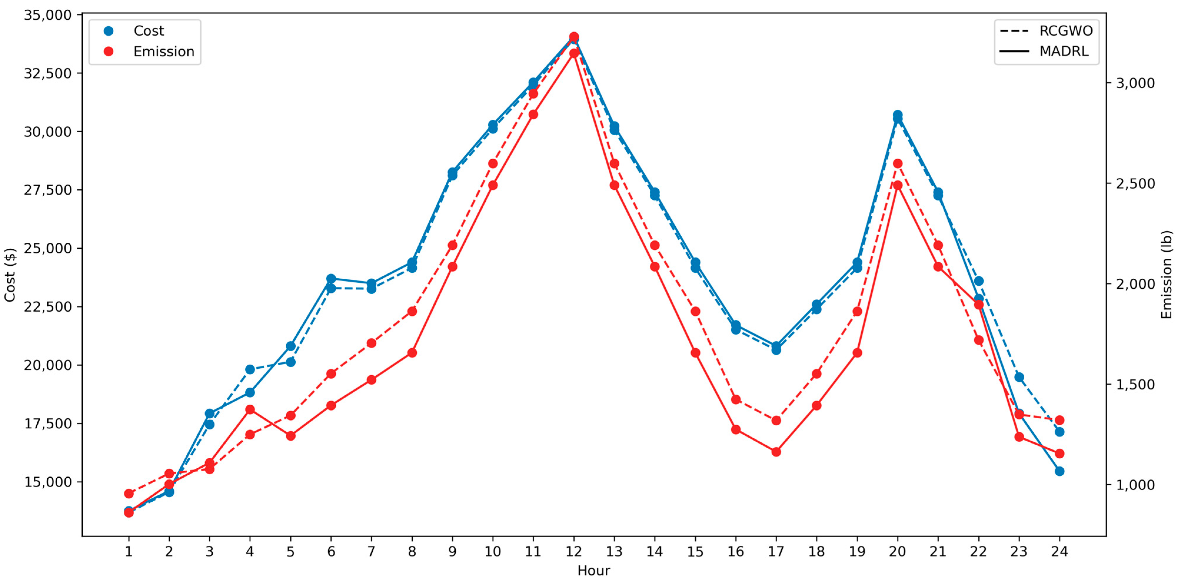
$\mathit{t}$ (Hour)	RCGWO [34]				MADRL
	${\mathcal{C}}_{\mathit{t}}^{\mathit{s}\mathit{u}}$ ($)	${\mathcal{C}}_{\mathit{t}}^{\mathit{o}\mathit{n}}$ ($)	${\mathcal{C}}_{\mathit{t}}$ ($)	${\mathcal{E}}_{\mathit{t}}$ (lbs)	${\mathcal{C}}_{\mathit{t}}^{\mathit{s}\mathit{u}}$ ($)	${\mathcal{C}}_{\mathit{t}}^{\mathit{o}\mathit{n}}$ ($)	${\mathcal{C}}_{\mathit{t}}$ ($)	${\mathcal{E}}_{\mathit{t}}$ (lbs)
1	0	13,683.1	13,683.1	956.4	0	13,750.3	13,750.3	861.1
2	0	14,554.5	14,554.5	1055.0	0	14,601.2	14,601.2	1002.2
3	560	16,892.1	17,452.1	1077.4	900	17,027.5	17,927.5	1108.7
4	550	19,261.5	19,811.5	1249.8	0	18,821.2	18,821.2	1373.8
5	0	20,132.5	20,132.5	1343.8	560	20,246.3	20,806.3	1243.5
6	900	22,387.1	23,287.1	15,52.7	1100	22,601.0	23,701.0	1394.3
7	0	23,262.0	23,262.0	1704.2	0	23,496.6	23,496.6	1521.4
8	0	24,150.3	24,150.3	1863.1	0	24,394.0	24,394.0	1656.3
9	860	27,251.1	28,111.1	2191.3	860	27,399.1	28,259.1	2085.1
10	60	30,057.6	30,117.6	2599.2	60	30,226.2	30,286.2	2490.5
11	60	31,916.1	31,976.1	2945.2	60	32,045.6	32,105.6	2843.0
12	60	33,890.2	33,950.2	3229.4	60	33,995.6	34,055.6	3146.4
13	0	30,057.6	30,057.6	2599.2	0	30,226.2	30,226.2	2490.5
14	0	27,251.1	27,251.1	2191.3	0	27,399.1	27,399.1	2085.1
15	0	24,150.3	24,150.3	1863.1	0	24,394.0	24,394.0	1656.3
16	0	21,513.7	21,513.7	1424.2	0	21,707.3	21,707.3	1274.9
17	0	20,641.8	20,641.8	1318.6	0	20,815.4	20,815.4	1163.3
18	0	22,387.1	22,387.1	1552.7	0	22,601.0	22,601.0	1394.3
19	0	24,150.3	24,150.3	1863.1	0	24,394.0	24,394.0	1656.3
20	490	30,057.6	30,547.6	2599.2	490	30,226.2	30,716.2	2490.5
21	0	27,251.1	27,251.1	2191.3	0	27,399.1	27,399.1	2085.1
22	0	23,593.0	23,593.0	1719.6	0	22,847.1	22,847.1	1895.6
23	0	19,480.8	19,480.8	1348.9	0	17,923.5	17,923.5	1237.4
24	0	17,142.8	17,142.8	1321.1	0	15,453.1	15,453.1	1154.8
Total	3540	565,115.3	568,655.3	43,759.7	4090.0	563,990.6	568,080.6	41,310.4

presents a detailed comparative analysis of outcomes obtained by the proposed MADRL methodology and the RCGWO [34] method. The hourly costs and emissions of both methods are also visualized in Figure 3. The slightly higher startup cost with the MADRL algorithm indicates an increase in the number of committed units. However, the efficiency of MADRL is demonstrated with a lower daily production cost of $563,990.6 compared with the cost of $565,115.3 using RCGWO. This economic efficiency positions MADRL as a promising solution. Furthermore, MADRL established a new environmental benchmark, emitting only 41,310.4 lbs of pollutants compared with RCGWO’s 43,759.7 lbs. Particularly noteworthy is the substantial reduction in hourly emissions, emphasizing the environmental conscientiousness of MADRL alongside its economic prowess. Excelling in both economic viability and environmental responsibility, the results underscore the holistic efficiency of MADRL.

4.2.2. Test System II: Ramp Rates Constrained Bi-Objective Problem without VPEs

Test system II is like test system I, except it is ramp rate constrained. No additional units are committed compared to the optimal schedule without ramp rate constraints. However, the dispatches of online generating units are strategically altered due to the inclusion of ramp rate constraints, which leads to changes in both operating costs and emissions. The results of the proposed MADRL and RCGWO [34] are shown in

Table 8. Comparison of costs and emissions between RCGWO and MADRL for test system II.

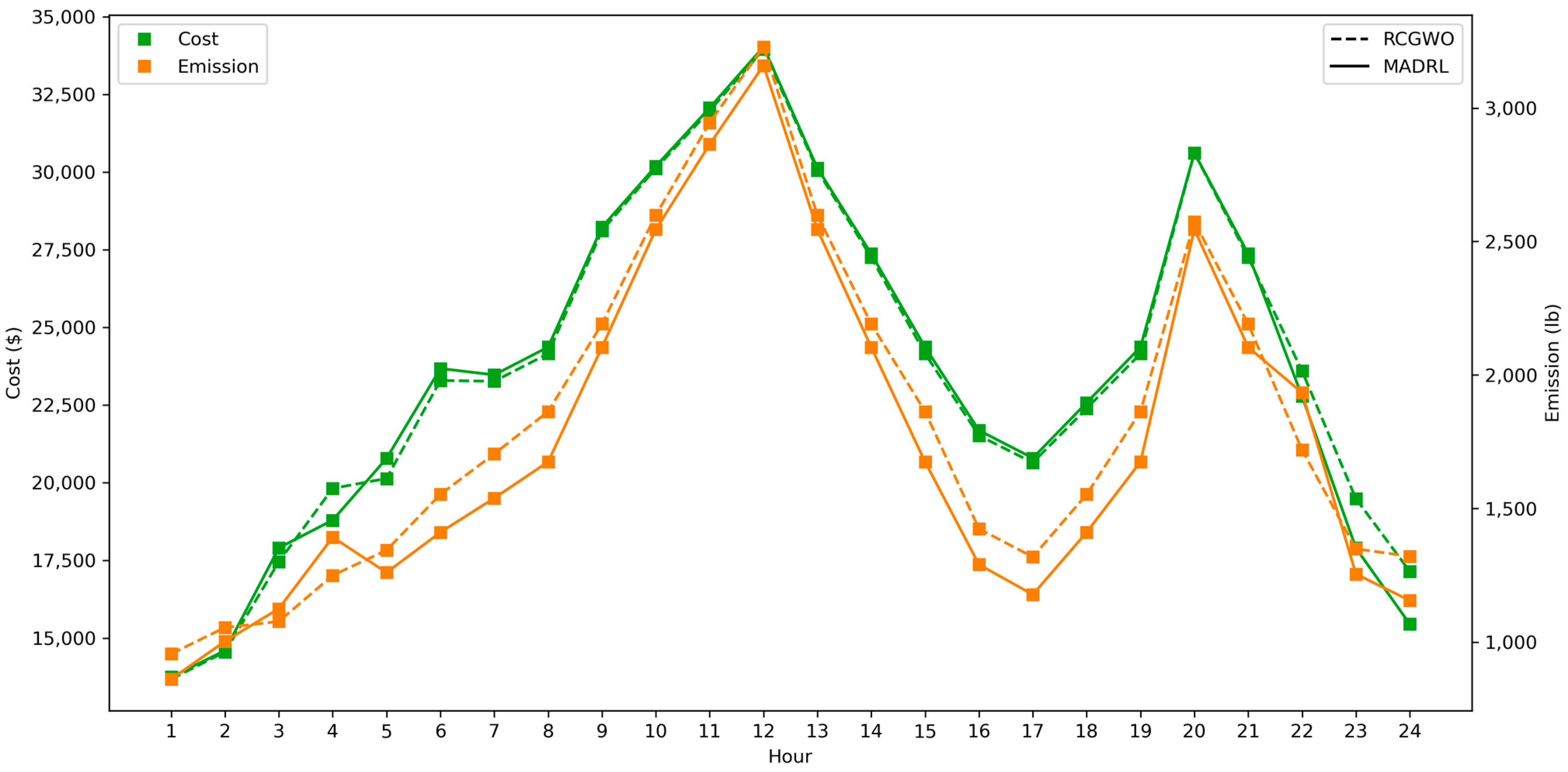
$\mathit{t}$ (Hour)	RCGWO [34]				MADRL
	${\mathcal{C}}_{\mathit{t}}^{\mathit{s}\mathit{u}}$ ($)	${\mathcal{C}}_{\mathit{t}}^{\mathit{o}\mathit{n}}$ ($)	${\mathcal{C}}_{\mathit{t}}$ ($)	${\mathcal{E}}_{\mathit{t}}$ (lbs)	${\mathcal{C}}_{\mathit{t}}^{\mathit{s}\mathit{u}}$ ($)	${\mathcal{C}}_{\mathit{t}}^{\mathit{o}\mathit{n}}$ ($)	${\mathcal{C}}_{\mathit{t}}$ ($)	${\mathcal{E}}_{\mathit{t}}$ (lbs)
1	0	13,683.0	13,683.0	956.4	0	13,748.3	13,748.3	862.1
2	0	14,554.4	14,554.4	1055.0	0	14,599.3	14,599.3	1003.2
3	560	16,892.0	17,452.0	1077.3	900	16,998.9	17,898.9	1125.3
4	550	19,261.4	19,811.4	1249.8	0	18,789.8	18,789.8	1392.3
5	0	20,132.4	20,132.4	1343.8	560	20,217.1	20,777.1	1260.5
6	900	22,387.2	23,287.2	1552.7	1100	22,572.7	23,672.7	1410.7
7	0	23,262.1	23,262.1	1704.3	0	23,466.8	23,466.8	1538.7
8	0	24,150.1	24,150.1	1863.1	0	24,362.9	24,362.9	1674.5
9	860	27,251.3	28,111.3	2191.3	860	27,365.0	28,225.0	2103.9
10	60	30,057.8	30,117.8	2599.2	60	30,128.4	30,188.4	2545.2
11	60	31,916.3	31,976.3	2945.2	60	32,008.3	32,068.3	2864.0
12	60	33,890.4	33,950.4	3229.4	60	33,972.9	34,032.9	3159.7
13	0	30,057.8	30,057.8	2599.2	0	30,128.5	30,128.5	2545.2
14	0	27,251.3	27,251.3	2191.3	0	27,365.0	27,365.0	2103.9
15	0	24,150.1	24,150.1	1863.1	0	24,362.9	24,362.9	1674.5
16	0	21,513.8	21,513.8	1424.2	0	21,680.3	21,680.3	1290.4
17	0	20,642.0	20,642.0	1318.6	0	20,789.7	20,789.7	1177.9
18	0	22,387.2	22,387.2	1552.7	0	22,572.7	22,572.7	1410.7
19	0	24,150.1	24,150.1	1863.1	0	24,362.9	24,362.9	1674.5
20	490	30,124.9	30,614.9	2573.1	490	30,128.5	30,618.5	2545.2
21	0	27,251.3	27,251.3	2191.3	0	27,365.0	27,365.0	2103.9
22	0	23,593.1	23,593.1	1719.6	0	22,776.2	22,776.2	1933.8
23	0	19,481.0	19,481.0	1349.0	0	17,893.5	17,893.5	1254.9
24	0	17,142.9	17,142.9	1321.1	0	15,451.2	15,451.2	1155.8
Total	3540	565,183.9	568,723.9	43,733.6	4090	563,106.8	567,196.8	41,810.8

and visually presented in Figure 4. With respect to startup costs, RCGWO [34] has a marginal advantage, requiring only $3540.0 compared with the slightly higher investment of $4090.0 of MADRL. However, the real distinction lies in production costs, where MADRL excels at a daily expenditure of $563,106.8 compared with $565,183.9 from RCGWO. Considering both the startup and production costs, MADRL demonstrates its economic efficiency, with a total daily cost of $567,196.8 compared with the total cost of $568,723.9 using RCGWO. Moreover, the proposed MADRL stands out as an environmentally conscious method, emitting only 41,810.8 lbs of pollutants per day, notably lower than the 43,733.6 lbs of RCGWO. These comparative results reveal the superior economic and environmental performance of the MADRL method over the RCGWO approach. A substantial decrease in production expenditure without compromising ecological standards underscores the efficiency and viability of the proposed MADRL approach. The balanced approach, evident in lowered emissions and reduced costs, indicates the potential contribution of MADRL to a greener, sustainable energy future. Moreover, Figure 4 shows significant hourly emission reductions similar to the hourly emissions for the test system without ramp rates. This consistent performance of MADRL across the entire planning horizon underscores its robustness and reliability.

4.2.3. Test System III: Bi-Objective Problem with VPEs and No Ramp Rates

The scenario associated with VPEs is found in test system III (results are not presented). Even though there is no direct comparison with existing literature incorporating VPEs, the potential of MADRL can be appreciated through the numerical results. The total daily cost with VPEs rises to $591,918.6 compared with $568,080.6 without VPEs. Similarly, the total daily emissions increased to 43,796.1 lbs with VPEs compared to 41,310.4 lbs without VPEs. Incorporating VPEs into the system led to a marginal increase in both the total operating cost and emissions.

4.2.4. Test System IV: Bi-Objective Problem with VPEs and Ramp Rate Constraints

It is already seen that the incorporation of VPEs increases both costs and emissions, whereas the ramp rate constraints lead to an increase in emissions and a slight reduction in costs. Intuitively, incorporating both ramp rate constraints and VPEs will significantly complicate the optimization landscape. Test system IV renders this assumption, and the results are visualized in Figure 5 compared to test system I (without ramp rates and no VPEs). It is demonstrated that the introduction of ramp rates and the integration of VPEs elevate most of the hourly operating costs and emissions.

4.2.5. Test System V: Tri-Objective Problem without VPEs and No Ramp Rates

Practical applications of the MADRL algorithm on test systems I through IV are all used to solve bi-objective problems. The proposed methodology has also been applied to the tri-objective problem of test system V and yielded insightful results presented in

Table 9. Optimal loads, reserve percentages, costs, and CO₂ and SO₂ emissions for test system V.

$\mathit{t}$ (Hour)	Optimal Loads (MW)										$\mathcal{r}\left(\mathbf{\%}\right)$	${\mathcal{C}}_{\mathit{t}}$ ($)	${\mathcal{E}}_{\mathit{t}}^{\mathit{C}{\mathit{O}}_2}$ (lbs)	${\mathcal{E}}_{\mathit{t}}^{\mathit{S}{\mathit{O}}_2}$ (lbs)
	${\mathit{p}}_{\mathit{t}1}$	${\mathit{p}}_{\mathit{t}2}$	${\mathit{p}}_{\mathit{t}3}$	${\mathit{p}}_{\mathit{t}4}$	${\mathit{p}}_{\mathit{t}5}$	${\mathit{p}}_{\mathit{t}6}$	${\mathit{p}}_{\mathit{t}7}$	${\mathit{p}}_{\mathit{t}8}$	${\mathit{p}}_{\mathit{t}9}$	${\mathit{p}}_{\mathit{t},10}$
1	357.9	342.1	0	0	0	0	0	0	0	0	30.0	13,766.8	1891.3	3466.5
2	382.1	367.9	0	0	0	0	0	0	0	0	21.3	14,618.2	2001.8	4087.5
3	391.8	378.3	0	0	79.9	0	0	0	0	0	26.1	17,910.0	2380.6	4703.5
4	434.2	423.4	0	0	92.4	0	0	0	0	0	12.8	18,757.8	2606.3	6063.5
5	400.3	387.3	130.0	0	82.4	0	0	0	0	0	20.2	20,801.1	2896.1	5460.1
6	391.3	377.8	130.0	121.2	79.7	0	0	0	0	0	21.1	23,711.7	3305.7	5884.6
7	410.0	397.7	130.0	127.1	85.2	0	0	0	0	0	15.8	23,462.3	3421.5	6532.2
8	430.0	418.9	130.0	130.0	91.1	0	0	0	0	0	11.0	24,335.3	3536.1	7223.2
9	442.3	432.1	130.0	130.0	94.8	45.9	25.0	0	0	0	15.2	28,285.2	4045.8	7944.8
10	455.0	455.0	130.0	130.0	117.2	59.7	27.7	25.4	0	0	10.9	30,273.5	4502.8	9026.7
11	455.0	455.0	130.0	130.0	127.3	65.8	34.0	29.9	23.1	0	10.8	32,210.0	4854.7	9420.4
12	455.0	455.0	130.0	130.0	134.9	70.5	38.9	33.2	26.5	25.9	10.8	34,188.2	5230.3	9752.3
13	455.0	455.0	130.0	130.0	117.2	59.7	27.7	25.4	0	0	10.9	30,213.5	4502.8	9026.7
14	442.3	432.1	130.0	130.0	94.8	45.9	25.0	0	0	0	15.2	27,425.2	4045.8	7944.8
15	430.0	418.9	130.0	130.0	91.1	0	0	0	0	0	11.0	24,335.3	3536.1	7223.2
16	374.1	359.4	126.1	115.7	74.6	0	0	0	0	0	26.9	21,723.1	3188.9	5289.7
17	357.4	341.6	120.9	110.4	69.7	0	0	0	0	0	33.2	20,855.7	3072.2	4734.0
18	391.3	377.8	130.0	121.2	79.7	0	0	0	0	0	21.1	22,591.7	3305.7	5884.6
19	430.0	418.9	130.0	130.0	91.1	0	0	0	0	0	11.0	24,335.3	3536.1	7223.2
20	455.0	455.0	130.0	130.0	117.2	59.7	27.7	25.4	0	0	10.9	30,703.5	4502.8	9026.7
21	442.3	432.1	130.0	130.0	94.8	45.9	25.0	0	0	0	15.2	27,425.2	4045.8	7944.8
22	455.0	455.0	0	0	109.9	55.1	25.0	0	0	0	12.5	22,808.6	3245.9	7418.8
23	413.0	400.9	0	0	86.1	0	0	0	0	0	19.1	17,883.4	2493.2	5360.9
24	406.3	393.7	0	0	0	0	0	0	0	0	13.7	15,470.6	2112.7	4760.9
Total												568,091.2	82,261.0	161,403.6

. Test system V deals with the complex interplay of operating costs, CO₂, and SO₂ emissions, which is ramp rate constrained. The proposed algorithm has achieved a total operating cost of $568,091.2 (a startup cost of $4100.0 and a production cost of $563,991.2). It has also resulted in CO₂ and SO₂ emissions of 82,261.0 lbs and 161,403.6 lbs, respectively. Compared with existing methods such as [36], the proposed method has demonstrated notable advantages across the three objectives. MADRL has achieved remarkable efficiency for the cost criterion, with a daily cost of $568,091.2. EAD, NSGA-II, and NSGA-III resulted in higher costs of $573,537.7, $572,768.1, and $568,827.9, respectively. For CO₂ emissions, the proposed method has also turned out to be competitive with emissions of 82,261.0 lbs, while the emissions from the EAD, NSGA-II, and NSGA-III methods are 83,039.0 lbs, 82,250.1 lbs, and 81,805.6 lbs, respectively. Furthermore, for SO₂ emissions, MADRL has outperformed with emissions of 161,403.6 lbs, while the EAD, NSGA-II, and NSGA-III methods render 159,106.7, 157,393.1, and 167,085.4 lbs of emissions, respectively. The results indicate the competitive edge of MADRL over existing methods [36] like EAD, NSGA-II, and NSGA-III in minimizing both environmental emissions and operating costs simultaneously. Its ability to handle varying constraints and optimize multiple objectives positions it as a highly efficient and promising methodology for addressing complex challenges in real-world power systems. The findings demonstrate the robustness and adaptability of the MADRL approach under various complexities.

4.2.6. Test System VI: Ramp Rates Constrained Tri-Objective Problem

Test system VI is a tri-objective problem like test system V, except it incorporates ramp rate constraints. The proposed algorithm renders a total operating cost of $568,186.3, CO₂ emissions of 82,373.9 lbs, and SO₂ emissions of 161,196.4 lbs. A direct comparative analysis is impossible without existing literature on this specific configuration. However, the results offer valuable insights compared to the tri-objective problem without ramp rate constraints.

4.2.7. Large Scale Test Systems: Test Systems VII–XXVI

Leveraging the insights acquired from the 10-unit test systems I-VI, the scalability of the proposed algorithm has been further explored in larger-scale problems consisting of 20, 40, 60, 80, and 100 units. The larger test systems are magnified versions of the initial four test systems. To ensure consistency, the load demands are adjusted proportionally to accommodate the increased system size. Thus, each larger test system has four distinct configurations, corresponding to test systems I-IV.

Table 10. Results of bi-objective problems with varying cost and emissions functions using MADRL.

Test Systems	Units	Objective	Total Cost and Emissions
			No Ramp Rates, No VPEs	Ramp Rates, No VPEs	No Ramp Rates, VPEs	Ramp Rates, VPEs
VII–X	20	Cost ($)	1,136,746.4	1,135,081.0	1,179,295.2	1,184,760.6
		Emission (lbs)	84,786.0	85,731.0	93,047.3	89,305.9
XI–XIV	40	Cost ($)	2,283,893.8	2,280,510.1	2,371,344.6	2,372,688.8
		Emission (lbs)	173,154.7	175,069.2	189,596.4	182,460.3
XV–XVIII	60	Cost ($)	3,411,158.6	3,406,502.8	3,527,471.5	3,554,833.5
		Emission (lbs)	257,715.8	260,352.8	288,407.1	276,125.6
XIX–XXII	80	Cost ($)	4,558,451.2	4,551,960.6	4,710,657.6	4,734,809.3
		Emission (lbs)	346,550.7	350,220.1	385,657.1	366,742.4
XXIII–XXVI	100	Cost ($)	5,704,920.7	5,696,950.6	5,901,065.7	5,901,065.7
		Emission (lbs)	434,073.9	438,576.0	481,106.2	481,106.2

summarizes the total daily operating costs and emissions of all the bi-objective problems. A noticeable rise in cost and emissions can be observed when both ramp rates and VPEs are introduced in each larger-scale test system.

4.3. Training Convergence

A learning curve is a graphical representation that illustrates the performance of an agent(s) over the training episodes. The training converges when the learning curve stabilizes or forms a plateau. Each of the trained models has been examined for convergence. For instance, Figure 6 illustrates the evolution of the normalized values for the tri-objective problem corresponding to test system V. The plot clearly shows that the value of the tri-objective function stabilizes for episodes over 800. It further reveals that the algorithm consistently achieves the minimum tri-objective value for episodes over 900, indicating training convergence. Moreover, the figure depicts correlations among the separate objectives (cost, CO₂, and SO₂). A clear positive correlation between CO₂ emissions and economic costs across the training episodes is visible. Conversely, SO₂ emissions are inversely related to costs and CO₂ emissions. This underscores the intricate trade-offs between the two types of emissions, where minimizing one type of emission increases the other.

5. Concluding Remarks

This article introduces a novel MADRL algorithm designed for solving the MOPS problems, which integrates economic costs and several types of environmental emissions. The formulation includes bi-objective scenarios as well as tri-objective problems involving cost, CO₂, and SO₂ emissions. The effectiveness of the algorithm is empirically demonstrated across varying scales and characteristics of power systems. The results revealed that MADRL performs better than established methods such as TLBO, RCGWO, EAD, NSGA-II, and NSGA-III. The algorithm’s successful implementation in 20- to 100-unit systems with varying complexities highlights its scalability in handling more extensive power system scheduling challenges while ensuring efficient and eco-friendly solutions. The proposed algorithm offers flexibility as it is not necessarily restricted to a limited planning horizon and a fixed number of generating units. The simulation environment is also designed to be model agnostic rather than tailored to a specific RL model. This adaptability allows researchers and practitioners to train and explore diverse types of MADRL models for solving power scheduling. Our proposed algorithm’s current focus on thermal generating units marks the initial step toward a more sustainable energy future. The algorithm’s potential to integrate renewable energy sources such as solar, wind, and hydropower opens the door to eco-conscious energy management. Additionally, while the proposed algorithm adeptly handles bi- and tri-objective power scheduling problems, the complexity of modern power systems often presents multifaceted objectives. Therefore, the logical progression for this research lies in further development to accommodate more than three objectives.

References

- Huang, Y.; Pardalos, P.; Zheng, Q. Electrical power unit commitment: Deterministic and two-stage stochastic programming models and algorithms. In Springer Briefs in Energy; Springer: Berlin/Heidelberg, Germany, 2017. [Google Scholar]
- Goyal, S.; Singh, J.; Saraswat, A.; Kanwar, N.; Shrivastava, M.; Mahela, O. Economic Load Dispatch with Emission and Line Constraints using Biogeography Based Optimization Technique. In Proceedings of the 2020 International Conference on Intelligent Engineering and Management (ICIEM), London, UK, 17–19 June 2020. [Google Scholar]
- Rex, C.R.E.S.; Marsaline, B.M. State of art in combined economic and emission dispatch. Middle-East J. Sci. Res. 2017, 25, 56–64. [Google Scholar]
- Montero, L.; Bello, A.; Reneses, J. Review on the Unit Commitment Problem: Approaches, Techniques, and Resolution Methods. Energies 2022, 15, 1296. [Google Scholar] [CrossRef]
- Qin, J.; Yu, N.; Gao, Y. Solving Unit Commitment Problems with Multi-step Deep Reinforcement Learning. In Proceedings of the 2021 IEEE International Conference on Communications, Control, and Computing Technologies for Smart Grids (SmartGridComm), Virtually, 25–28 October 2021. [Google Scholar]
- de Oliveira, L.; da Silva Junior, I.; Abritta, R. Search Space Reduction for the Thermal Unit Commitment Problem through a Relevance Matrix. Energies 2022, 15, 7153. [Google Scholar] [CrossRef]
- Bendotti, P.; Fouilhoux, P.; Rottner, C. On the complexity of the unit commitment problem. Ann. Oper. Res. 2019, 274, 119–130. [Google Scholar] [CrossRef]
- Roy, P.; Roy, P.; Chakrabarti, A. Modified shuffled frog leaping algorithm with genetic algorithm crossover for solving economic load dispatch problem with valve-point effect. Appl. Soft Comput. 2013, 13, 4244–4252. [Google Scholar] [CrossRef]
- Wang, T.; He, X.; Huang, T.; Li, C.; Zhang, W. Collective neurodynamic optimization for economic emission dispatch problem considering valve point effect in microgrid. Neural Netw. 2017, 93, 126–136. [Google Scholar] [CrossRef]
- Wang, C.; Shahidehpour, S. Effects of ramp rate Limits on unit commitment and Economic Dispatch. IEEE Trans. Power Syst. 1993, 8, 1341–1350. [Google Scholar] [CrossRef]
- Zaoui, S.; Belmadani, A. Solution of combined economic and emission dispatch problems of power systems without penalty. Appl. Artif. Intell. 2022, 36, 1976092. [Google Scholar] [CrossRef]
- Jasmin, E.; Ahamed, T.; Remani, T. A function approximation approach to reinforcement learning for solving unit commitment problem with photo voltaic sources. In Proceedings of the 2016 IEEE International Conference on Power Electronics, Drives and Energy Systems, Kerala, India, 14–17 December 2016. [Google Scholar]
- Park, H. A Unit Commitment Model Considering Feasibility of Operating Reserves under Stochastic Optimization Framework. Energies 2022, 15, 6221. [Google Scholar] [CrossRef]
- Feng, Z.K.; Niu, W.J.; Wang, W.C.; Zhou, J.Z.; Cheng, C.T. A mixed integer linear programming model for unit commitment of thermal plants with peak shaving operation aspect in regional power grid lack of flexible hydropower energy. Energy 2019, 175, 618–629. [Google Scholar] [CrossRef]
- Lin, S.; Wu, H.; Liu, J.; Liu, W.; Liu, Y.L.M. A Solution Method for Many-Objective Security-Constrained Unit Commitment Considering Flexibility. Front. Energy Res. 2022, 10, 857520. [Google Scholar] [CrossRef]
- Srikanth, K.; Panwar, L.; Panigrahi, B.; Herrera-Viedma, E.; Sangaiah, A.; Wang, G. Meta-heuristic framework: Quantum inspired binary grey wolf optimizer for unit commitment problem. Comput. Electr. Eng. 2018, 70, 243–260. [Google Scholar] [CrossRef]
- Yang, Z.; Li, K.; Niu, Q.; Xue, Y. A novel parallel-series hybrid meta-heuristic method for solving a hybrid unit commitment problem. Knowl. Based Syst. 2017, 134, 13–30. [Google Scholar] [CrossRef]
- Kigsirisin, S.; Miyauchi, H. Short-Term Operational Scheduling of Unit Commitment Using Binary Alternative Moth-Flame Optimization. IEEE Access 2021, 9, 12267–12281. [Google Scholar] [CrossRef]
- Trivedi, A.; Srinivasan, D.; Biswas, S.; Reindl, T. Hybridizing genetic algorithm with differential evolution for solving the unit commitment scheduling problem. Swarm Evol. Comput. 2015, 23, 50–64. [Google Scholar] [CrossRef]
- Zhu, X.; Zhao, S.; Yang, Z.; Zhang, N.; Xu, X. A parallel meta-heuristic method for solving large scale unit commitment considering the integration of new energy sectors. Energy 2022, 238, 121829. [Google Scholar] [CrossRef]
- Basu, M. Economic environmental dispatch using multi-objective differential evolution. Appl. Soft Comput. 2011, 11, 2845–2853. [Google Scholar] [CrossRef]
- Ponciroli, R.; Stauff, N.; Ramsey, J.; Ganda, F.; Vilim, R. An improved genetic algorithm approach to the unit commitment/economic dispatch problem. IEEE Trans. Power Syst. 2020, 35, 4005–4013. [Google Scholar] [CrossRef]
- Balasubramanian, K.; Santhi, R. Best Compromised Schedule for Multi-Objective Unit Commitment Problems. Indian J. Sci. Technol. 2016, 9, 2. [Google Scholar] [CrossRef]
- Roy, P.; Sarkar, R. Solution of unit commitment problem using quasi-oppositional teaching learning based algorithm. Electr. Power Energy Syst. 2014, 60, 96–106. [Google Scholar] [CrossRef]
- Datta, D. Unit commitment problem with ramp rate constraint using a binary-real-coded genetic algorithm. Appl. Soft Comput. 2013, 13, 3873–3883. [Google Scholar] [CrossRef]
- Reddy, S.; Kumar, R.; Panigrahi, B. Binary Bat Search Algorithm for Unit Commitment Problem in Power system. In Proceedings of the IEEE International WIE Conference on Electrical and Computer Engineering (WIECON-ECE), Dehradun, India, 14–16 December 2017. [Google Scholar]
- Khunkitti, S.; Watson, N.; Chatthaworn, R.; Premrudeepreechacharn, S.; Siritaratiwat, A. An Improved DA-PSO Optimization Approach for Unit Commitment Problem. Energies 2019, 12, 2335. [Google Scholar] [CrossRef]
- Panwar, L.; Reddy, S.; Verma, A.; Panigrahi, B.; Kumar, R. Binary grey wolf optimizer for large scale unit commitment problem. Swarm Evol. Comput. 2018, 38, 251–266. [Google Scholar] [CrossRef]
- Li, F.; Qin, J.; Zheng, W. Distributed Q-learning-based online optimization algorithm for unit commitment and dispatch in smart grid. IEEE Trans. Cybern. 2020, 50, 4146–4156. [Google Scholar] [CrossRef]
- Reddy, S.P.L.; Panigrahi, B.; Kumar, R. Solution to unit commitment in power system operation planning using binary coded modified moth flame optimization algorithm (BMMFOA): A flame selection based computational technique. J. Comput. Sci. 2018, 25, 298–317. [Google Scholar]
- Nassef, A.A.M.; Maghrabie, H.; Baroutaji, A. Review of Metaheuristic Optimization Algorithms for Power. Sustainability 2023, 15, 9434. [Google Scholar] [CrossRef]
- Kumar, V.; Kumar, D. Binary whale optimization algorithm and its application to unit commitment problem. Neural Comput. Appl. 2020, 32, 2095–2123. [Google Scholar] [CrossRef]
- Zhai, Y.; Liao, X.; Mu, N.; Le, J. A two-layer algorithm based on PSO for solving unit commitment problem. Soft Comput. 2020, 24, 9161–9178. [Google Scholar] [CrossRef]
- Rameshkumar, J.; Ganesan, S.; Abirami, M.; Subramanian, S. Cost, emission and reserve pondered predispatch of thermal power generating units coordinated with real coded grey wolf optimization. IET Gener. Transm. Distrib. 2016, 10, 972–985. [Google Scholar] [CrossRef]
- Bora, T.C.; Mariani, V.C.; dos Santos Coelho, L. Multiobjective optimization of the environmental-economic dispatch with reinforcement learning based on non-dominated sorting genetic algorithm. Appl. Therm. Eng. 2019, 146, 688–700. [Google Scholar] [CrossRef]
- Yang, D.; Zhou, X.; Yang, Z.; Guo, Y.; Niu, Q. Low Carbon Multi-Objective Unit Commitment Integrating Renewable Generations. IEEE Access 2020, 8, 207768–207778. [Google Scholar] [CrossRef]
- Trivedi, A.; Srinivasan, D.; Pal, K.; Saha, C.; Reindl, T. Enhanced Multiobjective Evolutionary Algorithm based on Decomposition for Solving the Unit Commitment Problem. IEEE Trans. Ind. Inform. 2009, 11, 1346–1357. [Google Scholar] [CrossRef]
- Wang, B.; Wang, S.; Zhou, X.; Watada, J. Two-Stage Multi-Objective Unit Commitment Optimization Under Hybrid Uncertainties. IEEE Trans. Power Syst. 2015, 31, 2266–2277. [Google Scholar] [CrossRef]
- Wang, B.; Wang, S.; Zhou, X.; Watada, J. Multi-objective unit commitment with wind penetration and emission concerns under stochastic and fuzzy uncertainties. Energy 2016, 111, 18–31. [Google Scholar] [CrossRef]
- de Mars, P.; O’Sullivan, A. Applying reinforcement learning and tree search to the unit commitment problem. Appl. Energy 2021, 302, 117519. [Google Scholar] [CrossRef]
- Rajasomashekar, S.; Aravindhababu, P. Biogeography based optimization technique for best compromise solution of economic emission dispatch. Swarm Evol. Comput. 2012, 7, 47–57. [Google Scholar] [CrossRef]
- Ebrie, A.; Paik, C.; Chung, Y.; Kim, Y. Environment-Friendly Power Scheduling Based on Deep Contextual Reinforcement Learning. Energies 2023, 16, 5920. [Google Scholar] [CrossRef]
- Jasmin, E.; Ahamed, T.; Jagathy, R. Reinforcement learning solution for unit commitment problem through pursuit method. In Proceedings of the 2009 International Conference on Advances in Computing, Control, and Telecommunication Technologies, Kerala, India, 28–29 December 2009. [Google Scholar]
- Rajua, L.; Milton, R.; Suresha, S.; Sankara, S. Reinforcement Learning in Adaptive Control of Power System Generation. Procedia Comput. Sci. 2015, 46, 202–209. [Google Scholar] [CrossRef]
- Navin, N.; Sharma, R. A fuzzy reinforcement learning approach to thermal unit commitment problem. Neural Comput. Appl. 2019, 31, 737–750. [Google Scholar] [CrossRef]
- de Mars, P.; O’Sullivan, A. Reinforcement learning and A* search for the unit commitment problem. Energy AI 2022, 9, 100179. [Google Scholar] [CrossRef]
- Dalal, G.; Mannor, S. Reinforcement learning for the unit commitment problem. In Proceedings of the 2015 IEEE Eindhoven PowerTech, Eindhoven, The Netherlands, 29 June–2 July 2015. [Google Scholar]
- Ebrie, A.; Kim, Y. pymops: A multi-agent simulation-based optimization package for power scheduling. Softw. Impacts 2024, 19, 1006160. [Google Scholar] [CrossRef]
- Ongsakul, W.; Petcharaks, N. Unit commitment by enhanced adaptive Lagrangian relaxation. IEEE Trans. Power Syst. 2004, 19, 620–628. [Google Scholar] [CrossRef]
- Walters, D.; Sheble, G. Genetic algorithm solution of economic dispatch with valve point loading. IEEE Trans. Power Syst. 1993, PAS 97, 1325–1332. [Google Scholar] [CrossRef]
- Guesmi, T.; Farah, A.; Marouani, I.; Alshammari, B.; Abdallah, H. Chaotic sine–cosine algorithm for chance-constrained economic emission dispatch problem including wind energy. IET Renew. Power Gener. 2020, 14, 1801–1808. [Google Scholar] [CrossRef]
- Li, L.-L.; Lou, J.-L.; Tseng, M.-L.; Lim, M.; Tan, R. A hybrid dynamic economic environmental dispatch model for balancing operating costs and pollutant emissions in renewable energy: A novel improved mayfly algorithm. Expert Syst. Appl. 2022, 203, 117411. [Google Scholar] [CrossRef]
- Dey, S.; Dash, D.; Basu, M. Application of NSGA-II for environmental constraint economic dispatch of thermal-wind-solar power system. Renew. Energy Focus 2022, 43, 239–245. [Google Scholar]
- Li, Y.; Pedroni, N.; Zio, E. A memetic evolutionary multiobjective optimization method for environmental power unit commitment. IEEE Trans. Power Syst. 2013, 28, 2660–2669. [Google Scholar] [CrossRef]
- Sutton, R.; Barto, A. Reinforcement Learning, An Introduction; The MIT Press: London, UK, 2018. [Google Scholar]
- Virtanen, P.; Gommers, R.; Oliphant, T.S. SciPy 1.0: Fundamental Algorithms for Scientific Computing in Python. Nat. Methods 2020, 17, 261–272. [Google Scholar] [CrossRef] [PubMed]
- Adam, S.; Busoniu, L.; Babuska, R. Experience Replay for Real-Time Reinforcement Learning Control. IEEE Trans. Syst. Man Cybern. Part C Appl. Rev. 2012, 42, 201–212. [Google Scholar] [CrossRef]
- Attaviriyanupap, P.; Kita, H.; Tanaka, E.; Hasegawa, J. A Hybrid EP and SQP for Dynamic Economic Dispatch with Nonsmooth Fuel Cost Function. IEEE Trans. Power Syst. 2002, 17, 2. [Google Scholar] [CrossRef]
- Truby, J. Thermal Power Plant Economics and Variable Renewable Energies: A Model-Based Case Study for Germany; International Energy Agency: Paris, France, 2014. [Google Scholar]