1. Introduction
With the rapid growth of the internet economy, e-commerce gradually changes consumers’ shopping habits, and meanwhile, more and more companies tend to adopt multi-channel distribution systems. Many manufacturers or distributors have now started selling their products through dual-channels, e.g., a traditional offline channel and a direct online channel [
1]. Direct online selling has many advantages such as reducing operating costs and expenses, collecting more accurate consumer feedback, and developing better products to fit consumers’ demands. However, the traditional retail channel is still important because some consumers get used to shopping offline and some products are better suited for offline sales.
In addition, today’s consumers not only care about the price and the quality of the product but care about services other than the product itself, e.g., after-sales services. Retailers, manufacturers, or third parties gradually begun to provide extended warranties to attract more consumers. Different from basic warranties bundled with the product, extended warranties, also known as extended service contracts or extended service plans, are optional insurance services that require consumers to pay an additional premium in advance after the basic warranty expires. The extended warranty gives consumers “peace of mind” about product failures after the basic warranty expires. As a mechanism of price discrimination, extended warranty services provide opportunities for consumers to choose appropriate warranty plans [
2], and also allow companies to build and maintain strong consumer relationships [
3]. Consumers can usually purchase extended warranties from either the manufacturer or the retailer. In a word, providing extended warranties is an important strategy for companies to increase revenues.
In this paper, we construct a decentralized decision model with an extended warranty offered by the manufacturer, in which the manufacturer determines multiple decision variables, and the retailer only needs to set the retail price according to the manufacturer’s decisions. We formulate the problem as a Stackelberg game between the manufacturer and the retailer and obtain equilibrium decisions and profits of game players. We also study a centralized decision model with an extended warranty and a decentralized decision model without the extended warranty and compare the results of these three models. We investigate the impact of the extended warranty and the centralization on decisions and profits. We also do some sensitivity analysis on several important parameters theoretically and numerically and give some suggestions for both the manufacturer and the retailer.
The rest of this paper is organized as follows. In
Section 2, we collate the studies related to our paper and reflect the innovation of our paper. In
Section 3, we describe the problem and some basic assumptions. In
Section 4, we introduce our models and provide optimal solutions for them. In
Section 5, we compare the optimal decisions and profits between different models and do some sensitivity analysis. In
Section 6, we provide some numerical experiments. Finally,
Section 7 contains conclusions and limitations.
2. Literature Review
This study mainly analyzes pricing decisions in a dual-channel supply chain with the manufacturer’s extended warranty. Therefore, this section mainly reviews the literature on (1) dual-channel supply chain management, (2) extended warranty services, and (3) pricing decisions in a supply chain with the extended warranty.
Our problem is related to those in dual-channel supply chain management. A dual-channel supply chain refers to the supply chain of an online direct sales channel operated by the supplier/manufacturer and a traditional offline channel operated by the retailer. While a single-channel supply chain usually refers to a supply chain which only has a traditional offline channel operated by the retailer. Tsay and Agrawal [
4] review the literature in the field of modeling conflict and coordination in multi-channel distribution systems from manufacturer-owned online channel and manufacturer-owned offline channel perspectives and conclude several opportunities to enhance the extant literature. Since then, more and more scholars have begun to study the multi-channel supply chain management problem, especially the dual-channel supply chain management problem. One stream of literature on dual-channel supply chain management focuses on the channel structures’ selection. Hendershott and Zhang [
5] construct three models with an upstream firm selling directly, indirectly, or both, and show that direct sales will attract more high-value consumers and improve consumer and social welfare. Shi et al. [
6] study the impact of consumer heterogeneity and its distribution in a market on product quality and find that compared with a centralized channel, a manufacturer would provide the same or lower product quality in a decentralized channel if consumer heterogeneity is uniformly distributed, and provide higher product quality in a decentralized channel if consumer heterogeneity follows a more general distribution. Yan et al. [
7] consider a supply chain containing a manufacturer and a retailer. They propose four different supply chain structures for the supply chain and find that it is better for the supply chain to have an online channel operated by the manufacturer than an online channel operated by the retailer. Xu et al. [
8] consider a two-channel supply chain containing a monopolistic manufacturer and an independent retailer and investigate the impact of retail costs on the channel structure selection for the manufacturer, the consumer, and the society, and they show that the optimal supply chain structure for the manufacturer is not always the best for the consumer or the society. Another stream of literature on dual-channel supply chain management focuses on pricing decisions. Hua et al. [
9] jointly optimize the decisions of delivery lead time and prices in a centralized and decentralized dual-channel supply chain and analyze the impact of delivery lead time and customer acceptance of a direct channel on the pricing strategies of both the manufacturer and the retailer. Yan et al. [
10] consider a dual-channel supply chain in which the retailer is the leader of the Stackelberg game and compare the supply chain pricing decisions between the situation in that the manufacturer misreports the production cost and the situation that the manufacturer honestly reports the production cost and conclude that the behavior of misrepresentation will harm the supply chain. Zhao et al. [
11] study a pricing problem in a supply chain with two manufacturers and one retailer, they develop four pricing game models by considering different market power structures and investigate the effect of consumer channel loyalty, the complementarity level, and the market power structure on the pricing strategy and the optimal profit. Wang et al. [
12] study the pricing and service decision problem for complementary products in a two-channel supply chain with two manufacturers and a traditional retailer. Wang et al. [
13] then study the pricing problem in a two-channel supply chain with two manufacturers and a single retailer in a fuzzy environment and assume manufacturers supply complementary products. They build a centralized decision model, MS-Bertrand model, RS-Bertrand model, and a Nash game model, where demands of products and production costs are fuzzy variables. They use game theory and fuzzy theory to solve these models and compare the optimal pricing decisions and profits among these models. Ren et al. [
14] construct a dual-channel supply chain model with two manufacturers and one retailer and investigate the pricing and cooperation problem by considering complementary products. A third stream of literature on dual-channel supply chain management focuses on supply chain coordination. Cai et al. [
15] examine a dual-channel supply chain from supplier Stackelberg, retailer Stackelberg, and Nash game theoretic perspectives. They show that price discount contracts will make the supply chain better off and reduce channel conflict. Chen et al. [
16] analyze price decisions in a dual-channel supply chain with a manufacturer and a retailer and show the conditions under which both the manufacturer and the retailer prefer a dual-channel supply chain. They further show that a complementary contract, such as a two-part tariff or a profit-sharing contract, can coordinate the dual-channel supply chain. Taleizadeh et al. [
17] compare a single-channel supply chain with a dual-channel close-loop supply chain, build two Stackelberg game models for them, and find the right supply chain structure for each supply chain player. They also design an integrated two-tariff and cooperative advertising contract to coordinate the dual-channel supply chain and eliminate channel conflicts. In summary, most studies in this field show that a dual-channel supply chain performs better than a single-channel supply chain, and contracts such as complementary contracts can coordinate the dual-channel supply chain and most of them focus on the sales of products but few of them study the scenario of “product + extended warranty” sales. Our model also considers a dual-channel supply chain with a manufacturer and a retailer and assumes the retailer only provides the product and the manufacturer provides both the product and an extended warranty.
Another related problem is the studies on extended warranty services. The concept of warranty was first studied in economics. A basic warranty is a warranty service included with a product (the customer does not need to pay for the warranty). It is a basic service that is now included with almost all products. For extended warranty services, the customer pays an additional fee for the extended warranty period. Scholars have studied extended warranties from various perspectives including economics and marketing. For example, Chen and Ross [
18] point out that the extended warranty is expensive because the provider needs to use extended warranty fees to compensate for the production and maintenance costs. Lutz and Padmanabhan [
19] explain that manufacturers provide a minimum base warranty when customers are risk averse. They argue that extended warranties provided by independent third parties may lead to negative externalities to the base warranty. They then design a mechanism to explore the optimal warranty for manufacturers [
20]. They find that extended warranties offered by independent insurers could significantly impact manufacturers’ decisions. Jindal [
21] examines the impact of risk preferences on the demand for extended warranties. Other scholars study the extended warranty from the operations management perspective. Jiang and Zhang [
22] study the impact of the retailer’s extended warranty on the manufacturer’s base warranty policy and the channel performance. They find that offering an extended warranty could always increase the profit of the retailer and the entire supply chain. Later, Heese [
23] investigates a supply chain with two competitive manufacturers and an independent retailer and assumes the retailer offers an extended warranty. Lu and Shang [
24] construct a game between an independent third-party warranty provider and an e-business enterprise and find that the e-business enterprise can motivate the third-party warranty provider to work hard through a profit-sharing contract. Bian et al. [
25] compare the traditional extended warranty and the innovative trade-in extended warranty with different failure probabilities. Zhang et al. [
26] study the impact of service costs on the selection of extended warranty providers for consumers. They show that manufacturers will benefit from the extended warranty only when a limited number of consumers purchase the extended warranty, and meanwhile, the service cost factor is within an appropriate range. Zhou and Wang [
27] investigate product reliability and extended warranty pricing decisions under different supply chain structures. In summary, most studies in this field show that, in general, providing an extended warranty will be beneficial to the supply chain, but few of them consider the extended warranty period as a decision variable. In our model, we assume that the extended warranty period is a decision variable.
The most related problem in the literature is the studies on pricing decisions in a supply chain with the extended warranty, and there is little related literature in this field. Bian et al. [
28] examine a single-channel supply chain consisting of a manufacturer and two competing retailers; the manufacturer sells two types of products to retailers, and the retailers sell products as well as the extended warranty to consumers. They then study the pricing and warranty strategies of the problem. Ma et al. [
29] study a two-tier duopoly competing supply chain system consisting of two manufacturers and two exclusive retailers. They assume both manufacturers produce differentiated products and both retailers provide extended warranties for the products. They investigate a decentralized supply chain with a wholesale price contract and a coordinated supply chain with a sophisticated contract. They examine the impact of the competition and extended warranty service on supply chain decisions and design a two-part tariff contract to coordinate the supply chain and realize a win-win situation. Zhang et al. [
30] investigate pricing decisions in a single-channel supply chain with a manufacturer and a retailer and consider three models: the first model assumes the retailer solely provides the extended warranty, the second model assumes the manufacturer solely provides the extended warranty, and the third model assumes both the retailer and the manufacturer provide the extended warranty. The major difference between these studies and our work is that they consider a single-channel supply chain, while we consider a dual-channel supply chain. Panda et al. [
31] consider a dual-channel supply chain with a manufacturer and a retailer, where the retailer sells an extended warranty. They show that by selling a properly designed extended warranty policy the retailer generates a higher rate of profit margin than the manufacturer. They also propose two different coordination contract mechanisms to resolve channel conflict. Our work is closely related to Panda et al. [
31], the main difference between their model and ours is that they assume the retailer provides the extended warranty, and we assume the manufacturer provides the extended warranty.
This paper contributes to the literature in several aspects. First, few studies in the literature focus on the scenario of “product + extended warranty” sales in the dual-channel supply chain, our model considers the scenario that the manufacturer provides both the product and the extended warranty, and the retailer only provides the product, which enriches the literature. Second, we assume that the extended warranty period is a decision variable, while in the literature, it is usually assumed that the extended warranty period is a given constant. Third, we study pricing decisions of the dual-channel supply chain with the manufacturer’s extended warranty, which has not been studied in the literature. Note that, Panda et al. [
31] study pricing decisions of the dual-channel supply chain with the retailer’s extended warranty.
3. Problem Description and Basic Assumptions
We first introduce some necessary notation that we will use throughout the paper in
Table 1.
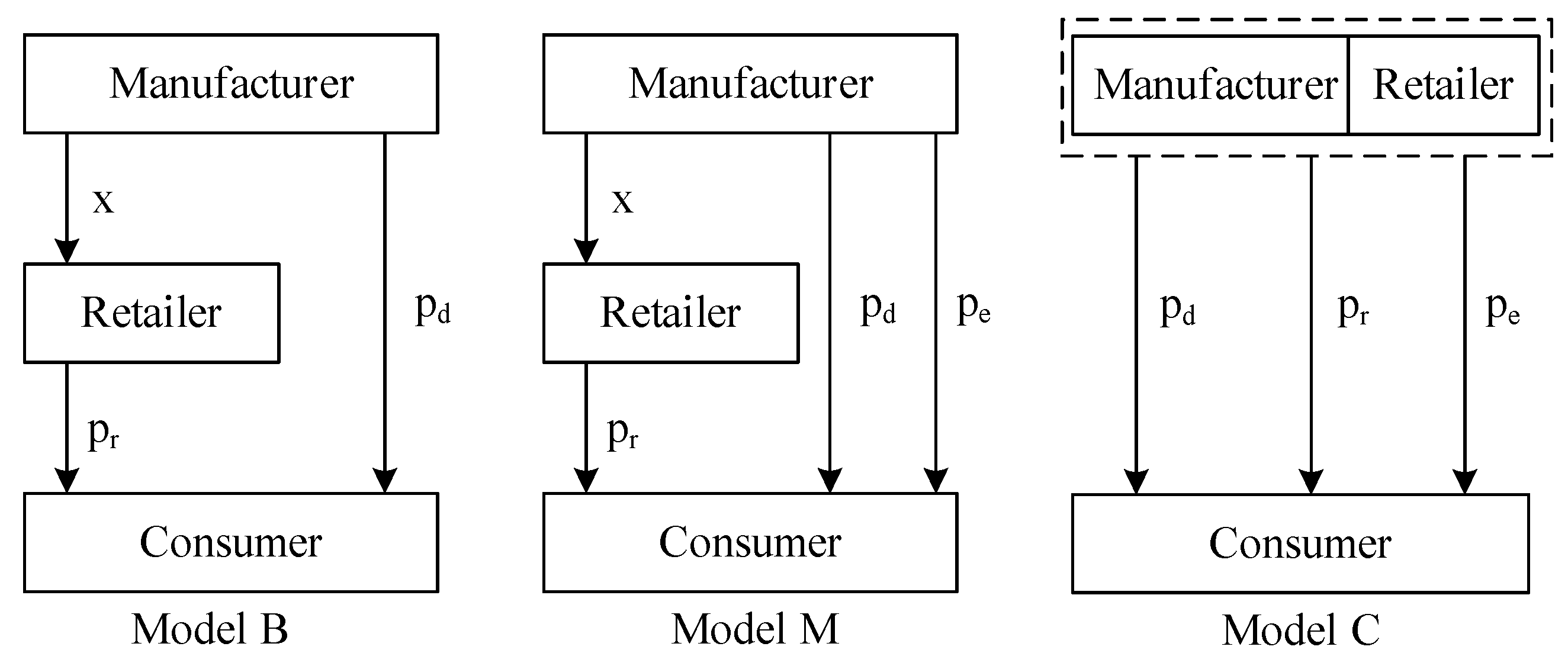
We consider a dual-channel supply chain with a manufacturer and a retailer. We first propose a basic decentralized decision model without the extended warranty (we call it Model B), then extend Model B to a decentralized decision model with the extended warranty (we call it Model M), and finally study a centralized decision model with the extended warranty (we call it Model C).
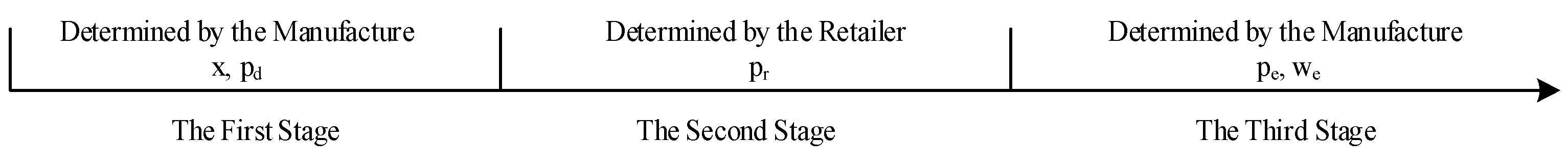
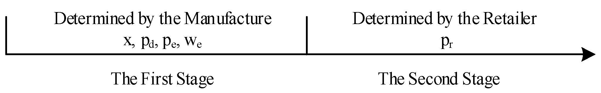
Figure 1 shows the structures of the three models. Note that, in Model M and Model C, the manufacturer sells the essential product through the retail channel, and meanwhile, sells the essential product as well as the extended warranty service through the direct sales channel. The extended warranty service can be treated as a separate commodity and is not bundled with the essential product. Consumers can choose to purchase only the essential product or both the essential product and the extended warranty service through the direct sales channel. In Model B and Model M, which are Stackelberg games, the manufacturer is the leader, and the retailer is the follower. We assume both the manufacturer and the retailer are perfectly rational and have symmetric information. We also assume the product demand is related to the product price only. Similar to the literature [
30,
31], the product demand of either the retail channel (
Dr) or the direct sales channel (
Dd) is defined as follows:
where
(
is the market size,
is the degree of consumers’ preference for the retail channel. As
θ increases, more consumers will choose the retail channel.
R (
is the cross-price effect, which reflects the degree of the price competition between channels.
is the consumers’ sensitivity to the product’s price. The manufacturer sells the extended warranty to the consumer at the price
. To facilitate the analysis and focus on the impact of the extended warranty only, let the base warranty of the essential product be zero.
Drawing from Bian et al. [
28], Panda et al. [
31], Heese [
32], and Jiang et al. [
33], we assume that there are two components of extended warranty costs. The first component is the unit maintenance and management cost
, which is linearly proportional to the length of the extended warranty period. The second component is the secondary cost
, which depends on the length of the warranty period. According to Li et al. [
34], the demand of the extended warranty is given as
where
. Throughout the paper, let the superscript “B” denote the basic decentralized decision model without the extended warranty, the superscript “M” denote the decentralized decision model with the extended warranty, and the superscript “C” denote the centralized decision model with the extended warranty.
5. Model Comparisons
5.1. Model B versus Model M
Let , , and . First, we note that there exists an equilibrium in Model M if and only if . In addition, to ensure and , we need and , respectively. Similarly, to ensure the optimal extended warranty period > 0, we need , which can be rewritten as .
Proposition 1. In the dual-channel supply chain, the extended warranty service provided by the manufacturer will lead to a lower price of the product in both channels, i.e.,
, but not affect the wholesale price, i.e., . The demand of the retail channel decreases and the demand of the direct sales channel increases after introducing the manufacturer’s extended warranty into the supply chain, i.e., and .(The attestation process is shown in the Appendix A). From Proposition 1, we know that when the manufacturer provides an extended warranty; in order to increase the sales of the product in the direct sales channel, he will decrease the price of the product in the direct sales channel. To compete with the manufacturer, the retailer also tends to decrease the price of the product; however, the wholesale price of the product offered by the manufacturer remains unchanged; therefore, the retailer does not have enough room to reduce the retail price, which finally causes a decrease in demand in the retail channel.
Proposition 2. Compared with Model B, the manufacturer and the whole supply chain would be better, i.e., and , but the retailer would be worse, i.e., in Model M. (The attestation process is shown in the Appendix A). Proposition 2 implies that when the manufacturer provides an extended warranty, his profit will increase, and the profit of the whole supply chain will increase as well; therefore, it is beneficial for the manufacturer to provide an extended warranty in the direct sales channel. However, the extended warranty will attract some consumers to transfer from the retail channel to the direct sales channel and make the retailer worse, which is not beneficial for the whole supply chain. Therefore, it is meaningful to find a way to achieve a win-win situation in the supply chain.
Proposition 3. In Model M, as (the consumer’s sensitivity to the price of the extended warranty) increases,
- (1)
both (the price of the product in the direct sales channel) and (the price of the product in the retail channel) increase, and (the price of the extended warranty) decreases;
- (2)
(extended warranty period) decreases;
- (3)
(demand of the product in the retail channel) increases, and both (the demand of the product in the direct sales channel) and (the demand of the extended warranty) decrease;
- (4)
( (the profit of the manufacturer) decreases, and (the profit of the retailer) increases. (The attestation process is shown in the
Appendix A).
Proposition 4. In Model M, as (the consumer’s sensitivity to the extended warranty period) increases,
- (1)
both
(the price of the product in the direct sales channel) and (the price of the product in the retail channel) decrease, and (the price of the extended warranty) increases;
- (2)
(extended warranty period) increases;
- (3)
(demand of the product in the retail channel) decreases, and both (the demand of the product in the direct sales channel) and (the demand of the extended warranty) increase;
- (4)
(profit of the manufacturer) increases, and (the profit of the retailer) decreases. (The attestation process is shown in the
Appendix A).
Proposition 3 implies that, in Model M, when consumers are more sensitive to the price of the extended warranty, the retailer will get more profits, but the manufacturer will lose more profits. On the contrary, Proposition 4 implies that, in Model M, when consumers are more sensitive to the extended warranty period, the manufacturer will get more profits, but the retailer will lose more profits. From both Proposition 3 and Proposition 4, we conclude that it is beneficial for the manufacturer to set a low price and a long period of extended warranty.
Proposition 5. In Model M, as either (repair cost per unit of time) or t (unit repair cost) increases,
- (1)
both (the price of the product in the direct sales channel) and (the price of the product in the retail channel) increase, and (the price of the extended warranty) decreases;
- (2)
(extended warranty period) decreases;
- (3)
(demand of the product in the retail channel) decreases, and both (demand of the product in the direct sales channel) and (demand of the extended warranty) decrease;
- (4)
(profit of the manufacturer) decreases, and (profit of the retailer) increases. (The attestation process is shown in the
Appendix A).
Proposition 5 shows that as the repair costs of the product increase, the manufacturer reduces the period of the extended warranty, and the demand for the extended warranty will decrease. In this case, to stimulate the demand for the extended warranty, the manufacturer will decrease the price of the extended warranty, and meanwhile, he will increase the price of the product to get extra income to compensate for the loss from the extended warranty. However, raising the price of the product in the direct sales channel will drive consumers to transfer to the retail channel from the direct sales channel, which leads to a decrease in the profit of the manufacturer, but an increase in the profit of the retailer.
5.2. Model M versus Model C
First, we also note that there exists an optimal solution in Model C if and only if .
Proposition 6. Comparing the optimal decisions in Model M and Model C, we have , , , and . (The attestation process is shown in the
Appendix A). Proposition 6 shows that, compared with the optimal decisions in the decentralized model (Model M), the price of the product in the direct sales channel increases, but prices of the product and the extended warranty decrease, and the period of the extended warranty also decreases, in the centralized model (Model C).
Proposition 7. Comparing realized demands in Model M and Model C, we have , , and . (The attestation process is shown in the
Appendix A). Proposition 7 shows that, compared with realized demands in the decentralized model (Model M), demands for the product and the extended warranty in the online direct channel decrease, but the demand for the product in the retail channel increases, in the centralized model (Model C).
Proposition 8. Comparing optimal profits in Model M and Model C, we have , where . (The attestation process is shown in the
Appendix A). Proposition 8 shows that, compared with optimal profits in the decentralized model (Model M), the whole supply chain always performs better in the centralized model (Model C). We also note that, in the decentralized model, thanks to the extended warranty, the direct sales channel has a great advantage over the retail channel; but in the centralized model, the retailer performs better than that in the decentralized model, the total profit of the whole supply chain is improved, and the supply chain reaches a win-win situation.
Proposition 9. In Model C, as (consumer’s sensitivity to the price of the extended warranty) increases,
- (1)
both (price of the product in the direct sales channel) and (price of the extended warranty) decreases;
- (2)
(extended warranty period) decreases;
- (3)
both (demand of the product in the direct sales channel) and (demand of the extended warranty) decrease, but (the demand of the product in the retail channel) increases;
- (4)
(total profit of the whole supply chain) decreases.
The impact of (the consumer’s sensitivity to the extended warranty period) on the realized demands, and optimal decisions and profits is on the opposite of the impact of . (The attestation process is shown in the
Appendix A). Proposition 9 shows that, in the centralized decision model (Model C), when consumers are more sensitive to the price of the extended warranty, the whole supply chain will lose more profits, and when consumers are more sensitive to the extended warranty period, the whole supply chain will get more profits. Therefore, it is beneficial for the supply chain to set a low price and a long period of extended warranty.
Proposition 10. In Model C, as either (repair cost per unit of time) or t (unit repair cost) increases,
- (1)
(price of the product in the direct sales channel) increases;
- (2)
(extended warranty period) decreases;
- (3)
(demand of the product in the retail channel) increases and (demand of the product in the direct sales channel) decreases;
- (4)
(total profit of the whole supply chain) decreases.
Especially, as increases, both (the price of the extended warranty) and (the demand of the extended warranty) increase, and the impact of t on and is on the opposite of the impact of . (The attestation process is shown in the
Appendix A). 6. Numerical Experiments
To study the impact of various model parameters on supply chain decisions, demands, and profits, we conduct some numerical experiments in this section. Based on the data presented in Zhang et al. [
30] and Panda et al. [
31], the default values of model parameters in numerical experiments are set as
,
,
,
,
, and
. These parameters ensure
and
to guarantee the optimal decisions and demands are larger than zero.
6.1. The Impact of Various Parameters on Optimal Decision and Demands
In this subsection, we analyze the impact of the consumer preferences , the price cross-elasticity coefficient of the product , and the price sensitivity coefficient of the extended warranty on optimal decisions and demands, in either the decentralized decision model or the centralized decision model.
- (1)
The impact of on optimal decisions and demands
When studying the consumer preference
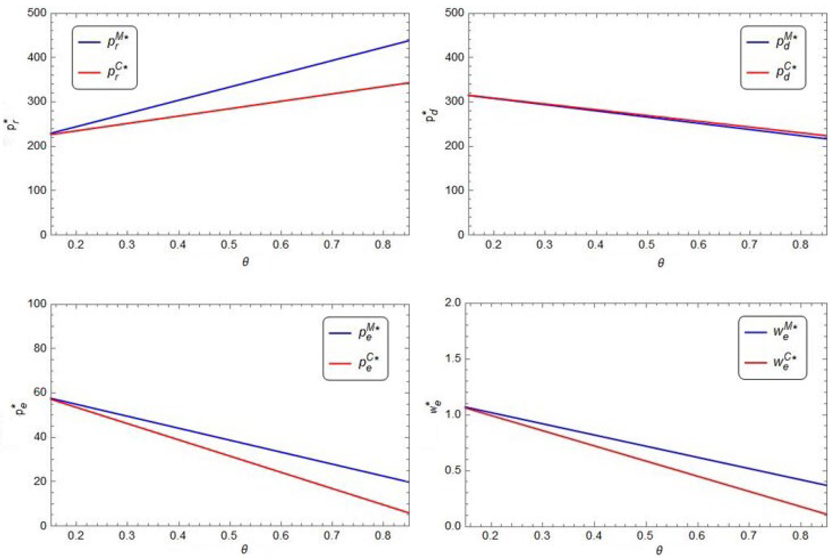
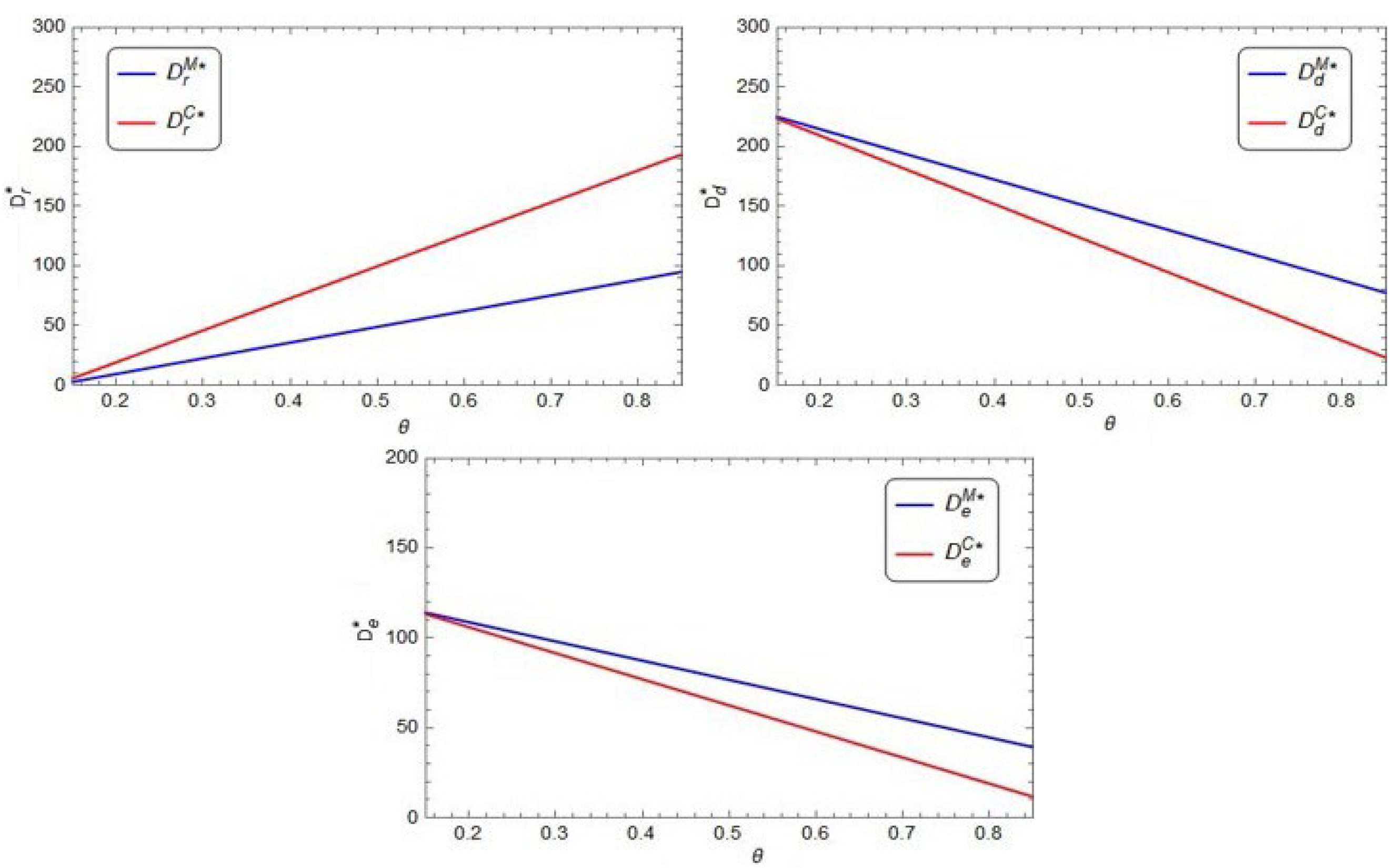
, we set its value range as [0.15, 0.85], and the specific data in the sensitivity analysis are shown in
Figure 4 and
Figure 5.
From
Figure 4, in both Model M and Model C, as the consumer preference
increases, the sales price of the product in the direct sales channel (
), the price of the extended warranty (
), or the period of the extended warranty (
) decreases, but the retail price of the product in the retail channel (
) increases. From
Figure 5, in both Model M and Model C, as
increases, the demand of the product in the retail channel (
) increases; however, the demand of either the product (
) or the extended warranty (
) decreases. It is observed that the consumer preference can make significant impact on the supply chain optimal decisions as well as the demands of either the product or the extended warranty. Compared to the decentralized supply chain; in general, the centralized supply chain is more sensitiver to the consumer preference. In addition, it is obvious that the retailer prefers high consumer preference for the retailer channel and the manufacturer is on the opposite.
- (2)
The impact of on optimal decisions and demands
When studying the price cross-elasticity coefficient of the product
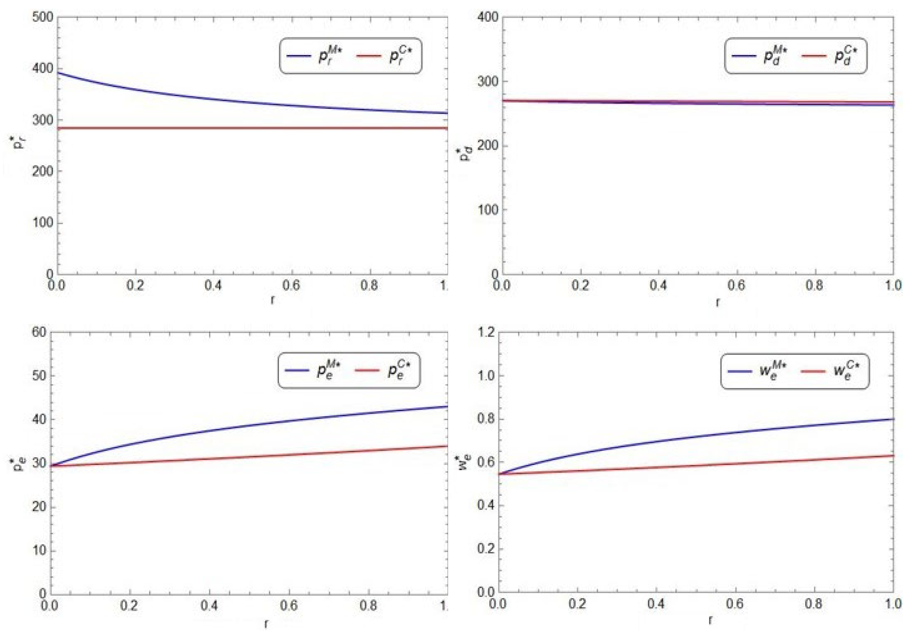
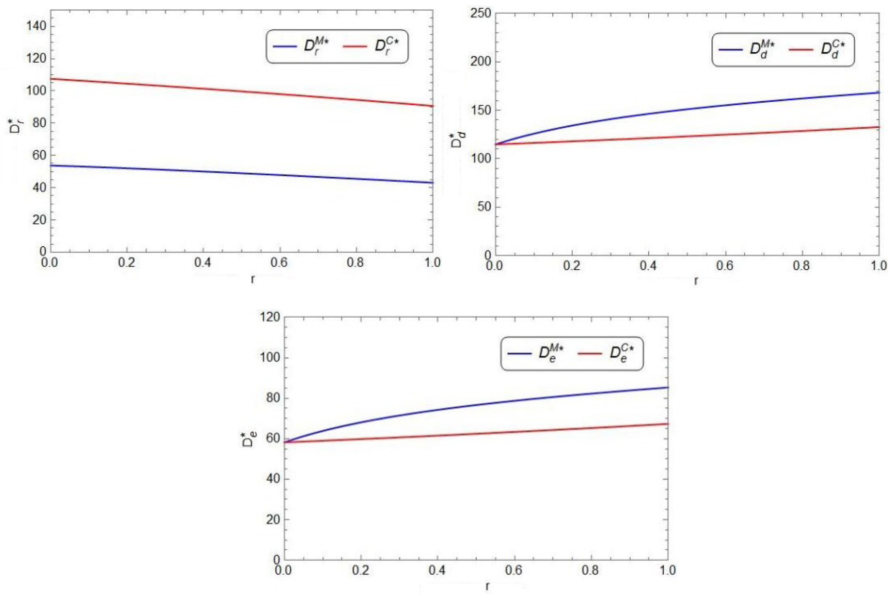
, we set its value range as [0, 1], and the specific data in the sensitivity analysis are shown in
Figure 6 and
Figure 7.
From
Figure 6, in both Model M and Model C, as the price cross-elasticity coefficient of the product
increases, the sales price of the product in the direct sales channel (
) slowly decreases, the price of the extended warranty (
), or the period of the extended warranty (
) increases. In addition, as
increases, retail price of the product in the retail channel (
) decreases in the decentralized supply chain but
remains unchanged in the centralized supply chain. From
Figure 7, in both Model M and Model C, as
increases, the demand of the product in the retail channel (
) decreases; however, the demand of either the product (
) or the extended warranty (
) increases. It is observed that the supply chain optimal decisions and the demands of either the product or the extended warranty are not very sensitive to the price elasticity, especially in the centralized supply chain. In addition, the retailer prefers low price elasticity, but the manufacturer is on the opposite.
- (3)
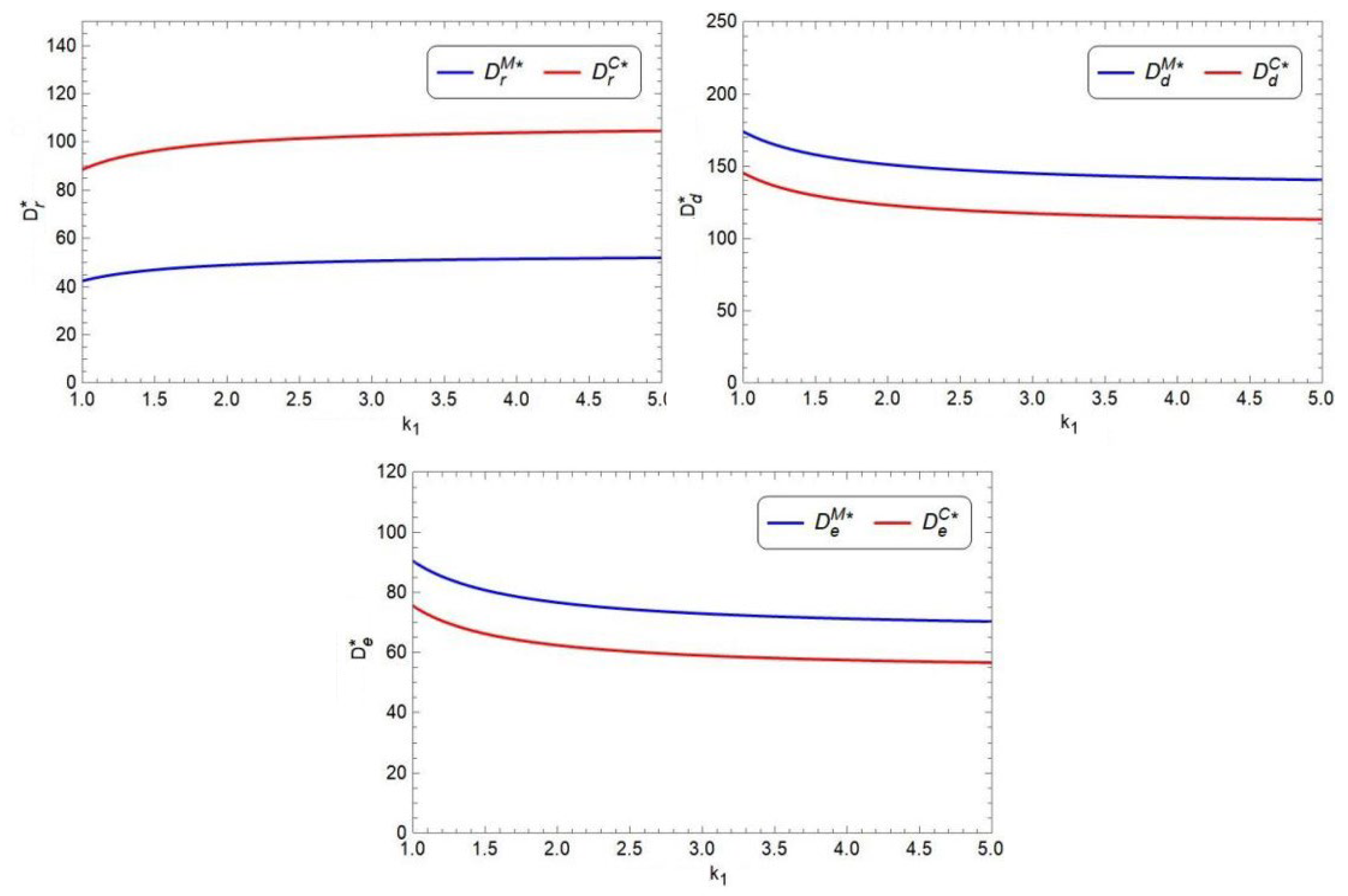
The impact of on optimal decisions and demands
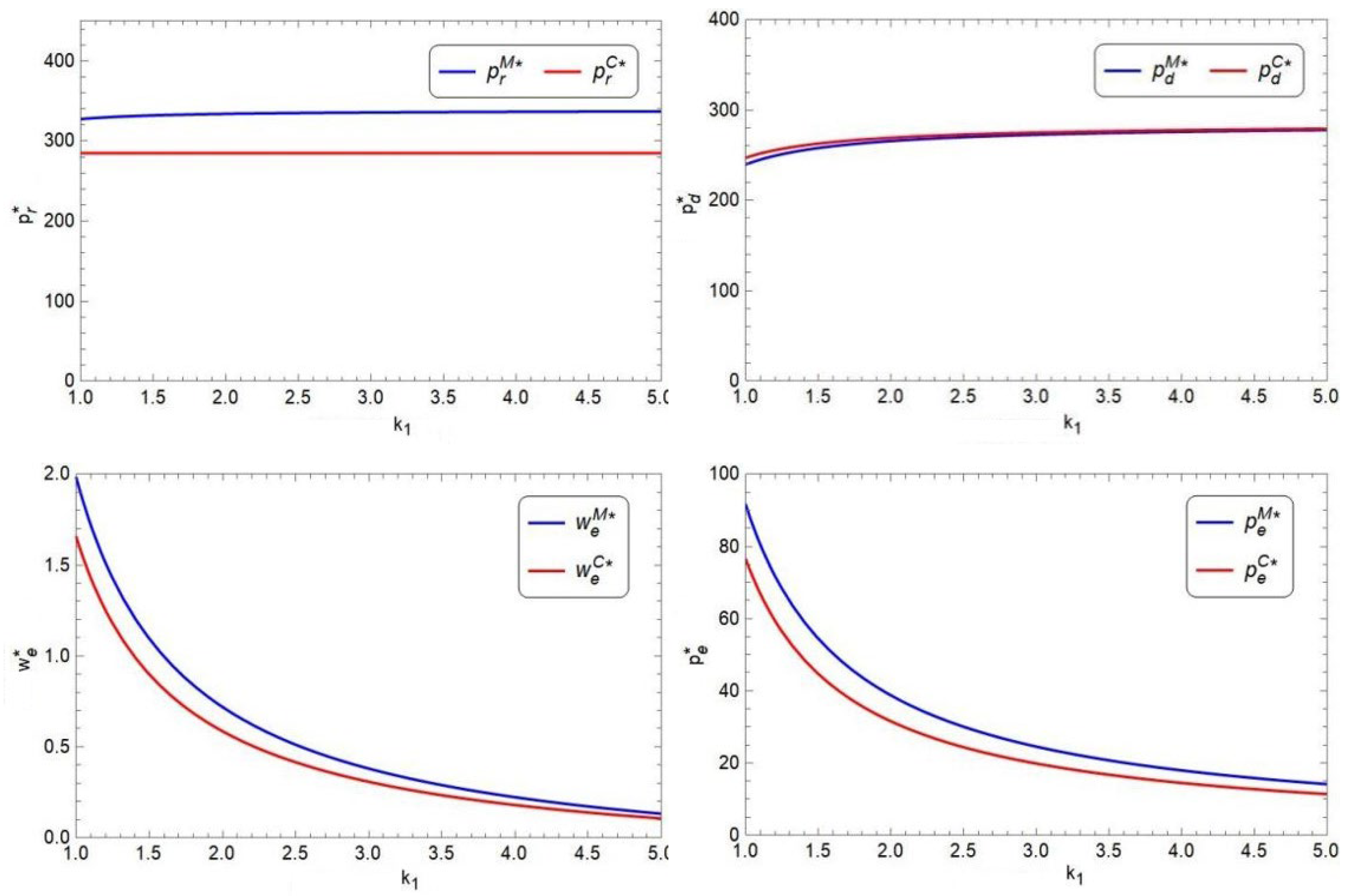
When studying the price sensitivity coefficient of the extended warranty
, we set its value range as [1, 5], and the specific data in the sensitivity analysis are shown in
Figure 8 and
Figure 9.
From
Figure 8, in both Model M and Model C, as the price sensitivity coefficient of the extended warranty
increases, the sales price of the product in the direct sales channel (
) slowly increases, the price of the extended warranty (
), or the period of the extended warranty (
) decreases. In addition, as
increases, the retail price of the product in the retail channel (
) slowly increases in the decentralized supply chain but
remains unchanged in the centralized supply chain. From
Figure 9, in both Model M and Model C, as
increases, the demand of the product in the retail channel (
) increases; however, the demand of either the product (
) or the extended warranty (
) decreases. It is observed that high price sensitivity of the extended warranty will lead to low price, short period, low demand of the extended warranty, and low demand of the product in the direct sales channel, but high demand of the product in the retail channel, and high product prices of both channels. Therefore, the retailer prefers high price sensitivity of the extended warranty, but the manufacturer is on the opposite.
Finally, from
Figure 4,
Figure 5,
Figure 6,
Figure 7,
Figure 8 and
Figure 9, we find that
set in Model C is always smaller than that set in Model M, and both
and
. set in Model C are also smaller than those set in Model M, but
set in Model C is always slightly larger than that set in Model M. Furthermore,
realized in Model C is larger than that in Model M, but either
or
realized in Model C is smaller than that in Model M. In general, compared with the decentralized supply chain, consumers can benefit more in the centralized supply chain.
6.2. The Impact of Various Parameters on Optimal Profits
In this subsection, we analyze the impact of the consumer preferences , the price cross-elasticity coefficient of the product , and the price sensitivity coefficient of the extended warranty on optimal profits of both the manufacturer and the retailer in either the decentralized decision model or the centralized decision model. Throughout this subsection, and represent the profit of the retailer and the manufacturer in the decentralized supply chain, respectively. and represent the profit of the decentralized supply chain and the centralized supply chain, respectively.
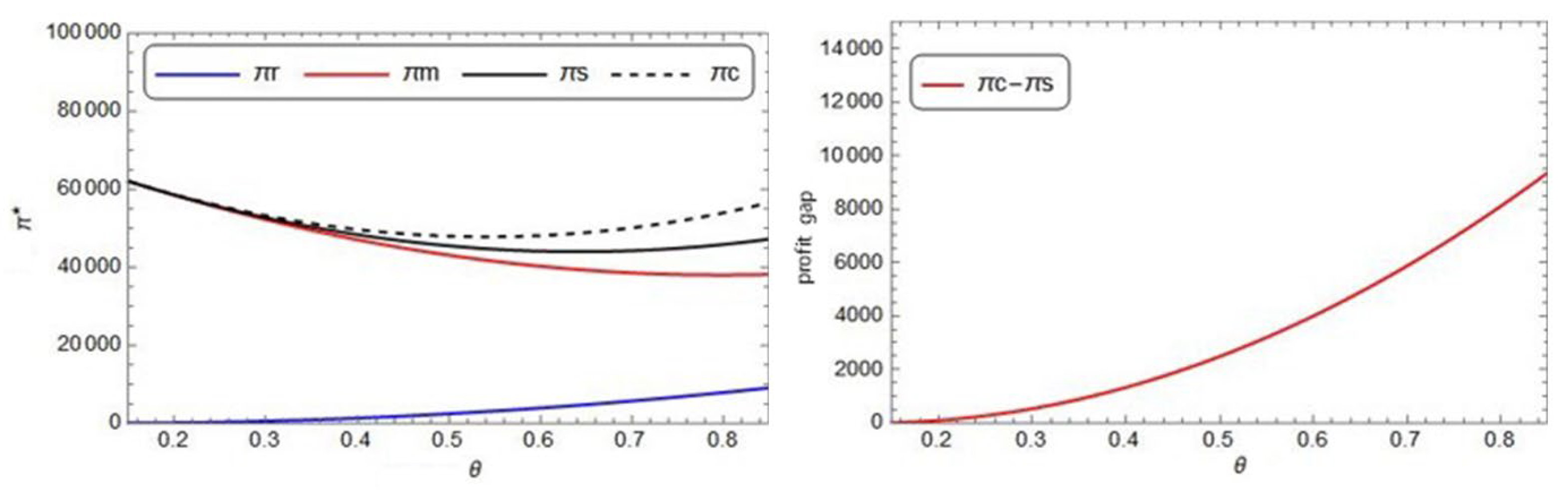
- (1)
The impact of on profits
The impact of
on
,
,
, and
is shown in
Figure 10 as follows.
From the left subfigure of
Figure 10, it is observed that as the consumer preference
increases, the profit of the retailer in the decentralized supply chain increases, but the profit of the manufacturer in the decentralized supply chain decreases, and the supply chain profit in either decentralized model or the centralized model first decreases and then increases. From the right subfigure of
Figure 10, it is obvious that the centralized supply chain always performs better than the decentralized supply chain when
varies over the interval [0.15, 0.85]. In addition, the extra profit of the supply chain brought by collaboration increases as
increases.
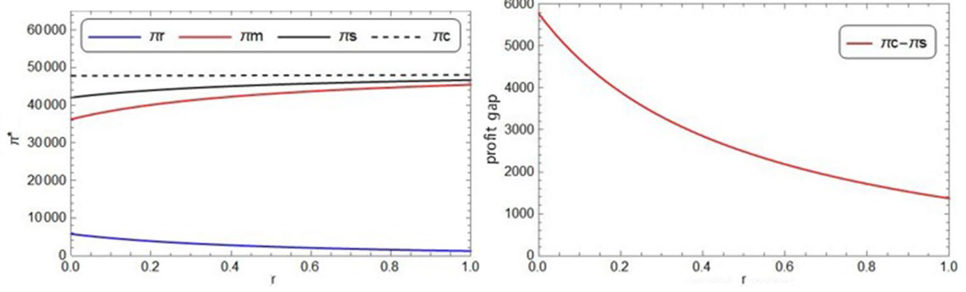
- (2)
The impact of on profits
The impact of
on
,
,
, and
is shown in
Figure 11 as follows.
From the left subfigure of
Figure 11, it is observed that as the price cross-elasticity coefficient of the product
increases. In the decentralized supply chain, the profit of the retailer decreases, but the profit of the manufacturer increases, and the whole supply chain profit increases; however, in the centralized supply chain, the whole supply chain profit always remains unchanged. From the right subfigure of
Figure 11, it is obvious that the centralized supply chain always performs better than the decentralized supply chain when
varies over the interval [0, 1]. In addition, the extra profit of the supply chain brought by collaboration decreases as
increases.
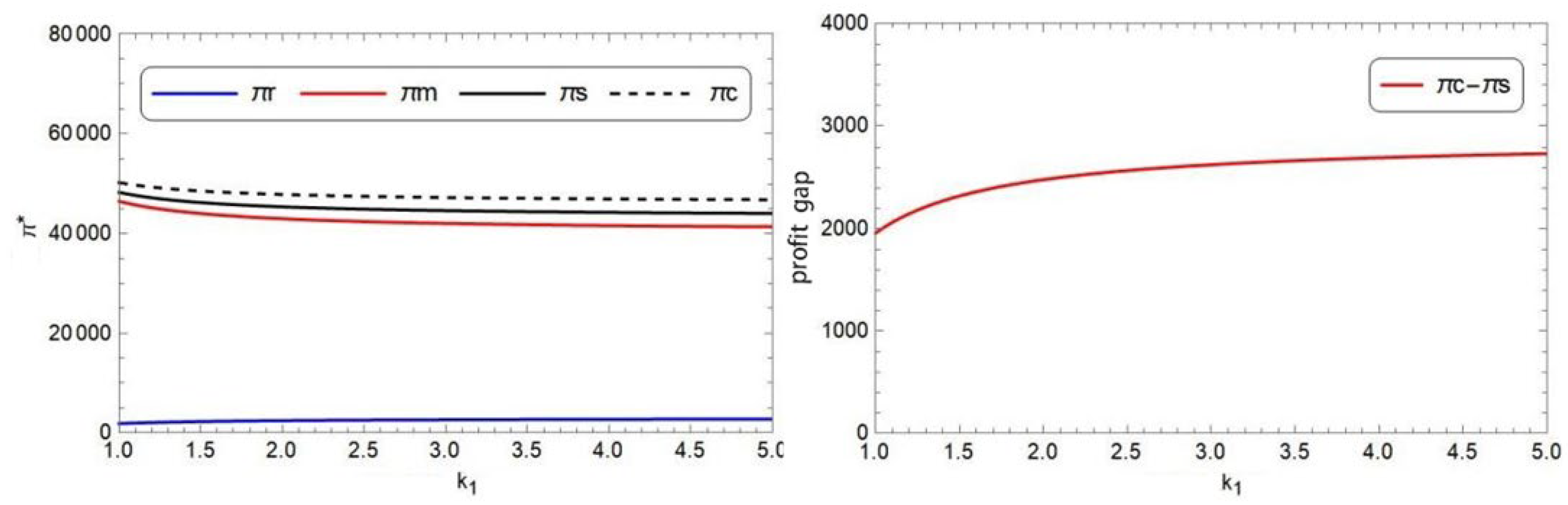
- (3)
The impact of on profits
The impact of
on
,
,
, and
is shown in
Figure 12 as follows.
From the left subfigure of
Figure 12, it is observed that as the price sensitivity coefficient of the extended warranty
increases, the profit of the retailer in the decentralized supply chain slightly increases, but the profit of the manufacturer in the decentralized supply chain slowly decreases, and the supply chain profit in either decentralized model or the centralized model also slowly decreases. From the right subfigure of
Figure 12, it is obvious that the centralized supply chain always performs better than the decentralized supply chain when
varies over the interval [1, 5]. In addition, the extra profit of the supply chain brought by collaboration increases as
increases.
Finally, from
Figure 10,
Figure 11 and
Figure 12, we find that the centralized supply chain always performs better than the decentralized supply chain. In addition, the retailer prefers high
and
, but low
, while the manufacturer is on the opposite.
In summary, the more consumers’ preference for retail channels, the greater the sensitivity of the prices, or the smaller cross-price elasticity between the two tracks; the manufacturer and retailers should strengthen cooperation to improve the supply chain’s total profit can effectively reduce losses. In addition, in the model set in this article, retailers are at an obvious disadvantage, which will cause the retailer market to continue to be squeezed and eventually withdraw from the market. Although the manufacturer has a competitive relationship with retailers, retailers are also a profit channel for manufacturers. Incredibly, multi-channel sales can increase their competitiveness with other products and have the advantage of incompetent online sales. Therefore, from the perspective of long-term profits and development, expelling retailers from the market is not wise.
7. Conclusions
We investigate a dual-channel supply chain with a manufacturer and a retailer and assume the extended warranty is provided by the manufacturer in the online direct channel. We build three models: (1) a basic decentralized supply chain model without an extended warranty (Model B); (2) a decentralized supply chain model with an extended warranty (Model M); a centralized supply chain model with an extended warranty (Model C). We optimize the three models and compare the optimal decisions and profits between Model B and Model M, as well as Model M and Model C. In summary, we have the following findings:
(1) Compared with Model B, prices of the product in both channels decrease, the demand for the retail channel also decreases, and the demand for the online direct channel increases in Model M; the manufacturer and the whole supply chain would be better, but the retailer would be worse, in Model M.
(2) Compared with Model M, the price of the product in the online direct channel increases, but prices of the product and the extended warranty decrease, and the period of the extended warranty also decreases, in Model C; demands of the product and the extended warranty in the online direct channel decrease, but the demand of the product in the retail channel increases, in Model C; the whole supply chain always performs better in Model C.
(3) Under centralized decision making, it always obtains higher profits than decentralized decision making; at the same time, it can be observed that the retail price of retailers in centralized decision making is lower and demand. The direct sales price set by manufacturers has mostly stayed the same. The time of extension and product demand is down; concentrated decision making retailers obtain benefits from it, while manufacturers have some benefits from the loss of part of the loss, but the overall profit increases.
(4) When consumers’ preference for retail channels and extended warranty price sensitivity continue to increase, the profit gap between the two decisions continues to grow. The profit difference between the two decisions decreases when the product cross-price elasticity coefficient increases. When A and B are larger or C is smaller, the larger the residual profit obtained by subtracting the decentralized decision making profit from the centralized decision making profit, the greater the amount of decentralized decision making profit loss.
According to these findings, we know that in the decentralized dual channel supply chain, providing an extended warranty in the online direct channel would benefit consumers, the manufacturer and the entire supply chain, but would harm the retailer. We also know that centralizing the supply chain will make the entire supply chain better off and achieve Pareto optimization of the supply chain system; however, although centralization would benefit the retailer and the entire supply chain, it would harm consumers and the manufacturer. Therefore, simply centralizing the supply chain is also not a good choice. To realize Pareto optimization of the supply chain and meanwhile achieve a win-win situation, the supply chain leader should try to find appropriate coordination contract mechanisms to resolve channel conflict and achieve cooperation between supply chain members, and finally realize a win-win situation and improve consumer welfare.
Although this paper has some conclusions and enlightenments, some limitations can be relaxed in the future to extend this paper and enrich the research on dual channel supply chain management with extended warranty services.
(1) This paper considers a dual channel supply chain model consisting of a single retailer and a single manufacturer with no horizontal competition. However, in the real world, the supply chain structure is much more complex, there is always competition, and the duopoly competition supply chain system and third-party competition are also important research directions.
(2) This paper assumes that the information for manufacturers and retailers is perfectly symmetrical. However, the research can be broadened to more general cases, such as supply chain members are information asymmetric, i.e., information held by manufacturers comes from direct channels, while the information contained by retailers comes from traditional markets.
(3) Besides analytical research on warranty services, we could further study warranty services in the dual-channel supply chain by using empirical methods in the future such as the SERVQUAL method used in Kadlubek, M, Jereb, B. [
35].


