Article

A Universality–Distinction Mechanism-Based Multi-Step Sales Forecasting for Sales Prediction and Inventory Optimization

1
School of Information Management, Sun Yat-Sen University, Guangzhou 510275, China
2
Information School, University of Sheffield, Sheffield S10 2TN, UK
*
Author to whom correspondence should be addressed.
Systems 2023, 11(6), 311; https://doi.org/10.3390/systems11060311
Submission received: 10 April 2023 / Revised: 12 June 2023 / Accepted: 14 June 2023 / Published: 19 June 2023

Abstract

:
Sales forecasting is a highly practical application of time series prediction. It is used to help enterprises identify and utilize information to reduce costs and maximize profits. For example, in numerous manufacturing enterprises, sales forecasting serves as a key indicator for inventory optimization and directly influences the level of cost savings. However, existing research methods mainly focus on detecting sequences and local correlations from multivariate time series (MTS), but seldom consider modeling the distinct information among the time series within MTS. The prediction accuracy of sales time series is significantly influenced by the dynamic and complex environment, so identifying the distinct signals between different time series within a sales MTS is more important. In order to extract more valuable information from sales series and to enhance the accuracy of sales prediction, we devised a universality–distinction mechanism (UDM) framework that can predict future multi-step sales. Universality represents the instinctive features of sequences and correlation patterns of sales with similar contexts. Distinction corresponds to the fluctuations in a specific time series due to complex or unobserved influencing factors. In the mechanism, a query-sparsity measurement (QSM)-based attention calculation method is proposed to improve the efficiency of the proposed model in processing large-scale sales MTS. In addition, to improve the specific decision-making scenario of inventory optimization and ensure stable accuracy in multi-step prediction, we use a joint Pin-DTW (Pinball loss and Dynamic Time Warping) loss function. Through experiments on the public Cainiao dataset, and via our cooperation with Galanz, we are able to demonstrate the effectiveness and practical value of the model. Compared with the best baseline, the improvements are 57.27%, 50.68%, and 35.26% on the Galanz dataset and 16.58%, 6.07%, and 5.27% on the Cainiao dataset, in terms of the MAE (Mean Absolute Error), MAPE (Mean Absolute Percentage Error), and RMSE (Root Mean Squared Error).

1. Introduction

Sales forecasting is an area of research with considerable practical significance due to its potential to improve commercial decision-making. However, the influences of external observable and unobservable factors, e.g., the weather, seasonal promotions, adjustments in sales strategies, etc., make forecasting particularly challenging. Such factors cause irregular fluctuations in sales, resulting in large deviations in sales forecasts. In many circumstances, even a slight reduction in such deviations can bring great benefits. For example, the optimization of sales forecasting for high-profit commodities can greatly reduce losses in profit caused by stock shortages. A second area in which there is scope for development, and where there appear to have been few studies, is that of specific enterprise decision-making scenarios, such as inventory optimization. In Galanz’s e-commerce business scenario, the average profit per unit of goods surpasses its inventory management cost. As a result, shortages lead to greater losses than excess inventory, which means that, with the same sales prediction deviation, predicting less than the actual sales may lead to greater losses than predicting more, which is one of the challenges of sales forecasting.
The problem of dealing with complex and diverse influencing factors is generally addressed by using a multi-step time series prediction based on multivariate time series (MTS). The specific models can be divided into traditional time series prediction methods and deep learning models. Figure 1 shows an actual sales sequence, together with the results of multi-step time series predictions made using, respectively, deep learning models (MLCNN [1]) and traditional methods (ES [2]). Both predictions deviate considerably from actual values when there are sudden peaks in sales.
Existing research has proven that deep networks are capable of capturing valuable implicit information, and can be effective in predicting abnormal fluctuations in sales sequences. In the M4 time series forecasting competition, the winning method, [3], adopted a hybrid hierarchical prediction scheme, incorporating the standard exponential smoothing model (ES) into a common framework with long short-term memory (LSTM) networks; this approach resulted in better performance compared to traditional and machine learning methods. Traditional time series analysis methods and machine learning models, such as the autoregressive model (AR) [4], moving average (MA) [5], random forest (RF) [6], and XGBoost (XGB) [7], are widely used in sales forecasting. However, these methods are difficult to use when modeling large-scale MTS. For example, more than 10,000 time series need to be considered at the same time in traffic MTS prediction tasks. Sales forecasting is another complex and computationally intensive MTS task. It needs to consider various factors, including price, preferential strategy, and the sales of related commodities. The accuracy of these methods in capturing nonlinear correlation patterns needs to be improved. As is obvious from Figure 1, the exponential smoothing (ES) model fails to predict the nonlinear changes in a real sales sequence, leading to the accumulation of errors in the multi-step prediction. To some extent, deep learning models can solve the problems that traditional machine learning methods have with MTS prediction. They can fit each sequence independently and share general rules for different sequences. LSTNet [8] makes use of the advantages of CNN(Convolutional Neural Networks) and RNN(Recurrent Neural Networks) to capture the dependency patterns associated with different periods and it shares knowledge in multivariate time series (MTS). Deep learning models are also capable of automatically extracting features to reduce the work of artificial design features. Temporal fusion transformers [9] can automatically select relevant features and suppress unnecessary ones through a series of gating layers. Moreover, deep models improve the efficiency of dealing with long-period and large-scale MTS data [10].
Previous studies that applied deep learning models to fields such as traffic, finance, and industrial production, have shown promise, but there are deviations in the multi-step sales forecasting tasks. Consequently, deep learning is a key research direction for MTS prediction and is the focus of this paper. However, as is evident from Figure 1, although the deep learning model is more effective at capturing fluctuations than the ES model, it does not accurately predict sudden large fluctuations, which is the first challenge in our research. Ad hoc marketing strategies or other unforeseen factors can lead to unusual fluctuations in sales series. Furthermore, compared to other time series forecasting tasks, such as transportation and finance, one main difference is that sales time series are more susceptible to external uncertainties that can dynamically alter the internal correlations between sales time series. These external uncertainties are critical factors that cannot be predetermined or observed in advance and may result from various causes, such as product reviews on social media, regional promotions, and the introduction of new competitive products. The differences were further verified in previous studies [1,10,11,12]. Deep learning models used to predict public MTS, such as transportation, energy, exchange rates, etc., often obtain good performances, and the improvements brought about by the new models are limited. The reason for this is that public MTS data exhibit more pronounced correlation patterns compared to sales time series, and these patterns are less influenced by external changes. Thus, the future trends of those MTS could be predicted more easily than those of sales time series.
Currently, few sales forecasting studies are based on specific decision-making scenarios. This is particularly important because the general model may not be directly applicable to specific scenarios, mainly due to issues such as mismatched decision objectives. Specific decision-making scenarios entail more constraints in mathematical expressions. This paper exemplifies the decision-making scenario of inventory optimization and emphasizes the integration of constraints into the deep learning model to achieve end-to-end efficient training and application. As mentioned above, one of the main targets of inventory optimization is to design a constraint that makes the predicted sales greater than the true sales, on the premise of minimizing prediction errors as much as possible, thereby reducing shortage risks. Modeling this constraint is the second challenge of our research since it requires finding an optimal balance between inventory shortages and excesses, considering time delays and abnormal fluctuations.
The two challenges mentioned above not only have theoretical values but also have practical values, which are essential in sales prediction. Many complex and changeable variables in the market will significantly influence the prediction results for products. For example, various online promotional activities will have huge impacts on sales fluctuations. Some products with dozens of daily sales may reach thousands of sales in one day due to temporary promotional activities. Of course, there are also many goods that are not sensitive to price fluctuations and are not significantly affected by external factors. This will make solving the target problem that is to be predicted more complex. Therefore, it is necessary to model and analyze the unique characteristics of each time series separately to better understand the fluctuation patterns of each time series. Due to the impact of fluctuations, there may be a significant deviation between the predicted sales and the true sales. This deviation can result in additional operational or cost losses in different decision-making scenarios. In the inventory optimization scenario, assume that, at time t, the task is to predict the sales at time t + 1. When the predicted sales at time t + 1 are much lower than the true value, the problem is even more serious because the enterprise will bear the losses caused by the inventory shortage. The inventory loss can be calculated as the product price × |true sales − predicted sales| at time t + 1. Thereby, solving these two challenges is essential for enterprise decision-making, especially in the domain of inventory optimization. The improvement in sales prediction could help top manufacturing enterprises in saving hundreds of millions of dollars in average annual inventory costs.
To summarize, in the multi-step prediction of MTS, existing research methods are not adept at capturing non-linear changes or accurately predicting sudden fluctuations. This is because the current research mainly focuses on extracting sequence correlations between time series in an MTS, while seldom considering the differences between time series. To solve these problems, we designed a universality–distinction mechanism framework, which independently models the universality and distinction of the sales sequence. First, the universality mechanism can extract instinct features and common correlation patterns with a similar context from MTS. The instinct features are unique characteristics of each commodity, such as the sales range level and the distribution of sales numbers. Common correlation patterns within a similar context signify the general association between different types of time series, such as the correlations between the sales of a specific commodity and its promotional activities during a given time. Second, ad hoc marketing strategies or other unforeseen factors can lead to unusual fluctuations in sales series. A manual inventory strategy will incorporate the analyses of historical sales and current market conditions to formulate or adjust inventory plans. We devised a distinction extraction module that simulates manual inventory strategies to capture the sales fluctuations caused by these unexpected factors. The red box shown in Figure 1 is the prediction window and clearly shows the effects of existing models on predicting sudden high sales. The yellow box is part of a historical sales series that experienced similar fluctuations to those in the red box. The distinction extraction module captures the unique characteristics of a specific time series from its similar sub-sequences (ex: two windows in Figure 1) and improves the prediction of sudden fluctuations. By modeling the universality and distinction independently, the impacts of large fluctuations can be reduced and the deviations in the prediction of abnormal fluctuations can be minimized.
In addition, although the proposed universality and distinction mechanism can obtain more accurate representations of common and different data from time series in an MTS, we need to design an optimal loss function to adopt the information that was extracted for better sales predictions in a complex environment, such as the issues of shape distortion and time delays in multi-step forecasting. More importantly, the purpose of sales prediction is to realize inventory optimization. According to the investigation results, the cost of shortages is higher than the cost of excess inventory under the same conditions. Considering the characteristics of commodity inventory costs, as well as the issues of shape distortion and time delay in multi-step forecasting, we developed a loss function called Pin-DTW to improve predictive performance.
The main innovations of the model presented in this article are as follows.
  • We propose a universality–distinction mechanism (UDM) framework, which consists of universality extraction and distinction-capturing components to improve the accuracy of predictions of multiple future steps.
  • “Universality” refers to the inherent characteristics and common correlation patterns found in sales sequences with similar contexts. The shared knowledge is initially learned through a universality extraction component that ensures the overall prediction window’s accuracy.
  • “Distinction” refers to the process of identifying differences between time series in a sales MTS. To achieve this more efficiently, we propose an attention-based encoder–decoder framework with query-sparsity measurements, which enables us to capture distinct signals based on the states of future multi-step sales.
  • We developed a novel loss function called Pin-DTW by jointly combining the pinball and DTW losses to enhance predictive performance. The DTW loss can make better use of the representations obtained from UDM to handle issues of time delay and shape distortion in future multi-step predictions. The pinball loss can be used to control the inventory shortage risk.
The purpose of our research was to design an end-to-end component that integrates a deep learning model and considers a specific decision-making scenario, which can be easily inserted into existing sales forecasting models or frameworks. This has the potential benefit of improving the overall prediction performance of the model in nonlinear relationship discovery and informing specific decision-making scenarios, resulting in cost savings and improved efficiency for enterprise production and sales. An example of our cooperation with Galanz is described in detail in the experiments section. The source code and data are available at https://github.com/lx237/2023UDM (accessed on 11 February 2023).

2. Related Work

2.1. Time Series Prediction

Time series prediction involves a wide range of fields, including inventory management [13], macroeconomic forecast [14], natural phenomena observations [15], and medical and industrial detection [16]. Highly structured data have strong and complex dependencies among different time steps, and it is a great challenge to effectively model the complex dependencies. The VAE(Variational Auto-Encoder) provides flexible nonlinear mapping and effective inference capabilities [16]; it has been proposed that the VAE can be extended as a recurrent framework to model high-dimensional sequences. Aiming to predict sparse multivariate sequences, [17], a dynamic Gaussian-mixture-based deep generative model was devised, which can model the transitions of latent clusters of temporal features and the emissions of MTS using dynamic Gaussian mixture distributions. From the perspective of time series representation [18], a contrastive learning framework named TS-TCC(Time-Series representation learning framework via Temporal and Contextual Contrasting) was proposed. TS-TCC creates two views by applying strong and weak augmentations to learn robust representations of time series. Experiments have demonstrated the effectiveness of the TS-TCC framework for time series prediction, classification, and other downstream tasks.
Long sequence prediction is also a challenge in time series prediction, where the model is required to accurately capture the long-term dependencies between the input and output. Traditional time series analysis methods, such as the well-known autoregressive moving average (ARMA) and its variants, have proven to be effective in various real-world applications, but they cannot model nonlinear relationships. Yao Q et al. proposed a dual-stage attention-based recurrent neural network (DA-RNN) that can properly capture long-term dependencies and select relevant driving sequences to make predictions [11]. In addition, the informer, which is based on the transformer, can effectively capture the dependencies in long sequences. This enhances the capability for long time series prediction and effectively controls the time and space complexity of model training. The generative informer decoder can also avoid the diffusion of cumulative errors [10]. Farnoosh et al. proposed deep switching autoregressive factorization (DSARF), a deep generative model designed for spatiotemporal data; it has the ability to unravel recurring patterns in the data and perform robust short-term and long-term predictions [12].
Existing work generally reveals the potential trends and patterns from the perspective of time and features, but the efficiency of these models is not always sufficiently explained. A novel strategy called series saliency [19] was proposed for time series analysis and prediction, considering both accuracy and interpretability.

2.2. Sales Forecasting

Sales forecasting is an application that involves time series prediction, which is of practical significance and value to enterprises. In practical research, sales are related to many factors, such as marketing strategies, the weather, and holidays, the complexity of which determines the difficulty of sales forecasting. Aiming to fully capture the dynamic dependencies among multiple influential factors [20], a novel framework for sales prediction named TADA +  was proposed, which is enhanced by an online learning module used to carry out trend alignment with dual-attention and multitask RNNs. This is one application of deep learning models, and there are other types of predicting methods, which are classified as follows:

2.2.1. Machine Learning Methods

Hirche et al. [21] used weighted random forest (WRF) to predict under- and over-performing consumer-packaged goods of retail stores, including convenience stores, drugstores, food stores, liquor stores, and mass merchandise retail stores. Forecasting future sales changes in products holds great significance for retailing companies. Machine learning models and traditional time series models were both employed to analyze and predict Walmart sales, and the experiments showed that the former performed better [22]. Machine learning methods are widely used in measuring market performance for retail stores, and are also essential in facilitating the transformation from a traditional offline sales model to the B2C model. Brick-and-mortar retail has been hit harder than ever by the COVID-19 pandemic. In [23], the authors achieved this transformation by building a purchase prediction model with XGBoost and random forest. Accurately predicting sales is of high importance to improve the effectiveness of the supply chain. In inventory management, machine learning models, such as RF, XGB, and LGBM models, are used to extract knowledge from large amounts of historical data to predict future orders [24].

2.2.2. Deep Learning Models

Existing studies have applied deep learning models to sales forecast tasks. Reference [25] compares the performances of some deep learning models, including simple RNN, LSTM networks, bidirectional LSTM networks, encoder–decoder LSTM networks, and CNN, in the multi-step time series prediction task, and the bidirectional and encoder–decoder LSTM network provided the best performance in terms of accuracy. Reference [26] proved the effectiveness and robustness of LSTM in comparison to FF-recursive and FF-multi-output models in the multi-step prediction of noise-free, chaotic time series. Reference [27] collected and preprocessed the historical sales volumes and multi-channel online sentiment data to forecast the movement direction of car sales in Taiwan with a CNN-LSTM model. As one of the classic deep learning models, LSTM performed well in terms of advertising expenditures, sales, and demand forecasting [28]. Reference [29] used a deep learning method to predict new product sales in the fashion industry, which was compared with the linear regression, random forest, SVR(Support Vector Regression), and ANN(Artificial Neuronal Networks) models, and the evaluation results show that the deep learning model was no better than the use of single models (such as random forest). Reference [30] proposed a new deep neural framework for e-commerce sales prediction, named DSF(a novel deep neural framework for sales forecasting), which was applied to the Alibaba e-commerce dataset. DSF uses five kinds of features related to sales, including static and dynamic features (such as user behavior characteristics and promotional activities), to forecast sales, which can explicitly simulate the influence of competitive relations and improve model performance.

2.2.3. Integrated Models
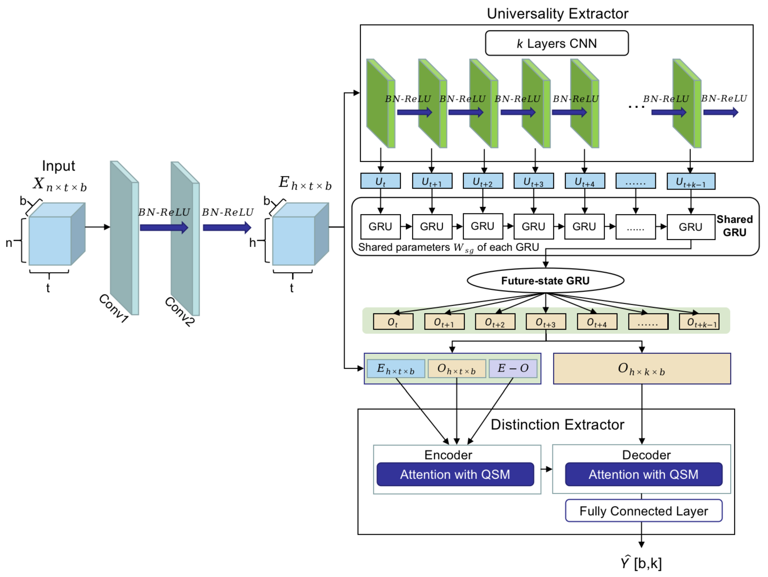
Reference [31] put forward a meta-learning framework based on a dual-channel convolution neural network (DCCNN), which automatically learns feature representation in original time series data, and then links the feature representation with a set of weights. The weights are used in basic model combinations, such as random forest and GBRT, and finally find the best combination. A hybrid method composed of a linear model (ARIMA) and a non-linear model (LSTM) was employed to calculate a monthly sales quantity budget based on an enterprise’s previous income data [32]. In the demand forecasting task for multi-channel fashion retailers [33], an integrated approach combining k-means clustering, extreme learning machines, and support vector regression was utilized to address challenges caused by the lack of historical data and product demand uncertainty.
Existing research has succeeded in the multi-step prediction of MTS and sales forecasting. However, research has mainly focused on modeling the correlation patterns between time series, and seldom considered how to model and capture the nonlinear dynamic changeable patterns and distinct fluctuation signals. In this research, we designed a universality–distinction mechanism framework to solve these problems to a certain extent. The universality extraction is used to capture linear and non-linear correlation patterns from the MTS, and distinction capturing can capture distinct fluctuation signals of each time series based on the extracted correlation patterns.

3. Model

This section describes the proposed universality–distinction mechanism (UDM) framework in detail. UDM is a mechanism proposed to improve the performance of future sales predictions. According to previous studies [34,35] and the practical operating methods of e-commerce and manufacturing enterprises, inventory optimization is an objective of sales forecasting. Thus, in order to better optimize inventory, we firstly need to accurately predict future sales. The sales value predicted in this study is very important and is used as a reference for the minimum inventory level, which is provided for marketers to determine the final inventory level, in combination with marketing plans. As shown in Figure 2, first, the UDM framework starts with a convolutional component to encode the multivariate sales sequence and map the input to a higher dimension space. Then, the encoded sequence will be fed into a universality-extracting component to extract common knowledge. Next, the distinction-capture module is used to identify the differences between different prediction steps. Finally, the vector representations that consider the universality and distinctions are mapped to a one-dimensional space as the final output result. In addition, in order to ensure the accuracy and stability of the model, we devised a Pin-DTW loss function to minimize the shape and time delay loss by considering inventory shortage risks. We will introduce each component of our architecture and the loss function in the following subsections.

3.1. Problem Statement

Assume that there are N products  X = { X 1 , , X i , , X N }  of different models in a warehouse. The sales time series of the ith product  X i = X n × t i  through timespan  1 t  has n features. Features include the product type, shop discount, and discount rate. The main aim of this research is to predict the sales  Y t + 1 t + k  of all N products at time  t + 1 t + k , where  Y t + 1 = { Y t + 1 1 , , Y t + 1 N }. The objective function can be described as follows:  Y ^ t + 1 = U D M ( X 1 t 1 N ) X 1 t 1 N  are divided into many batches, and each batch  X n × t × b  (n is the number of features, t is the length of the historical sales sequence, and b is the batch size) is individually input into the UDM. The input  X n × t × b  is first encoded by a convolution component, and the output is  E h × t × b . The output is then fed into a universality-extracting component to extract common correlation patterns  O h × t × b  and generate features  O h × k × b  that fuse future information for the final predictive task. Based on the encoded original input  E h × t × b  and the common correlation patterns  O h × t × b , we can obtain the matrix  Z h × t × b  with distinct fluctuation signals. These three matrices are mainly used to generate the final predictions  Y ^ b × k  through an efficient attention mechanism in distinction capturing. Here,  f E  and  f D  refer to the encoder function with the self-attention mechanism and the decoder function with cross-attention mechanism, respectively. The prediction  Y ^ b × k  represents the future k-step predicted values in a batch. Assuming that the real sales are from time  t + 1 t + k  is  Y t + 1 Y t + k ;  the target of the prediction task is to minimize the deviation between these two sequences. We use a joint  L P i n D T W  loss function, which consists of  L P i n  and  L D T W  to prevent a greater out-of-stock cost and align the ground-truth sequence and predicted value sequence. Some important variables and their explanations are listed in Table 1.

3.2. Convolutional Component

For the input time series (TS)  X n × t × b , we adopted a two-layer convolutional network with batch normalization and  R e L U  activation functions, as shown in Figure 2, as the first part of UDM. For each filter, the kernel size is  1 × 1 . Batch normalization helps to accelerate network convergence, and we assigned the  R e L U  activation function to add nonlinear factors to improve the network’s expression ability. This convolutional component is used to increase the input dimension and information interactions between different features. The input  X n × t × b  is encoded by the component as  E h × t × b (h is the hidden size):
E h × t × b = R e L U ( B N ( C o n v 2 ( C o n v 1 ( X n × t × b ) ) ) ) ,
where the  R e L U  function is  R e L U ( x ) = m a x ( 0 , x )  and the encoded sequences  E h × t × b  are high-dimensional vectors with latent representations and abstract information.

3.3. Universality Extracting

The encoded sequences  E h × t × b  are fed into a universality-extracting component, which is a component used to extract the common temporal features and local correlation patterns and generate construals of multiple future k time steps. This module contains k layers, a convolutional neural network (CNN), a shared GRU, and a future-state GRU, which are described as follows. First, at the i-th CNN layer, where  i k , the CNN model is used to capture the local correlation patterns of the MTS at a future time step  t + i , based on the correlation patterns captured from time  t + i 1 . The correlation patterns can be seen as the construals of future k predictive steps, and are regarded as having a relatively universal law to describe non-linear correlations between different time series within MTS. In our model, we constructed seven different construals for seven predictive steps using a seven-layer CNN:
U t = Ψ 1 ( E h × t × b ) , U t + 1 = Ψ 2 ( U t ) , U t + k 1 = Ψ k ( U t + k 2 ) ,
where  E h × t × b  is the matrix of the encoded sequence.  Ψ i , i [ 0 , k ]  are one-dimensional convolutional layers (Conv1D), where the kernel size is 3, stride is 1, and padding is 1. After the convolution operation, we apply the LeakyReLU function as an activation function. Moreover, we use the dropout operation to avoid overfitting.  U t , U t + 1 , , U t + i , U t + k 1  are the construals extracted by the multi-layer CNNs described above.

3.3.1. Shared GRU

The construals  U t , U t + 1 , , U t + k 1  derived from CNNs of different steps are then individually fed into a shared GRU to share information and model the relations among multiple predictive steps. Similar to MLCNN [1], the shared component learns the states of MTS at a future time step  t + i , where  i k , based on the correlations between different times in  U t + i ; the formula could be described as follows:
For i in range ( 0 , k ) O h × t × b = shared GRU ( U t + i , O h × t × b | W s g ) , Y ^ t + i , b = f L ( O h × t × b ) ,
where  O h × t × b  is the sequence correlation representations of the MTS from time 0 to t in a batch b, and the length of the hidden state of the representation is h. The shared GRU is mainly based on a gated recurrent unit (GRU) component [36], which can model the sequence correlation-based hidden state  O [ h , t , b ]  in  O h × t × b  at a different time  t , where  t t . Shared GRU has two parameters: the first parameter  U t + i  is the local correlation matrix, which is related to the value at a future time step  t + i . The second parameter  O h × t × b  indicates that the sequence correlation-based hidden states for a future time step  t + i  accumulate based on the  O h × t × b  at time  t + i 1  (in equation (3), the “For” loop is used to realize the accumulation).  W s g  is the set of shared weights of the GRU component. For each GRU,  Y ^ t + i , b  will be predicted based on the shared parameters  W s g , and the predicted value will be used to update the  W s g , which will be taken as the initial parameters for the next GRU with the input as  U t + i + 1 . For the  t th hidden state  O h , t , b  of GRU, the formula could be described as follows:
O [ h , t , b ] = GRU ( O [ h , t 1 , b ] , U t + i ( : , t ) ) ,
where GRU is the recurrent unit of the GRU component;  O [ h , t , b ]  is the  t th sequence correlation-based hidden state of tensor  O h × t × b , and the length of the hidden state is h U t + i ( : , t )  represents the  t th column of  U t + i ; this is used to represent the local correlations at a time point  t , and the local correlations will have a significant influence on the value in a future time step  t + i . The formula indicates that the hidden state  O [ h , t , b ]  is determined by its previous hidden state and the  t th column of  U t + i .

3.3.2. Future-State GRU

The future-state GRU is designed to use each local correlation matrix  U t + i , where  i k  represents the future sequence correlation-based hidden state at each future time step  t + i . Its main purpose is to obtain the initial representations at each future time step by integrating knowledge of instinct features and common correlation patterns from different construals. For example, many sales of a commodity at a future time step  t + i  have a high probability of being correlated with the average sales number, which ranges from time 0 to t; this could be regarded as an intrinsic feature of the commodity. As introduced in the previous section, the construals are the set of local correlation matrices:  U t + i  ( U t + i  has t rows; the  t th row can be seen as the representation of the local correlation patterns between time series at time  t ), which is provided for all predictive steps to learn the universality of future steps. Assume that at time  t + i , the hidden state of the future-state GRU at time  t + i  is computed as follows:
z t + i = σ ( W z · [ O t + i 1 , U t + i ] ) , r t + i = σ ( W r · [ O t + i 1 , U t + i ] ) , O ^ t + i = tanh ( W · [ r t + i O t + i 1 , U t + i ] ) , O t + i = ( 1 z t + i ) O t + i 1 + z t + i O ^ t + i .
where ∗ indicates Hadamard product.
This future-state GRU fuses future information by aggregating instinct features and correlation patterns from observable time series, which range from time 0 to t. Thus, this operation can produce fusion features  O h × k × b = O t , O t + 1 , , O t + k 1  for the final predictive task.  σ  is the  s i g m o i d  function, and  U t + 1  is the construals at time  t + 1 . z is the update gate and r is the reset gate of GRU.  W z  and  W r  are the parameters of the update gate and reset gate, respectively.

3.4. Distinction Capturing

As introduced above, universality extraction can extract common correlation patterns from the representation  E [ h , t , b ]  of MTS, and the outputs of universality extraction are  O [ h , t , b ]  and  O [ h , k , b ] . Distinction capturing is then designed to capture distinct fluctuation signals of each time series from MTS, and the captured fluctuation signals can help to attain fused knowledge from different construals to simulate the influences of changeable and complex environments, and then learn the distinctions of different future steps. Distinction capturing is mainly based on an encoder–decoder framework, and the mechanisms of both the encoder and decoder are described as follows:

3.4.1. Encoder Layer

The input  E n c x  of distinction capturing consists of three parts: The original input  E [ h , t , b ]  from the convolution component, the input  O [ h , t , b ]  from universality extracting, and the input-containing distinct fluctuation signals  Z [ h , t , b ] = E [ h , t , b ] O [ h , t , b ] . All the inputs are fed into an attention-based encoder layer with a query-sparsity measurement mechanism  f E  to obtain the encoded output  E n c o u t . The formula is as follows:
E n c o u t = [ E o u t , O o u t , Z o u t ] = [ f E E ( E h × t × b ) , f E O ( O h × t × b ) , f E Z ( Z h × t × b ) ] ,
where  f E E f E O , and  f E Z  are the encoder functions used to transfer the  E n c x = [ E h × t × b , O h × t × b ,   Z h × t × b ]  to the hidden representation  E n c o u t . Similar to the self-attention of the transformer [37], the proposed  f E E f E O , and  f E Z  adopt a similar strategy to generate the corresponding query Q, key K, and value V for the self-attention calculation. Assume that, at time  t , we define:
q E ( t ) = Q E ( E [ h , t , b ] ) , q O ( t ) = Q O ( O [ h , t , b ] ) , q Z ( t ) = Q Z ( Z [ h , t , b ] ) , q ( t ) { q E ( t ) , q O ( t ) , q Z ( t ) } ,
where  Q E Q O , and  Q Z  are encoding functions from  f E E f E O , and  f E Z , respectively, used to represent the states of MTS at time  t . The states are also defined as the query, indicating that the states are mainly used to find the most related “keys” from the MTS. For all  t t , the query matrices  Q E Q O , and  Q Z  are defined as  [ q E ( 0 ) ; q E ( 1 ) ; ; q E ( t ) ; ; q E ( t ) ] [ q O ( 0 ) ; q O ( 1 ) ; ; q O ( t ) ; ; q O ( t ) ]  and  [ q Z ( 0 ) ; q Z ( 1 ) ; ; q Z ( t ) ; ; q Z ( t ) ] .
According to the theory of self-attention in the transformer, the states of  q ( t )  are influenced by the previous time series. Assume that, at time  t , where  t t , the correlations between time  t  and  t  are evaluated based on  k ( t ) { k E ( t ) , k O ( t ) , k Z ( t ) } :
k E ( t ) = K E ( E [ h , t , b ] ) , k O ( t ) = K O ( O [ h , t , b ] ) , k Z ( t ) = K Z ( Z [ h , t , b ] ) , k ( t ) { k E ( t ) , k O ( t ) , k Z ( t ) } ,
where  K E K O , and  K Z  are encoding functions from  f E E f E O , and  f E Z , respectively, which are used to represent the unique characteristics of MTS at time  t . Thus, assume  q ( t ) { q E ( t ) , q O ( t ) , q Z ( t ) } ; the correlations between  t  and  t  could be described as  q ( t ) × k ( t ) T , which indicates how much the value at time  t  will influence the value at time  t . For all  t t , the key matrices  K E K O , and  K Z  are defined as  [ k E ( 0 ) ; k E ( 1 ) ; ; k E ( t ) ; ; k E ( t ) ] [ k O ( 0 ) ; k O ( 1 ) ; ; k O ( t ) ; ; k O ( t ) ]  and  [ k Z ( 0 ) ; k Z ( 1 ) ; ; k Z ( t ) ; ; k Z ( t ) ] .
As introduced in [9,37], if the correlations between time  t  and  t  are high, we could use the value at time  t  to calculate the attention weight of  t  towards the target time  t . Thus, the value function at time  t  could be defined as follows:
v E ( t ) = V E ( E [ h , t , b ] ) , v O ( t ) = V O ( O [ h , t , b ] ) , v Z ( t ) = V Z ( Z [ h , t , b ] ) , v ( t ) { v E ( t ) , v O ( t ) , v Z ( t ) } ,
where  V E V O , and  V Z  are encoding functions from  f E E f E O , and  f E Z , respectively, which represent the MTS values at time  t . For all  t t , the value matrices  V E V O , and  V Z  are defined as  [ v E ( 0 ) ; v E ( 1 ) ; ; v E ( t ) ; ; v E ( t ) ] [ v O ( 0 ) ; v O ( 1 ) ; ; v O ( t ) ; ; v O ( t ) ]  and  [ v Z ( 0 ) ; v Z ( 1 ) ; ; v Z ( t ) ; ; v Z ( t ) ] . Similar to canonical self-attention, we use  Q E K E , and  V E  to calculate the self-attention of  f E E Q O K O , and  V O  to calculate the self-attention of  f E O ; and  Q Z K Z , and  V Z  to calculate the self-attention of  f E Z . Finally, the encoding representations  E o u t O o u t , and  Z o u t  of the input could be calculated by  f E E f E O , and  f E Z .

3.4.2. Query-Sparsity Measurement (QSM)-Based Attention

However, the time complexity and memory usage caused by the quadratic computation of canonical self-attention are  O ( L 2 ) . According to existing research [10,38], the self-attention score forms a long-tail distribution, which means that only a few dot–product pairs contribute to most of the attention, while others generate trivial attention. Thus, on the basis of existing research on improving the transformer’s efficiency [10,38,39], we propose a novel strategy to select the most important  q ( t )  from matrix Q based on the query-sparsity measurement (QSM). The main purpose of the QSM is to use a measurement function to select a few important  q ( t )  from Q for the attention calculation of those dominant  q ( t ) × k ( t )  pairs, and ignore the less important  q ( t ) . This operation can enhance the efficiency of the model without compromising its performance, especially for MTS types, such as sales time series, because the MTS needs to process a large amount of spatiotemporal information at each time point.
In this research, we employ the Kullback–Leibler (KL) divergence to realize OSM; this can be used to distinguish the “important” queries. Assume that, at time  t , the QSM could be represented as follows:
For f E E : Q S M ( q E ( t ) = K L ( q E ( t ) | | K E ) , For f E O : Q S M ( q O ( t ) = K L ( q O ( t ) | | K O ) , For f E Z : Q S M ( q Z ( t ) = K L ( q Z ( t ) | | K Z ) ) ,
where  Q S M ( q ( t )  indicates the important score of  q ( t ) , and  K L ( q ( t ) | | K )  can calculate the KL divergence between  q ( t )  and  K = [ k ( 0 ) ; k ( 1 ) ; ; k ( t ) ] . A high  Q S M  value means the current  q ( t )  is more important. We can select the top u (u is a hyperparameter)  q ( t ) t t  to form a new matrix,  Q u , and the new matrix can be used to calculate the attention weights of each time point based on the self-attention mechanism. Since the sequence length of K is t, the time complexity could be reduced from  O ( t 2 )  to  O ( t ln t ) .

3.4.3. Decoder Layer

The main task of the research is to predict the values of the future k time steps at the current time t. Thus, the main purpose of the decoder layer is to obtain the embedding representations at a future time step  t + 1 t + 2 ,…,  t + k . As introduced in Section 3.2, the universality-extracting component can obtain the original representations  O [ h , k , b ]  based on the detected correlation patterns. The output of the encoder layer ( E o u t O o u t , and  Z o u t ) is fed into the decoder layer as input. The decoder layer can optimize  O [ h , k , b ]  based on the input, to obtain distinct fluctuation signals, and the main function of the decoder layer is as follows:
D e c o u t = α × f D E ( O [ h , k , b ] , E o u t ) + β × f D O ( O [ h , k , b ] , O o u t ) + γ × f D Z ( O [ h , k , b ] , Z o u t ) ,
where  f D E f D O  and  f D Z  are decoder functions.  α β , and  γ  are weight parameters used to evaluate the importance of each decoder function in future predictions. Similar to the encoder functions  f E , all decoder functions are based on an attention-based decoder layer with a query-sparsity measurement mechanism  f D . The difference is that  f D  adopts a cross-attention [37,40] mechanism to calculate the attentional relationships between two sequences. Take  f D E  as an example; its query matrix Q is calculated based on  O [ h , k , b ] . Its key and value matrix, K and V, are calculated based on the input  E o u t . Thus, for each  k k , the calculation process of the decoder’s self-attention can be described as follows:  O [ h , k , b ]  will find a set of the most related time points  t  from the input,  E o u t O o u t , and  Z o u t , based on the matching query Q from  O [ h , k , b ]  and key K from the input, and the values V of each input are used to calculate the attention weights. The calculations of Q, K, V in the decoder functions can be referred to using Equations (5)–(7). Finally, we can attain output  Y ^  after the  E n c o u t  is fed into a fully connected layer, which is also the prediction of our model. The formula is shown as follows:
Y ^ b × k = f L ( D e c o u t ) ,
where  f L  is the fully connected layer;  Y ^ b × k  contains the predicted values at each time point  t + k , where  k k Y ^ b × k  indicates the future predicted values at time  t + k  in batch b.

3.5. Loss Function

UDM can identify the representations of common and different types of knowledge from sales MTS by adopting universality and distinction mechanisms. However, effectively leveraging the representations in specific sales prediction scenarios presents an additional challenge. In this research, we mainly discuss the use of UDM in inventory optimization scenarios. Based on our investigation and research on Galanz, inventory levels are often used by marketers as references to forecast future sales based on recent sales histories combined with future marketing plans. However, relying on the marketer’s experience and traditional statistical learning methods to estimate sales often results in significant deviations. Our work uses models to achieve more accurate predictions to provide references for marketers. Setting inventory levels based on predicted sales, whether higher or lower than actual sales, can result in different cost losses. However, according to our findings, when the absolute value of predicted losses is the same or within the same range, underestimating sales will result in greater cost losses compared to overestimating the sales, because if the predicted sales are smaller than the true sales, there will be an inventory shortage risk. As discussed in previous sections, specific scenarios are usually represented as additional constraints in general scenarios. For the inventory optimization scenarios, the constraint aims to investigate the optimal value between the shortage and excess inventory. To achieve this target, we need to conduct the optimization by focusing on two aspects: (1) Simultaneously considering the shape distortion and time delay of multi-step predictions can further improve the prediction accuracy by better utilizing UDM representations. (2) When addressing the first aspect, we try to make the predicted value greater than the true value to reduce the risk of shortage. A joint Pin-DTW loss function is proposed to cope with the above problems. The DTW loss is used for the optimization of the first aspect and the pinball loss function is used for the optimization of the second aspect. We used the weight  α  to combine the pinball and DTW losses. For the k step-prediction task,  Y ^ 1 k  is the prediction and  Y 1 k  is the true value. The Pin-DTW loss function can be calculated as follows:
L P i n D T W ( Y 1 k , Y ^ 1 k ) = α L P i n ( Y 1 k , Y ^ 1 k ) + ( 1 α ) L D T W ( Y ^ 1 k , Y 1 k ) ,
Pinball loss [41] is used for the quantile prediction, which is appropriate for the actual sales forecast scenario. When the predictions are smaller than the real sales, this will lead to out-of-stock costs. This will lead to overstock costs. Based on this investigative result, enterprises generally need to sacrifice inventory or out-of-stock costs to some extent to minimize the costs, which corresponds to our need to make forecasts higher or lower than the real demand. This objective can be transformed into a quantile prediction task, so we adopt the pinball loss function. Assuming that  τ  is the target quantile,  y i Y 1 k  is the actual value, and  y ^ i Y ^ 1 k  is the quantile prediction, the calculation formula of the pinball loss function is as follows:
L P i n ( Y 1 k , Y ^ 1 k ) = 1 k i = 1 k L P i n i ( y i , y ^ i ) ,
L P i n i ( y i , y ^ i ) = ( y i y ^ i ) τ , i f y i y ^ i ( y ^ i y i ) ( 1 τ ) , i f y i > y ^ i ,
DTW(Dynamic Time Warping) [42] is a framework for multi-step forecasting that can be used to calculate the similarity between two time series of the same length, which can neatly align two sequences and reduce the influence of delay and fluctuation. The DTW loss function, which compares the prediction  Y ^ 1 k  with the actual ground truth future trajectory  Y 1 k = ( y 1 , , y k )  of length k, is composed of two terms, which are balanced by the hyperparameter  θ [ 0 , 1 ] . The calculations of  L s h a p e  and  L t e m p o r a l  are explained in  D I L A T E  [42] in detail.
L D T W ( Y ^ 1 k , Y 1 k ) = θ L s h a p e ( Y ^ 1 k , Y 1 k ) + ( 1 θ ) L t e m p o r a l ( Y ^ 1 k , Y 1 k ) .

4. Experiments

4.1. Dataset

Galanz: This time series dataset was collected from Galanz, one of China’s leading home appliance enterprises. This includes the historical sales data of 583 products from 11 warehouses over a 2-year period. In addition, four other features could be utilized: product type, shop discount, performance discount, and discount rate.
Cainiao: This dataset is an official dataset provided by Aliyun for a specifically designed public algorithm competition. This contains the inventories of commodities in Cainiao’s national and regional warehouses from 20,141,001 to 20,151,227. The dataset includes sales records of up to 200 products across 5 warehouses, as well as other features, such as product types, user visit records, visits to carts, and collections of user visits.
More information about these two datasets is shown in Table 2. For both datasets, each product was first grouped by warehouse, then by product type, to generate multivariate time series (MTS). For each MTS, training and testing samples were generated by dividing the whole series into a set of sub-series with the minimum length greater than 24 [1,30,43]. The sales of the last 1~7 time periods of each sub-series were taken as the prediction label, and other periods were taken as features. This operation can obtain 55,361 samples (GW1-N) from the Galanz and 74,595 samples (CW1-N) from Cainiao. To further assess the practical values of the proposed model, warehouse IDs were used to divide Galanz GW1-N into 11 groups (GW1~GW11) and Cainiao CW1-N into 5 groups (CW1~CW5). All datasets were split in chronological order to produce a training set (60%), a validation set (20%), and a test set (20%). Each group of both Galanz and Cainiao was separately trained and tested by our proposed model, UDM.

4.2. Metrics

To evaluate the accuracy of the models’ performance on different datasets, we use four metrics, where N stands for the number of predictions, and  y i  and  y ^ i  are the ground truth of the time series value and the prediction of the models, respectively. MAE stands for the average absolute error between the prediction and the ground truth, MAPE calculates the percentage difference between the prediction and the ground truth, RMSE represents the expectation of the squared error between the prediction and the ground truth, and CORR(Empirical correlation coefficient) represents the correlation between the two sequences. For the first three metrics, a lower value is better, while for CORR, a higher value is better. In terms of sales prediction tasks, MAE reflects the deviation between the actual sales and model predictions.
  • Mean absolute error (MAE):
    MAE = 1 N i = 1 N | y i y ^ i | .
  • Mean Absolute percentage error (MAPE):
    MAPE = 100 % N i = 1 N y i y ^ i y i .
  • Root mean squared error (RMSE):
    RMSE = 1 N i = 1 N ( y i y ^ i ) 2 .
  • Empirical correlation coefficient (CORR):
    CORR = 1 N × i = 1 N ( y i mean ( y ) ) ( y ^ i mean ( y ^ ) ) i = 1 N ( y i mean ( y ) ) 2 ( y ^ i mean ( y ^ ) ) 2 .

4.3. Baselines

We compare UDM with three categories of methods:
  • Traditional TS modeling methods, including FBProphet [44], exponential smoothing [2], and ARIMA [45]. FBProphet is proposed by Facebook to forecast time series data based on an additive model, where non-linear trends are fit with yearly, weekly, and daily seasonalities. Exponential smoothing is one of the moving average methods, which is carried out according to the stability and regularity of the time series to reasonably extend the existing observation series and generate the prediction series. ARIMA stands for the autoregressive integrated moving average. It considers the previous values of the data, the degree of differencing required to achieve stationarity, and the moving average errors to make predictions for future values.
  • Informer [10]: A model based on the transformer can effectively capture the dependencies in long sequences. It increases the capacities of long-time series predictions, and effectively controls the time and space complexities of model training.
  • MLCNN [1]: This is a deep learning framework composed of a convolution neural network and recurrent neural network; it improves the predictive performance by fusing forecasting information of different future times.
The comparison is used mainly for the final multi-step commodity sales prediction performance using four metrics mentioned in Section 4.2, including  M A E M A P E R M S E , and  C O R R .

4.4. Training Details
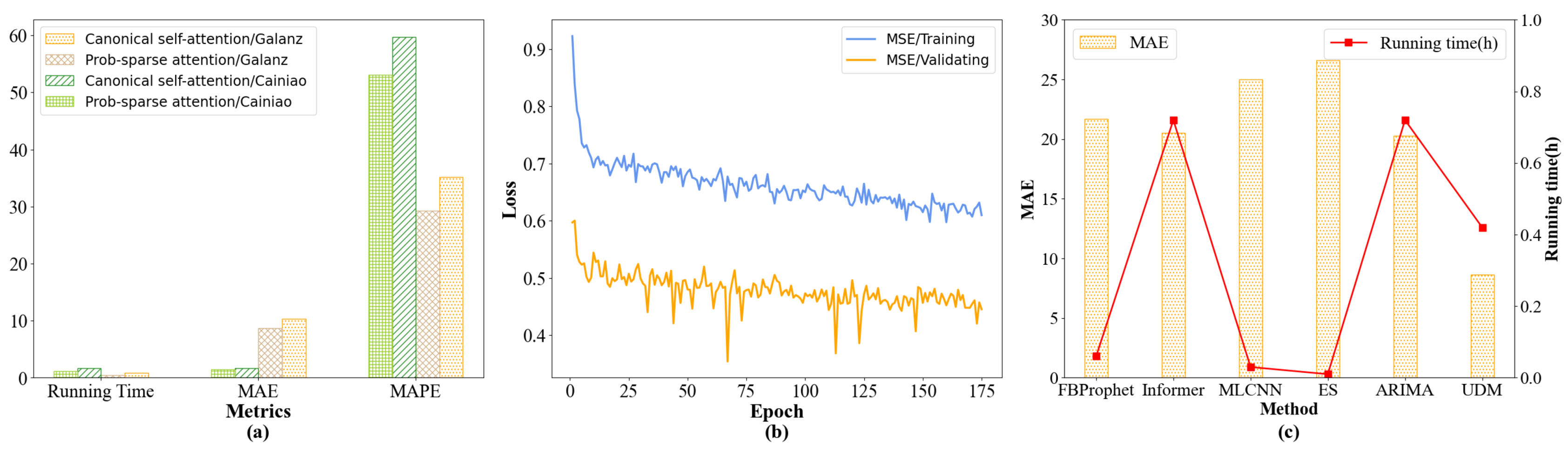
We conducted a grid search for the proposed UDM and all baselines, except ARIMA (we utilized auto-ARIMA with an automatic parameter adjustment function) to find the best hyperparameter settings. To begin with, for the task of multi-step sales sequence forecasts, we set the output length to 7, which means that the models should predict the sales sequence for 7 days. For all models, we set the maximum training iterations to 20 for the Galanz dataset and 10 for the Cainiao dataset. For UDM, we used a batch size of 16 and a learning rate of 0.0001. In the convolutional component, we set the CNN layers to 2, the dropout rate to 0.2, and the output size to 128. In the universality-extracting module, the CNN module was configured with 7 layers, the number of layers was set to 4, and the dropout rate to 0.2 for the shared GRU. Next, in the distinction-capture module, the head of the prob-sparse attention layer was 8, the sampling factor was  k = 7 , and the activation function was  g e l u . In the Pin-DTW loss function, we set the weight to  α = 1 / 2  and the target quantile to  τ = 0.6 .
For the informer model, we set  d _ m o d e l = 512 n _ h e a d s = 8 n u m _ w o r k e r s = 2 e _ l a y e r s = 2 d _ l a y e r s = 2 b a t c h _ s i z e = 16 l e a r n i n g _ r a t e = 0.0001 , and  d r o p _ o u t = 0.05 . We used MSE as the loss function and chose a prob-sparse attention mechanism in the encoder. For MLCNN, we used the continuous mode based on the data type. We applied a collaborative span of three and a collaborative stride of one. We set  l e a r n i n g _ r a t e = 0.0001 n _ C N N = 7 d r o p _ o u t = 0.2 h i d C N N = 10 h i d R N N = 25 h i g h w a y _ w i n d o w = 3 , and we tuned  k e r n e l _ s i z e [ 3 , 5 ] . For both traditional time series prediction methods, ES and FBProphet, we set alpha as 0.5 and beta as 0.9.

4.5. Main Results

We will now compare the performances of UDM and other baselines on Galanz (GW1~GW11) and Cainiao datasets (CW1~CW5), as shown in Table 3, Table 4 and Table 5. The best results are highlighted in bold, and the second-best results are underlined for each metric. Compared with traditional time series-predicting methods and advanced deep learning models, our proposed model (UDM) outperforms the other models on both Galanz and Cainiao datasets. Compared with the best baseline, the improvements are 57.27%, 50.68%, and 35.26% on the Galanz dataset and 16.58%, 6.07%, and 5.27% on the Cainiao dataset in terms of MAE, MAPE, and RMSE. For 11 Galanz warehouses datasets, UDM achieved the five best results and the five second-best results on MAE, as well as the eight best results on both MAPE and RMSE. In the Cainiao dataset, UDM demonstrated the best results in terms of MAE, MAPE, and RMSE. Among the five baselines, the informer model achieved the second-best results on the Galanz datasets. However, its prediction ability was not stable, as shown by the large MAE, MAPE, and RMSE results on several datasets, such as GW1 and GW8. Although the informer model is a very competitive baseline model, from the overall effect evaluation, UDM is significantly better than the informer model. The average improvements compared to the informer model are 20.09%, 35.26%, and 78.58% on 11 Galanz warehouses and 27.95%, 12.57%, and 31.32% on 5 Cainiao warehouses in terms of MAE, RMSE, and MAPE. Compared to all the baseline models, the informer model can achieve the 7 best MAE results and 2 best MAPE and RMSE results on 11 Galanz warehouses. However, our model achieved the best results on the whole Galanz dataset (GW1-N) and the whole Cainiao dataset (CW1-CWN) in terms of MAE, RMSE, and MAPE. For 11 Galanz warehouses and GW1-N, UDM achieved the 5 best MAE results, 10 best RMSE results, and 8 best MAPE results. For 5 Cainiao warehouses and CW1-N, UDM achieves the best results in terms of MAE, RMSE, and MAPE. In inventory management, the predicted sales component of our model serves as a reference for marketing personnel when stocking the minimum inventory level. The predicted sales component is an important indicator when arranging the inventory plan for up to two weeks in the future, and the inventory plan is based on a strict calculation process. Based on actual testing in the enterprise, our method saved approximately 20% of costs compared to traditional methods and avoids the risk of out-of-stock methods, proving its effectiveness.

4.5.1. The Advantage of the Informer

The informer is a representative transformer-based model, and is a competitive baseline model in the experiment, especially in terms of its MAE performance. Although UDM is significantly superior to the informer model on the entire Galanz datasets in terms of all metrics, the informer model outperforms UDM on 6 Galanz warehouses, in terms of the MAE metric. However, the performances of the two models on MAE are very similar; our proposed UDM model achieved comparable results to the informer model on several datasets where the informer model had previously shown superior performance, with only minor deviations. The reason for this may be that, during the independent modeling of universality and distinct aspects in UDM, information loss issues may have occurred, causing a slight decrease in UDM’s performance on the MAE metric.

4.5.2. The Advantage of UDM
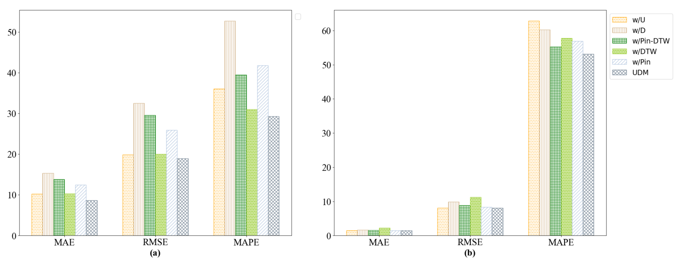
The informer model’s performance in terms of RMSE and MAPE was not as good as its performance in MAE. The MAPE of the informer model exhibited large deviations on Galanz warehouses GW1, GW6, and GW8, the MAPEs of which exceeded 300 (the MAPEs of UDM on the same warehouses were 82, 16, and 11, respectively). The reason for this is that the informer model is weaker than UDM at capturing fluctuation patterns. A large MAPE often indicates that the true number of sales is small, but the number of predicted sales is large, which means that the informer model often misjudges the sudden peak values or the fluctuation trend. UDM proposes a novel distinct mechanism, which can specifically model the unique characteristics of each time series, and learn fluctuation patterns separately. The mechanism can better solve this problem, which the informer model struggles to handle properly, and significantly improve the performance in terms of MAPE. RMSE is another metric that can evaluate the stability of the model’s performance. UDM outperformed the informer model on 8 Galanz warehouses and all Cainiao warehouses, which indicates that the performance of UDM is more stable than that of the informer model. The informer model exhibited very large variations in the testing datasets of certain Galanz warehouses. For example, the RMSE of the informer model on the dataset of Galanz warehouse GW8 was 139, while the value of UDM on the same dataset was only 31.

4.6. Ablation Study

To demonstrate the effectiveness of every UDM component, we compare UDM with five variants, as follows:
  • w/U: The universality-extracting component is removed from UDM.
  • w/D: The distinction-capture component is removed from UDM.
  • w/Pin-DTW: Pin-DTW loss is replaced by the MAE as the loss function.
  • w/DTW: DTW is removed from the Pin-DTW loss function.
  • w/Pin: Pinball loss is removed from the Pin-DTW loss function.
We kept all variant parameters the same as the completed UDM model to eliminate the influence of model complexity. Figure 3a,b present the results of the Galanz and Cainiao datasets, respectively, in detail. The important observations from these results are listed as follows:
  • Removing the distinction module causes great performance drops in terms of MAE metrics on the Galanz and Cainiao datasets; this proves that extracting the distinction module helps to achieve more accurate multi-step predictions.
  • According to Figure 3a, the significant decline in MAE appears when the Pin-DTW loss is replaced by the MAE loss function. The metrics also clearly decrease when the pinball loss is removed from the Pin-DTW loss function, which illustrates the significant contributions of the joint Pin-DTW loss function, especially the pinball loss function, to the Galanz dataset. However, Figure 3b shows that the DTW component in the Pin-DTW loss function contributes more to the Cainiao dataset.
  • Removing the universality module results in a more obvious decrease in MAE in the Galanz dataset than the Cainiao dataset, which indicates that capturing the common features of products from the same warehouse is effective in the Galanz dataset, and great differences exist between the different warehouses.
More importantly, as can be seen in Figure 3a, removing the distinction-capture component results in great drops in RMSE (41.77%) and MAPE (44.47%) in the Galanz dataset. According to Figure 3b, there are obvious decreases in performance (28.63% and 18.6%) in terms of RMSE in the Cainiao dataset when the DTW loss or the distinction-capture component is removed from UDM, and MAPE clearly goes down (15.40% and 11.83%) when the universality-extracting component or distinction-capture component is removed from UDM in the Cainiao dataset. The experimental results clearly exhibit that the distinction-capture component plays the most important role in the stability of UDM.

4.7. Further Analysis

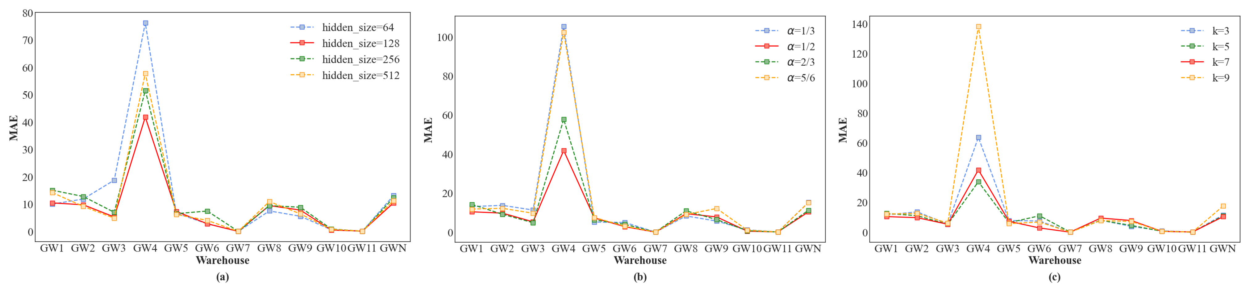
4.7.1. Parameter Sensitivity Analysis

Fine-tuning experiments on the Galanz dataset were carried out for three parameters that can obviously affect the effectiveness of the UDM. These parameters are the hidden size, the weight  α  in the Pin-DTW loss function, and the sampling factor in the distinction module. As shown in Figure 4, we attained optimal results when the hidden size was set at 128,  α  was set at  1 / 2 , and k was set at 7.

4.7.2. Comparative Analysis of Attention

We compared the canonical self-attention mechanism and the prob-sparse attention mechanism on Galanz and Cainiao datasets in terms of three metrics (running time, MAE, and MAPE), and the results can be seen in Figure 5a. From these two datasets, the prob-sparse attention mechanism performed better, with shorter running times on MAE and MAPE metrics when compared to canonical self-attention.

4.7.3. Convergence and Time Complexity Analysis
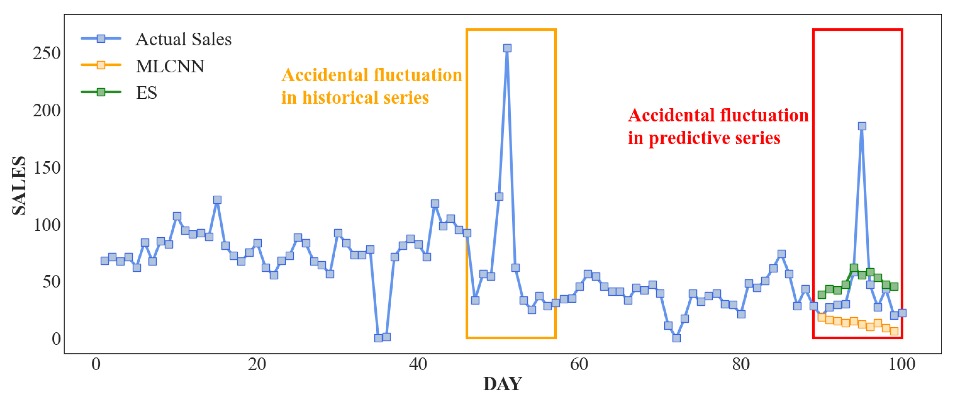
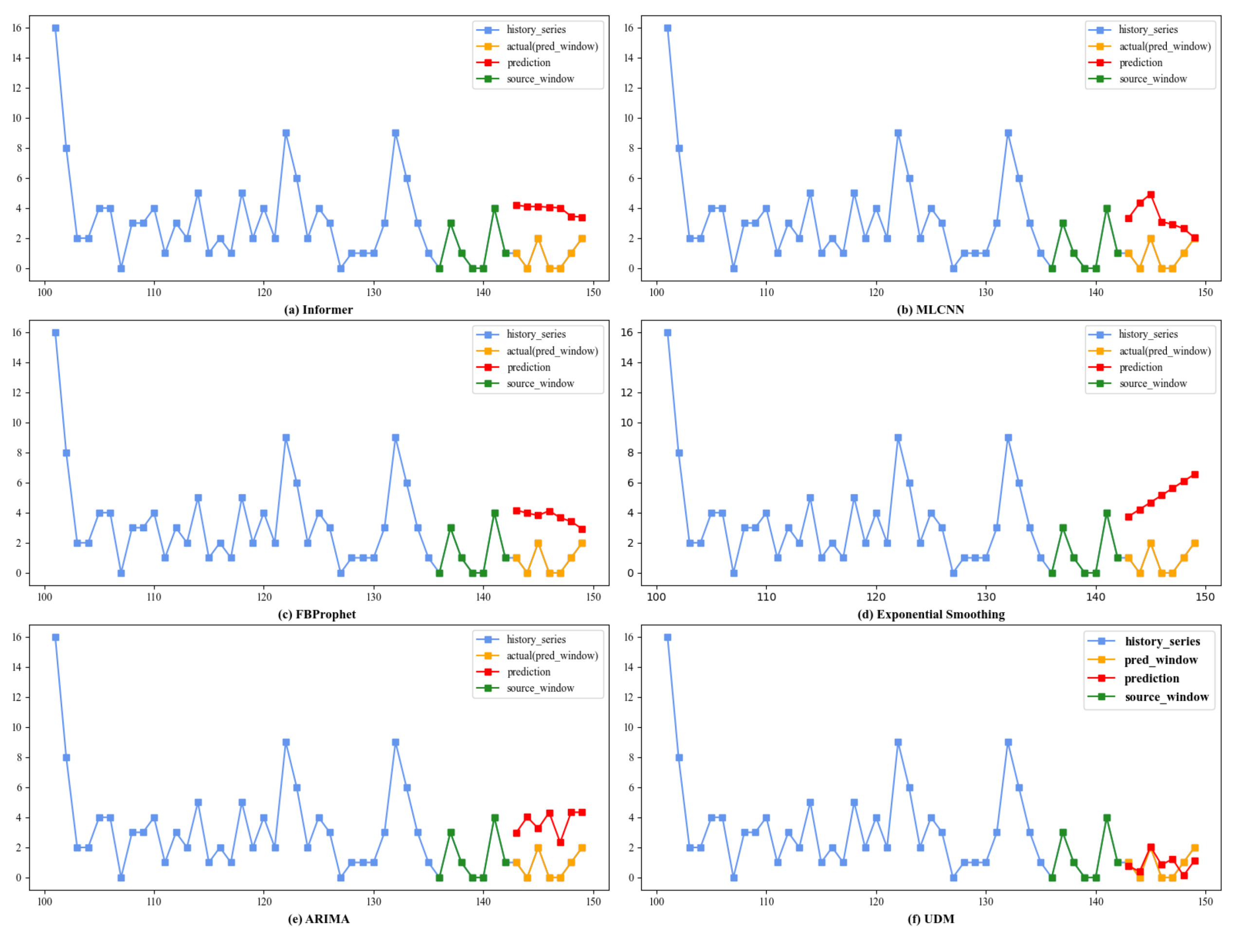
We analyzed the convergence of UDM by recording its MAE loss of training and validating on the Galanz dataset. As shown in Figure 5b, UDM can easily be trained with quick convergence. Figure 5c shows the training time and MAE comparison of FBProphet, informer, MLCNN, ES, ARIMA, and UDM on the Galanz dataset. UDM uses the attention mechanism in its distinction module, so it is reasonable that UDM takes more time for training than MLCNN, which is based on CNNs and traditional time series analysis methods (FBProphet and ES). In our study, we utilized auto-ARIMA, a model equipped with an automatic parameter tuning ability. As a result, the implementation of fitting and predicting with ARIMA requires comparatively more time. As we can see, the inference time of UDM is less than that of ARIMA and the informer model, and UDM performs better than other methods on the MAE metric.

4.8. Case Study

A case study comparing the stability in the multi-step forecast task of the proposed UDM model with five baselines can be seen in Figure 6. In this figure, the blue and green parts are used as input sequences for the prediction of item D63, where blue is a historical series and green is the source window. The yellow and red parts are found in the prediction window, in which yellow is the ground truth and red is the model prediction. In this case, the improvements in UDM for predicting the future seven-step sales are 78%, 76%, and 78%, respectively, when compared to the informer model, in terms of MAE, RMSE, and MAPE. The MAPE improvements are 74%, 73%, and 74%, respectively, compared to MLCNN. The absolute improvements in CORR are 22% and 20% compared to the informer model and MLCNN. Compared to the best performances from FBProphet, ES, and ARIMA, the improvements are 76%, 75%, and 78%, respectively, in terms of MAE, RMSE, and MAPE. Some valuable observations are as follows: (1) In our multi-step forecast tasks, the informer model provides a flat prediction and cannot simulate the real fluctuations, as shown in Figure 6a. Moreover, there is a large deviation between the predicted average and the real average. (2) The MLCNN and ARIMA models can capture fluctuations but often generate delayed predictions, resulting in an opposite change trend between actual and predicted sequences, as illustrated in Figure 6b,e. (3) The results of FBProphet are similar to those of the informer model; however, FBProphet presents a few waves that are contrary to the ground truth, which can be seen in Figure 6c. (4) The results of the exponential smoothing (ES) model are shown in Figure 6d; the errors between predictions and actual values gradually become more obvious with increasing time steps. (5) Figure 6f shows the results of the proposed UDM model, which demonstrates that not only can UDM make more accurate predictions but it can also more closely simulate the variation trend of the sales sequence compared to the baseline. Moreover, the UDM predictive accuracy remains stable in multi-step predictions. In other words, UDM achieves accurate predictions for each step, and the prediction error does not gradually increase over time steps, as seen in the ES results. The stability of our model is mainly attributed to the universality component in UDM. By extracting instinct features and common correlation patterns from multivariate time series with similar contexts, our model ensures that the multi-step predicted values remain within a reasonable range, thereby preventing error accumulation.

5. Conclusions

In our paper, we propose a novel universality–distinction mechanism framework for the multiple-step sales prediction task. Firstly, the universality-extracting module generates construals for different predictive steps, which are integrated into the complete time window information. At the same time, this module can model the relationships among different future steps and learn their universality. An efficient self-attention mechanism was then employed to distinguish the information of multiple predictive steps, which could effectively capture future fluctuations. Finally, we developed a joint Pin-DTW loss function that addresses the optimizations of two aspects of the second challenge: (1) how to make better use of the extracted common and distinct representations from UDM to make more accurate future multi-step predictions; (2) how to ensure that predicted sales are bigger than the true sales as much as possible, on the premise of minimizing prediction deviations. Both the deformation error and time delay error are seen for the first aspect, which could be solved by a sequence-based DTW loss. For the second aspect, the main aim is to avoid the risk of shortages in inventory optimization, and a pinball loss is proposed to solve this problem. The combination of pinball and DTW, named Pin-DTW loss, can reduce the risk of inventory shortage while further improving prediction accuracy and stability. The experiments conducted on the Galanz and Cainiao datasets in the Section 4 prove that our proposed UDM model ensures accurate and stable sales prediction capabilities while effectively reducing costs for enterprises.
However, some directions are worth exploring in the future. First, the outliers in the sales sequence can greatly affect the accuracy of the forecast; therefore, improving the model’s handling of outliers or abnormal values is an important direction for future research. Second, we hope to further improve the forecasting efficiency and bring real value to the enterprise supply chain.

Author Contributions

Conceptualization, D.L. and X.L.; data curation, F.G. and Z.P.; formal analysis, X.L. and F.G.; funding acquisition, D.L.; investigation, X.L., F.G. and Z.P.; methodology, D.L. and X.L.; project administration, D.L. and D.C.; resources, D.L. and D.C.; software, D.L. and X.L.; supervision, D.L. and D.C.; validation, F.G. and Z.P.; writing—original draft, X.L.; writing—review and editing, D.L. and A.M. All authors have read and agreed to the published version of the manuscript.

Funding

This research was supported by the National Natural Science Foundation of China (NSFC) under grant no. 72074231 and the Soft Science Foundation of Guangdong Province in China under grant no. 2019A101002020.

Data Availability Statement

To verify the effectiveness of the proposed model, we utilized two datasets - the Galanz dataset and the Cainiao dataset. We would release the de-identified version of the Galanz dataset at https://github.com/lx237/2023UDM once we have obtained approval from the company. The Cainiao dataset is an official dataset provided by Aliyun for a specifically designed public algorithm competition: https://tianchi.aliyun.com/competition/entrance/231530/introduction.

Conflicts of Interest

The authors declare no conflict of interest.

References

  1. Cheng, J.; Huang, K.; Zheng, Z. Towards Better Forecasting by Fusing Near and Distant Future Visions. Natl. Conf. Artif. Intell. 2020, 34, 3593–3600. [Google Scholar] [CrossRef]
  2. Harrison, P.J. Exponential Smoothing and Short-Term Sales Forecasting. Manag. Sci. 1967, 13, 821–842. [Google Scholar] [CrossRef]
  3. Slawek, S. A hybrid method of exponential smoothing and recurrent neural networks for time series forecasting. Int. J. Forecast. 2020, 36, 75–85. [Google Scholar]
  4. David, S.; Valentin, F.; Jan, G.; Tim, J. DeepAR: Probabilistic Forecasting with Autoregressive Recurrent Networks. Int. J. Forecast. 2020, 36, 1181–1191. [Google Scholar]
  5. Yudianto, M.R.A.; Agustin, T.; James, R.M.; Rahma, F.I.; Rahim, A.; Utami, E. Rainfall Forecasting to Recommend Crops Varieties Using Moving Average and Naive Bayes Methods. Int. J. Mod. Educ. Comput. Sci. 2021, 13, 23–33. [Google Scholar] [CrossRef]
  6. Breiman, L. Random Forests. Mach. Learn. Arch. 2001, 45, 5–32. [Google Scholar] [CrossRef] [Green Version]
  7. Chen, T.; Guestrin, C. XGBoost: A Scalable Tree Boosting System. Knowl. Discov. Data Min. 2016, 785–794. [Google Scholar]
  8. Lai, G.; Chang, W.C.; Yang, Y.; Liu, H. Modeling Long- and Short-Term Temporal Patterns with Deep Neural Networks. In Proceedings of the International Acm Sigir Conference on Research and Development in Information Retrieval, Ann Arbor, MI, USA, 8–12 July 2018; pp. 95–104. [Google Scholar]
  9. Lim, B.; Arik, S.O.; Loeff, N.; Pfister, T. Temporal Fusion Transformers for interpretable multi-horizon time series forecasting. Int. J. Forecast. 2021, 37, 1748–1764. [Google Scholar] [CrossRef]
  10. Zhou, H.; Zhang, S.; Peng, J.; Zhang, S.; Li, J.; Xiong, H.; Zhang, W. Informer: Beyond Efficient Transformer for Long Sequence Time-Series Forecasting. Natl. Conf. Artif. Intell. 2021, 35, 11106–11115. [Google Scholar] [CrossRef]
  11. Qin, Y.; Song, D.; Chen, H.; Cheng, W.; Jiang, G.; Cottrell, G.W. A Dual-Stage Attention-Based Recurrent Neural Network for Time Series Prediction. arXiv 2017, arXiv:1704.02971. [Google Scholar]
  12. Farnoosh, A.; Azari, B.; Ostadabbas, S. Deep Switching Auto-Regressive Factorization:Application to Time Series Forecasting. Natl. Conf. Artif. Intell. 2021, 35, 7394–7403. [Google Scholar]
  13. Zhou, Q.; Han, R.; Li, T.; Xia, B. Joint prediction of time series data in inventory management. Knowl. Inf. Syst. 2019, 61, 905–929. [Google Scholar] [CrossRef]
  14. Hmamouche, Y.; Lakhal, L.; Casali, A. A scalable framework for large time series prediction. Knowl. Inf. Syst. 2021, 63, 1093–1116. [Google Scholar] [CrossRef]
  15. Tian, H.; Xu, Q. Time Series Prediction Method Based on E-CRBM. Electronics 2021, 10, 416. [Google Scholar] [CrossRef]
  16. Malhotra, P.; Ramakrishnan, A.; Anand, G.; Vig, L.; Agarwal, P.; Shroff, G. LSTM-based Encoder-Decoder for Multi-sensor Anomaly Detection. arXiv 2016, arXiv:1607.00148. [Google Scholar]
  17. Wu, Y.; Ni, J.; Cheng, W.; Zong, B.; Song, D.; Chen, Z.; Liu, Y.; Zhang, X.; Chen, H.; Davidson, S.B. Dynamic Gaussian Mixture based Deep Generative Model For Robust Forecasting on Sparse Multivariate Time Series. Natl. Conf. Artif. Intell. 2021, 35, 651–659. [Google Scholar] [CrossRef]
  18. Eldele, E.; Ragab, M.; Chen, Z.; Wu, M.; Kwoh, C.K.; Li, X.; Guan, C. Time-Series Representation Learning via Temporal and Contextual Contrasting. arXiv 2021, arXiv:2106.14112. [Google Scholar]
  19. Pan, Q.; Hu, W.; Chen, N. Two Birds with One Stone: Series Saliency for Accurate and Interpretable Multivariate Time Series Forecasting. In Proceedings of the Thirtieth International Joint Conference on Artificial Intelligence, Montreal, QC, Canada, 19–27 August 2021; pp. 2884–2891. [Google Scholar]
  20. Chen, T.; Yin, H.; Chen, H.; Wang, H.; Zhou, X.; Li, X. Online sales prediction via trend alignment-based multitask recurrent neural networks. Knowl. Inf. Syst. 2020, 62, 2139–2167. [Google Scholar] [CrossRef]
  21. Hirche, M.; Farris, P.; Greenacre, L.; Quan, Y.; Wei, S. Predicting Under- and Overperforming SKUs within the Distribution–Market Share Relationship. J. Retail. 2021, 97, 697–714. [Google Scholar] [CrossRef]
  22. Jiang, H.; Ruan, J.; Sun, J. Application of Machine Learning Model and Hybrid Model in Retail Sales Forecast. In Proceedings of the 2021 IEEE 6th International Conference on Big Data, Xiamen, China, 5–8 March 2021; IEEE: Toulouse, France, 2021; pp. 69–75. [Google Scholar]
  23. Zhao, X.; Keikhosrokiani, P. Sales Prediction and Product Recommendation Model Through User Behavior Analytics. Cmc-Comput. Mater. Contin. 2022, 70, 3855–3874. [Google Scholar] [CrossRef]
  24. Ntakolia, C.; Kokkotiis, C.; Moustakidis, S.; Papageorgiou, E. An explainable machine learning pipeline for backorder prediction in inventory management systems. In Proceedings of the 25th Pan-Hellenic Conference on Informatics, Volos, Greece, 26–28 November 2021; pp. 229–234. [Google Scholar]
  25. Rohitash, C.; Shaurya, G.; Rishabh, G. Evaluation of Deep Learning Models for Multi-Step Ahead Time Series Prediction. IEEE Access 2021, 9, 83105–83123. [Google Scholar]
  26. Matteo, S.; Fabio, D. Robustness of LSTM neural networks for multi-step forecasting of chaotic time series. Chaos Solitons Fractals 2020, 139, 110045. [Google Scholar]
  27. Ou-Yang, C.; Chou, S.C.; Juan, Y.C. Improving the Forecasting Performance of Taiwan Car Sales Movement Direction Using Online Sentiment Data and CNN-LSTM Model. Appl. Sci. 2022, 12, 1550. [Google Scholar] [CrossRef]
  28. Paterakis, N.G.; Mocanu, E.; Gibescu, M.; Stappers, B.; van Alst, W. Deep learning versus traditional machine learning methods for aggregated energy demand prediction. In Proceedings of the IEEE Pes Innovative Smart Grid Technologies Conference, Turin, Italy, 26–29 September 2017; IEEE: Toulouse, France, 2017; pp. 1–6. [Google Scholar]
  29. Loureiro, A.L.D.; Miguéis, V.L.; da Silva, L.F.M. Exploring the use of deep neural networks for sales forecasting in fashion retail. Decis. Support Syst. 2018, 114, 81–93. [Google Scholar] [CrossRef]
  30. Qi, Y.; Li, C.; Deng, H.; Cai, M.; Qi, Y.; Deng, Y. A Deep Neural Framework for Sales Forecasting in E-Commerce. In Proceedings of the Conference on Information and Knowledge Management, Beijing, China, 3–7 November 2019; pp. 299–308. [Google Scholar]
  31. Ma, S.; Fildes, R. Retail sales forecasting with meta-learning. Eur. J. Oper. Res. 2021, 288, 111–128. [Google Scholar] [CrossRef]
  32. Yaşar, B. Comparison of Forecasting Performance of ARIMA LSTM and HYBRID Models for The Sales Volume Budget of a Manufacturing Enterprise. Istanb. Bus. Res. 2021, 50, 15–46. [Google Scholar]
  33. Chen, I.F.; Lu, C.J. Demand Forecasting for Multichannel Fashion Retailers by Integrating Clustering and Machine Learning Algorithms. Processes 2021, 9, 1578. [Google Scholar] [CrossRef]
  34. Azadi, Z.; Eksioglu, S.; Eksioglu, B.; Palak, G. Stochastic optimization models for joint pricing and inventory replenishment of perishable products. Comput. Ind. Eng. 2019, 127, 625–642. [Google Scholar] [CrossRef]
  35. Perez, H.D.; Hubbs, C.D.; Li, C.; Grossmann, I.E. Algorithmic approaches to inventory management optimization. Processes 2021, 9, 102. [Google Scholar] [CrossRef]
  36. Junyoung, C.; Caglar, G.; KyungHyun, C.; Yoshua, B. Empirical Evaluation of Gated Recurrent Neural Networks on Sequence Modeling. arXiv 2014, arXiv:1412.3555. [Google Scholar]
  37. Vaswani, A.; Shazeer, N.; Parmar, N.; Uszkoreit, J.; Jones, L.; Gomez, A.N.; Kaiser, L.; Polosukhin, I. Attention is All You Need. In Proceedings of the 31st International Conference on Neural Information Processing Systems, Long Beach, CA, USA, 4–9 December 2017; pp. 6000–6010. [Google Scholar]
  38. Shiyang, L.; Xiaoyong, J.; Yao, X.; Xiyou, Z.; Wenhu, C.; Yu-Xiang, W.; Xifeng, Y. Enhancing the Locality and Breaking the Memory Bottleneck of Transformer on Time Series Forecasting. Adv. Neural Inf. Process. Syst. 2019, 471, 5243–5253. [Google Scholar]
  39. Nikita, K.; Lukasz, K.; Anselm, L. Reformer: The Efficient Transformer. arXiv 2020, arXiv:2001.04451. [Google Scholar]
  40. Fenglin, L.; Xuancheng, R.; Guangxiang, Z.; Chenyu, Y.; Xuewei, M.; Xian, W.; Xu, S. Rethinking and Improving Natural Language Generation with Layer-Wise Multi-View Decoding. arXiv 2020, arXiv:2005.08081. [Google Scholar]
  41. Tanveer, M.; Gupta, T.; Shah, M. Pinball Loss Twin Support Vector Clustering. Acm Trans. Multimed. Comput. Commun. Appl. 2021, 17, 1–23. [Google Scholar] [CrossRef]
  42. Guen, V.L.; Thome, N. Shape and Time Distortion Loss for Training Deep Time Series Forecasting Models. Neural Inf. Process. Syst. 2019, 377, 4189–4201. [Google Scholar]
  43. Daifeng, L.; Kaixin, L.; Xuting, L.; Jianbin, L.; Ruo, D.; Dingquan, C.; Andrew, M. Improved sales time series predictions using deep neural networks with spatiotemporal dynamic pattern acquisition mechanism. Inf. Process. Manag. 2022, 59, 102987. [Google Scholar]
  44. Chikkakrishna, N.K.; Hardik, C.; Deepika, K.; Sparsha, N. Short-Term Traffic Prediction Using Sarima and FbPROPHET. In Proceedings of the IEEE India Conference, Rajkot, India, 13–15 December 2019; IEEE: Toulouse, France, 2019; pp. 1–4. [Google Scholar]
  45. Gilbert, K. An ARIMA supply chain model. Manag. Sci. 2005, 51, 305–310. [Google Scholar] [CrossRef]
Figure 1. Sales sequence analysis: the blue line represents the sequence of real sales, the green line represents the prediction of the ES model, and the orange line represents MLCNN.
Systems 11 00311 g001
Figure 2. The framework of the universality–distinction mechanism.
Systems 11 00311 g002
Figure 3. Ablation study: (a) Analysis of the Galanz dataset. (b) Analysis of the Cainiao dataset.
Systems 11 00311 g003
Figure 4. Results of the parameter sensitivity tests on the Galanz dataset. (a) Hidden size. (b) Weight of the loss function. (c) Sampling factor in the distinction module.
Systems 11 00311 g004
Figure 5. (a) Contrast between canonical self-attention and prob-sparse attention mechanisms. (b) Convergence analysis. (c) Training time analysis.
Systems 11 00311 g005
Figure 6. Case study: (a) informer, (b) MLCNN, (c) FBProphet, (d) exponential smoothing, (e) ARIMA (f) UDM.
Systems 11 00311 g006
Table 1. Variable and explain.
VariableExplain
  X n × t × b The input time series
  E h × t × b The matrix of the encoded input time series
  U t , U t + 1 , . . . , U t + k 1 The construals derived from CNNs
  O h × t × b The common correlation patterns
  Z h × t × b The distinct fluctuation signals
  f E E , f E O , f E Z Three encoder functions with self-attention for  E h × t × b O h × t × b  and  Z h × t × b
  Q S M A measurement function used to select important  q ( t )  from matrix Q for the efficient attention calculation
  f D E , f D O , f D Z Decoder functions with cross-attention
  W s g Shared weights of the GRU(Gate Recurrent Unit)  component
  W z , W r The parameters of the update gate and reset gate in the future-state GRU
  Y ^ b × k The k-step predictions for one batch
  L P i n D T W A joint  L P i n  and  L D T W  loss function
  L P i n A loss function used to prevent higher out-of-stock costs
  L D T W A loss function used to align two sequences neatly, reducing the influence of delays and fluctuations
Table 2. Information of datasets used in this paper.
DatasetGalanzCainiao
Warehouses115
Product category quantity3827
Instances583200
Sample rate1 day1 day
FeaturesProduct typeProduct type
Historical salesHistorical sales
Amount of shop discountUser visits records
Perform discount amountVisits to cart
Discount rateCollections user visits
Table 3. Evaluation of all baselines on 6 Galanz warehouse datasets (GW1-GW6). The best results are highlighted in bold, and the second-best results are underlined for each metric.
MethodMetricsGW1GW2GW3GW4GW5GW6
FBProphetMAE15.284730.304431.875534.464416.216316.7275
MAPE57.989157.167455.896862.376655.810859.6338
RMSE52.4318276.4578277.0762303.119561.225563.1584
CORR0.23730.16360.16130.21530.22480.2172
InformerMAE17.62409.15484.145029.54295.194015.0258
MAPE394.910922.500019.117680.000011.9055457.2982
RMSE35.019338.154013.021141.310722.603717.4231
CORR0.30870.00000.00000.00000.05660.2400
MLCNNMAE18.382433.605336.763837.618420.112920.7452
MAPE371.8239313.5209312.2668290.0065354.7266294.2883
RMSE60.9568281.9341286.2610308.542472.101877.0757
CORR0.21630.15970.16810.18080.20840.1929
ESMAE21.221434.133237.097140.349422.149723.0650
MAPE267.1900239.7035254.3169271.8555258.0128271.5501
RMSE63.8428292.0610294.4738320.946872.008575.0383
CORR0.19860.15890.15450.19850.19340.1985
ARIMAMAE14.229528.468030.079832.671815.304115.8134
MAPE75.127567.610966.179776.700072.441875.8649
RMSE52.2138282.8495283.7393309.138365.157366.4925
CORR0.11810.09610.09840.11540.11570.1146
UDMMAE10.41989.74075.287141.79667.30152.8003
MAPE82.768316.162616.443852.956310.294516.9803
RMSE34.268337.624712.414751.328421.78237.4525
CORR0.33730.05770.24350.54200.07030.0059
Table 4. Evaluation of all baselines over 5 Galanz warehouse datasets (GW7-GW11) and the whole Galanz dataset (GW1-N). The best results are highlighted in bold, and the second-best results are underlined for each metric.
MethodMetricsGW7GW8GW9GW10GW11GW1-N
FBProphetMAE9.085417.963428.040327.275211.248321.6805
MAPE70.781559.720758.481251.857163.392059.3717
RMSE25.179174.1755265.7824266.172440.2530155.0029
CORR0.23470.21530.16050.17160.22650.2025
InformerMAE0.0089135.43543.81775.60800.047020.5094
MAPE4.2647399.499725.750187.02971.2546136.6846
RMSE0.0945139.50188.41055.96400.181729.2440
CORR0.00000.12500.19750.09860.00970.0942
MLCNNMAE10.599321.953531.466130.628713.370025.0223
MAPE395.6474296.0490348.4923282.7980377.6082330.6571
RMSE26.179084.4675273.0667269.112343.8731162.1428
CORR0.22120.20810.15610.16350.22490.1909
ESMAE12.460424.159031.985131.654514.221026.5905
MAPE201.3380271.0901241.4655210.1611189.3783243.2783
RMSE31.493284.5216282.4325282.815943.0267167.5147
CORR0.20280.19680.16010.16160.19760.1837
ARIMAMAE7.621916.848026.403025.68379.736420.2600
MAPE74.384475.885668.507962.280370.623671.4188
RMSE23.087877.0473270.6166271.340638.8939158.2343
CORR0.13030.11800.09380.09880.12000.1108
UDMMAE0.00899.45817.79640.51140.11568.6579
MAPE2.315611.519995.49897.052810.094429.2807
RMSE0.094331.72779.68841.68390.185518.9319
CORR0.00000.10280.21980.08460.00890.1521
Table 5. Evaluation of all baselines over 5 Cainiao warehouse datasets (CW1-CW5) and the whole Cainiao dataset (CW1-N). The best results are highlighted in bold, and the second-best results are underlined for each metric.
MethodMetricsCW1CW2CW3CW4CW5CW1-N
FBProphetMAE1.59121.33461.85842.32921.79561.7818
MAPE62.164350.646967.729966.144561.528761.6429
RMSE7.54016.53277.942412.15928.30028.4949
CORR0.25320.22640.24220.24620.24800.2432
InformerMAE1.81331.58072.13392.77992.00712.0630
MAPE87.934078.379461.295066.249993.046377.3809
RMSE8.27447.20518.726813.89078.77839.3751
CORR0.24760.23690.26280.26010.24050.2496
MLCNNMAE1.71421.47522.16402.64871.82361.9651
MAPE63.325060.552494.395363.020888.935874.0459
RMSE7.83436.93329.461013.47778.87799.3168
CORR0.23530.20210.25810.23380.21900.2296
ESMAE2.04101.90122.63173.23892.32192.4269
MAPE70.347265.990386.573286.491781.685678.2176
RMSE8.31947.34409.494713.57779.51969.6511
CORR0.24490.20590.26860.23940.20800.2333
ARIMAMAE1.66121.43611.84972.53631.68701.8340
MAPE59.670649.345959.644063.641650.576156.5757
RMSE7.87527.02307.970612.69398.43148.7988
CORR0.14620.13920.14830.15270.14830.1460
UDMMAE1.36421.14981.56882.02361.32511.4863
MAPE55.686647.118755.723658.422948.757353.1418
RMSE7.28616.25597.342111.59217.75958.0472
CORR0.26800.19850.26970.20650.19670.2279
Disclaimer/Publisher’s Note: The statements, opinions and data contained in all publications are solely those of the individual author(s) and contributor(s) and not of MDPI and/or the editor(s). MDPI and/or the editor(s) disclaim responsibility for any injury to people or property resulting from any ideas, methods, instructions or products referred to in the content.

