Spatiotemporal Hybrid Air Pollution Early Warning System of Urban Agglomeration Based on Adaptive Feature Extraction and Hesitant Fuzzy Cognitive Maps

Abstract

Long-term exposure to air pollution will pose a serious threat to human health. Accurate prediction can help people reduce exposure risks and promote environmental pollution control. However, most previous studies have ignored the spatial spillover of air pollution, i.e., that the current region’s air quality is also correlated with that of geographically adjacent areas. Therefore, this paper proposes an innovative spatiotemporal hybrid early warning system based on adaptive feature extraction and improved fuzzy cognition maps. Firstly, a spatial spillover analysis model based on the Moran index and local gravitational clustering was proposed to capture the diffusion and concentration characteristics of air pollution between regions. Then, an adaptive feature extraction model based on an optimized Hampel filter was put forward to process and correct the outliers in the original series. Finally, a hesitant fuzzy information optimized fuzzy cognitive maps model was proposed to forecast the air quality of urban agglomeration. The experimental results show that the air quality forecasting accuracy of urban agglomerations can be significantly improved when the geographical conditions and other interactions among cities are comprehensively considered, and the proposed model outperformed other benchmarks and can be used as a powerful analytical tool during urban agglomeration air quality management.

1. Introduction

With the advancement of science and technology, the continuous improvement of urban spatial structure has promoted the rapid growth of the economy. But at the same time, rapid urbanization has also caused serious air quality problems [1,2]. In addition, studies have also shown that people’s long-term exposure to particulate pollutants and other air pollutants mainly includes SO₂, NO₂, O₃, and CO [3], which will cause harm to the human respiratory system, nervous system, cardiovascular system, and reproductive system [4,5,6,7]. Therefore, it is necessary to establish an air quality forecasting system to grasp the development trend of air quality and air pollution, provide technical support for regional air pollution prevention and control, and provide early warning information for daily travel or production activities.

The individual methods commonly used to forecast air quality are summarized into three types: data simulation method, mathematical statistics method, and machine learning method. The data simulation method uses professional knowledge such as atmospheric physical diffusion formulas and chemical reaction equations to simulate and forecast the formation and diffusion of pollutants [8]. This method is simple to calculate, but it needs to follow strict theoretical assumptions. Because the complexity that occurs in the atmosphere cannot be considered, forecasting accuracy is low [9]. Compared with simulation-based methods, statistical methods based on probability theory show better forecasting results. The most common are classical time series models, such as the auto-regressive (AR) models, moving average (MA) models, and auto-regressive moving average (ARMA) models [10]. However, statistical methods cannot perform nonlinear fitting during the formation and diffusion of pollutants, which leads to deviations. To address the nonlinear relationship between input and output outcomes, scholars were beginning to leverage machine learning. Support vector machine (SVM) [11,12], random foresting (RF) [13,14], and artificial neural network (ANN) [15] are widely applied in air quality forecasting. Saeid et al. used artificial neural networks to forecast PM₁₀ concentration and applied it to health risk assessment, and the correlation coefficient reached 0.87 [16]. In addition, as the historical data collected by monitoring sites increases, deep learning methods for big data show superior predictive performance. Given that the recurrent neural network (RNN) can take into account the time-dependent effects of air quality [17], it can be applied to forecast air quality by processing series well. However, in highly complex and large-scale monitoring site networks, it is difficult to capture spatiotemporal correlations between sites.

Fuzzy cognitive maps (FCM) were developed in combination with the above advantages. FCM not only has the ability to handle fuzzy logic uncertainty problems but also has the machine learning algorithms used by neural networks. The model has a good predictive effect while explaining causality [18]. For example, Liu et al. established an EMD-HFCM model combining recurrent neural networks and fuzzy logic, which greatly improved the performance of processing large-scale and non-stationary time series [19]. Yang et al. established the Wavelet-FCM model, which decomposed the original nonstationary time series into multiple time series through the wavelet transform, which improved the forecasting performance and could be applied to a variety of forecasting tasks [20]. Therefore, an in-depth study of FCM can effectively improve the performance of the model, which has the potential and advantages for dealing with dynamic, noisy air quality [21].

However, the forecasting effect of individual models is limited. So, people started building hybrid models. The multi-scale decomposition step is introduced in the forecasting system to decompose the complex system into multiple subsystems that are easy to analyze, such as decomposition and recombination methods [22], data reconstruction [23], feature extraction [24], optimization algorithms [25], etc. For example, Wang et al. applied data preprocessing based on different strategies to improve the performance of wind speed prediction systems [26]. Yang et al. added the variational mode decomposition technique based on adaptive parameters to the machine learning model, and the average absolute error of the last four data sets reached 0.5121 [27]. Hybrid models can reduce the difficulty of modeling complex systems and improve the forecasting performance of the model. Therefore, it makes sense to construct a hybrid model based on FCM.

Based on the combing and summarizing of the literature, the research motivation of this paper can be summarized as follows:

(1)

Although the hybrid model can serve the purpose of the problem well by combining specific methods, there are still some disadvantages. Most of the current hybrid models only focus on extracting data features through the decomposition of time series, which greatly improves the fitting effect of data but ignores the potential risk of information leakage in the decomposition process [28]. Therefore, the data preprocessing method needs to be further improved.

(2)

In the past, the study of air pollution was based on the division of administrative regions, and the effects of meteorology and time were analyzed separately. However, air pollution is a cross-regional environmental pollution problem, and the spatial spillover effect between urban agglomerations cannot be ignored [29].

(3)

Traditional single models cannot achieve high accuracy requirements, while hybrid models can improve forecasting accuracy.

(4)

The study of time series data only focuses on the order of time and ignores the particularities of the air quality data itself, such as the ambiguity and uncertainty of the data.

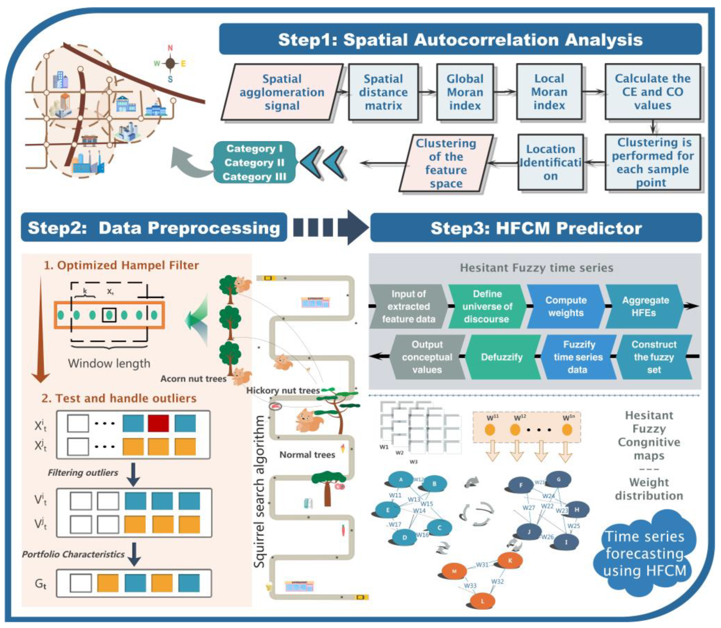
In order to solve the above problems, an innovative spatiotemporal hybrid forecasting model based on adaptive feature extraction and improved fuzzy cognitive maps is proposed. It consists of three modules: a spatial correlation analysis module, data preprocessing module, and fuzzy information forecasting module. For the spatial correlation analysis module, a spatial feature extraction model based on the Moran index and local gravitational clustering (LGC) is designed that can combine spatiotemporal features and extract key influencers from complex data to represent a variety of complex issues in a visual way. For the data preprocessing module, a novel adaptive feature extraction model optimized by the squirrel search algorithm (SSA) is proposed to process and correct the outliers of the original series. Finally, novel hesitant fuzzy cognitive maps (HFCM) are proposed for the fuzzy information forecasting module. The fuzzy logic in the original model is optimized by hesitate fuzzy information, and the forecasting at the numerical level is transformed into the forecasting of probability at the interval level.

In summary, the main contributions of this paper are:

• Spatial spillover effects are considered the main factors affecting the air quality index (AQI) of different cities. It verifies that the spatiotemporal correlation of the extracted data is necessary to improve the accuracy of air pollution forecasting.
• The Hampel filter algorithm optimized by the squirrel search algorithm is innovatively introduced into the air quality forecasting model to process and correct the data outliers to improve the forecasting accuracy of the hybrid model.
• Hesitant fuzzy cognitive maps are first proposed to forecast air pollution. It can effectively solve the gray information of air quality or fuzzy relationships and uncertainties, thus further improving the accuracy of forecasting.
• The proposed model was comprehensively evaluated with the actual AQI dataset, five model evaluation criteria, and thirteen comparative models collected from the Beijing-Tianjin-Hebei region. The empirical results show that the proposed hybrid method has superior forecasting performance compared with the comparison models and can provide a theoretical basis for air pollution forecasting and early warning.

2. Design of Spatiotemporal Hybrid Air Pollution Early Warning System

Air pollution not only has a temporal complexity but also has a spatial spillover effect. Therefore, in order to forecast air pollution scientifically and rationally, this paper proposes a spatiotemporal hybrid air pollution early warning system of urban agglomeration. Figure 1 depicts the framework of the system.

2.1. Spatial Correlation Analysis Module

In this section, the Moran I-Local gravitational clustering (ILGC) model is proposed to verify the spatial correlation and capture the diffusion and concentration characteristics of air pollution between regions.

2.1.1. Moran Index

The Moran index is applied to analyze the spatial correlation between different cities. The Moran index is divided into the global Moran index and the local Moran index [30,31]. The global Moran index is used to determine whether there is aggregation or anomaly in space, and if it is judged to be global autocorrelation, the local Moran index is further used to explore the specific manifestations of aggregation or outliers.

Global Moran index

$$I^c=\frac{{\displaystyle \sum _{i=1}^{\psi }{\displaystyle \sum _{j=1}^{\psi }{w}_{ij}(X_i^c-{\displaystyle \sum _{i=1}^{\psi }{X}_i^c/\psi })(X_j^c-{\displaystyle \sum _{j=1}^{\psi }{X}_j^c/\psi })}}}{{\displaystyle \sum _{i=1}^{\psi }{\displaystyle \sum _{j=1}^{\psi }{w}_{ij}{\displaystyle \sum _{i=1}^{\psi }{(X_i^c-{\displaystyle \sum _{i=1}^{\psi }{X}_i^c/\psi })}^2/\psi }}}}$$

(1)

Local Moran index

$$I_i^c=\frac{X_i^c-{\displaystyle \sum _{i=1}^{\psi }{X}_i^c/\psi }}{{(X_i^c-{\displaystyle \sum _{i=1}^{\psi }{X}_i^c/\psi })}^2/\psi }{\displaystyle \sum _{j\ne i}^{\psi }{w}_{ij}(X_i^c-{\displaystyle \sum _{i=1}^{\psi }{X}_i^c/\psi })}$$

(2)

where $X_i^c$ is each region $\left(i=1,2,3\dots ,\psi \right)$, c represents a different group of cities. The spatial weights between features i and j are denoted as $w_{ij}$ and the total number of features is $\psi$, so that the aggregation of all spatial weights can be found.

Most of Moran’s I belong to (−1, 1), but there are also extreme cases, that is, Moran’s value appears outside this range [32]. When Moran’s I is closer to 1, the more pronounced the positive spatial correlation and the closer the relationship between cities. When Moran’s I is closer to −1, the more pronounced the negative spatial correlation and the greater the spatial difference between cities. When Moran’s I is 0, the space is random, indicating that cities are not correlated.

2.1.2. Local Gravitational Clustering

The data are grouped using LGC based on a spatial neighborhood matrix. LGC is a clustering algorithm based on local center metrics. It describes the connectivity of the adjacent regions of each sample point through local gravitational resultant force and centrality. By comparing clustering algorithms such as k-means clustering [33] and fuzzy c-means clustering [34], LGC has the advantage of being able to train singular values to obtain possible impact information [35].

Step 1: The local resultant force is calculated for each sample point.

The local resultant force (LRF) is the sum of the forces acting at point $X_i$ with mass $m_i$, denoted as $F\left(X_i\right)$.

$$F(X_i)=\frac{1}{m_i}{\displaystyle \sum _{j=1}^k{\widehat{D}}_{ij}}$$

(3)

where the reciprocal of all distance points acting on the k nearest neighbors of the data point $X_i$ is obtained by summing up $m_i$.

$$m_i=\frac{1}{{\displaystyle \sum _{j=1}^k{D}_{ij}}}$$

(4)

$D_{ij}$ is a unit vector connecting two mass directions and k is the number of nearest neighbors around $X_i$. The closer to the center, the greater the mass of the sample points and the less susceptible they are to other forces.

Step 2: Calculate the centrality (CE) and coordination (CO) values.

The relationship between LRF is measured by two metrics: centrality and coordination. Where the centrality of data point $X_i$ is calculated as follows:

$${CE}_i=\frac{{\displaystyle \sum _{j=1}^m\cos ({\overrightarrow{F}}_j,\overrightarrow{D_{ij}})}}{m}$$

(5)

where $\overrightarrow{D_{ij}}$ is the displacement vector from $X_i$’s neighbor to $X_i$, $\cos (\theta )$ belongs to (−1, 1), and when $C{E}_i$ is greater than zero, it is pointed out that most of the neighbors point to it, indicating that it has better centrality.

The CO of data point $X_i$ is calculated as follows:

$${CO}_i={\displaystyle \sum _{j=1}^m(\overrightarrow{F_i}\cdot \overrightarrow{F_j})}$$

(6)

Among them, $\overrightarrow{F_i}$ and $\overrightarrow{F_j}$ are the local resultant forces of points $X_i$ and $X_j$, and their neighbors, and a smaller local gravitational resultant force and a larger CE value are selected as local proxy points in their own domain, and the local proxy point should preferably appear above the direction pointed by the local gravitational resultant force of the sample point.

Step 3: Clustering is performed for each sample point $X_i$.

The current local proxy point selected in the previous step connects to communicate with other local proxy points. The current local proxy point looks for the target local proxy point in the neighborhood for connection communication, and if it cannot be found, the best sample is found in the neighborhood sample, and the intermediate communication point continues to complete the work. The intermediate communication point must have a $CE$ value greater than 0 and be closer to the target proxy point than the origin. The local proxy point itself forms a small cluster, which forms a large cluster by communicating with the target proxy point.

2.2. Data Preprocessing Module

This stage introduces a new type of feature extraction model based on an improved Hampel filtering method called SHP. Since the default parameters of the adaptive Hampel filter cannot adapt to the characteristics of all data, we use the squirrel algorithm to optimize the DX (the scalar of the half-width of the filter window), T (the threshold used in the equation), and Threshold (adaptive threshold. The final minimum MAPE value is the optimization goal, and the data preprocessing algorithm for different urban agglomerations finds the best parameters and then obtains the optimal forecasting effect. The basic theoretical composition of the model is as follows.

2.2.1. Squirrel Search Algorithm

The SSA is a naturally inspired optimization paradigm that simulates the dynamic process of finding pinecones in southern flying squirrel gliding. Compared with other optimizations, SSA considers the seasonal factors of the data to be random factors, which disrupts the search space and improves the randomness of the optimization algorithm.

First, the position of the squirrel in the dimensional search space is represented using the following matrix:

$$FS=\left(\begin{array}{ccccc}F{S}_{11}& F{S}_{12}& \cdots & \cdots & F{S}_{1d}\\ F{S}_{21}& F{S}_{22}& \cdots & \cdots & F{S}_{2d}\\ ⋮& ⋮& \ddots & & ⋮\\ ⋮& ⋮& & \ddots & ⋮\\ F{S}_{n1}& F{S}_{n2}& \cdots & \cdots & F{S}_{nd}\end{array}\right)$$

(7)

where $F{S}_{nd}$ is the initial position. Next, random initialization is performed using the fol-lowing formula:

$$F{S}_i=F{S}_L+U(0,1)\times (F{S}_U-F{S}_L)$$

(8)

where $F{S}_i$ is the updated position. $U(0,1)$ denotes the randomness of the flying squirrel population contained in the range 0 to 1. $F{S}_U$ and $F{S}_L$ are the upper and lower limits, respectively.

Eventually, the squirrel colony locations are updated to the following matrix:

$$f=\left(\begin{array}{c}{f}_1\left(\begin{array}{ccccc}F{S}_{11}& F{S}_{12}& \cdots & \cdots & F{S}_{1d}\end{array}\right)\\ f_1\left(\begin{array}{ccccc}F{S}_{21}& F{S}_{22}& \cdots & \cdots & F{S}_{2d}\end{array}\right)\\ ⋮\\ ⋮\\ f_1\left(\begin{array}{ccccc}F{S}_{n1}& F{S}_{n2}& \cdots & \cdots & F{S}_{nd}\end{array}\right)\end{array}\right)$$

(9)

The difference between the advantages and disadvantages of searching for food sources will depend on the different fitness levels of each flying squirrel’s location. Therefore, based on the initial position of the squirrel, the position fitness is calculated by determining the variables, namely the best food source (hickory tree $F{S}_{ht}$), normal food source (acorn tree $F{S}_{at}$), and no food source (flying squirrel on normal tree $F{S}_{nt}$). Its position updating for three different foraging scenarios is mathematically modeled as follows.

Case 1: Best food source (hickory tree)

$$F{S}_{at}^{t+1}=\left\{\begin{array}{cc}\hspace{1em}F{S}_{at}^t+d_g{G}_c(F{S}_{ht}^t-F{S}_{at}^t)& P_{dp}\le R_1\\ \hspace{1em}Random \mathrm{location}& \mathrm{otherwise}\end{array}\right.$$

(10)

Case 2: Normal food source (acorn tree)

$$F{S}_{nt}^{t+1}=\left\{\begin{array}{cc}\hspace{1em}F{S}_{nt}^t+d_g{G}_c(F{S}_{at}^t-F{S}_{nt}^t)& P_{dp}\le R_2\\ \hspace{1em}Random \mathrm{location}& \mathrm{otherwise}\end{array}\right.$$

(11)

Case 3: No food source (flying squirrel on normal tree)

$$F{S}_{nt}^{t+1}=\left\{\begin{array}{cc}\hspace{1em}F{S}_{nt}^t+d_g{G}_c(F{S}_{nt}^t-F{S}_{nt}^t)& P_{dp}\le R_3\\ \hspace{1em}Random \mathrm{location}& \mathrm{otherwise}\end{array}\right.$$

(12)

where $d_g$ is the random glide distance, $R_1,R_2,R_3$ is a random number in the range of [0, 1], $F{S}_{nt}^{t+1}$ is the position of the squirrel reaching the hickory tree, and t is the current iteration. The sliding constant $G_c$ is used in the mathematical model to seek a balance between exploration and development. Its value has a non-negligible role in the performance of the proposed algorithm. In the current work, the value of $G_c$ is 1.9, which is derived from rigorous analysis. The predator presence probability $P_{dp}$ is 0.1 in all cases.

At the same time, in winter, due to low-temperature environmental conditions, squirrels tend to exercise on a small scale compared to other seasons and are mostly used to store pecans to maintain energy for the winter, so the influence of seasonal factors is considered. It can effectively solve the problem that the algorithm is trapped in the local optimal solution. Seasonal variables are expressed as:

$$S_c^t=\sqrt{{\displaystyle \sum _{k=1}^d{(F{S}_{at,k}^t-F{S}_{ht,k}^t)}^2}}$$

(13)

$$S_{min}=\frac{10H^{-6}}{{\left(365\right)}^T{(T_m/2.5)}^{-1}}$$

(14)

where k is the current iteration value and $S_{min}$ is a direct influence on the algorithm’s search and development capability. The larger the $S_{min}$, the stronger the exploration capability, and the smaller the $S_{min}$, the stronger the development capability.

After winter, flying squirrel foraging will be active again, considering that those squirrels that have not been able to find the best food source in winter but still survive will be able to forage again, and there is randomness, which will move in different directions.

The repositioning of the flying squirrel can be expressed by the equation as:

$$F{S}_{nt}^{new}=F{S}_L+Lévy(n)(F{S}_U-F{S}_L)$$

(15)

where $F{S}_U$ and $F{S}_L$ are the upper and lower bounds of variables, $Lévy$ is used to generate random solutions.

$$Lévy(x=0.01\times \frac{r_a\sigma }{{\left|r_b\right|}^{1/\beta }})$$

(16)

where $r_a$ and $r_b$ are random number matrices belonging to (0, 1), $\beta$ = 1.5. And $\sigma$ is defined as follows:

$$\sigma ={\left(\frac{\Gamma (1+\beta )\sin (\frac{\beta \pi }{2})}{\Gamma (\frac{1+\beta }{2})\beta 2^{(\frac{\beta -1}{2})}}\right)}^{1/\beta }$$

(17)

where $\Gamma \left(x\right)=\left(x-1\right)!$.

2.2.2. Hampel Filter

The Hampel filter is a decision filter used to detect and remove outliers [36]. Like the $3\sigma$ rule, which distinguishes between the mean and standard deviation, it determines whether the data in the data set are a singular value by the median and the median that deviates from the absolute value of the median, and then replaces the outlier with the median of the short series in the filter movement window.

$$\left|x_i-x^{\ast }\right|>tS\hspace{1em}j=1,2,\dots ,N$$

(18)

$$S=1.4286median\left\{\left|x_i-x^{\ast }\right|\right\}$$

(19)

where t is a predefined threshold for determining the absolute difference from the median, and $x^{\ast }$ denotes the median of the data sequence of length N, and S is the median absolute difference (MAD) scale estimator. The constant 1.4286 guarantees that the expected value of S is equal to the standard deviation of the normal distribution data [37].

2.3. Fuzzy Information Forecasting Module

In this section, the basic theory of hesitant fuzzy time series is first described, followed by the details of the innovative hesitant fuzzy cognitive maps. This paper innovatively proposes hesitant fuzzy cognitive maps (HFCM) and introduces the hesitant fuzzy logic relationship to modify the output results of the fuzzy cognitive maps.

2.3.1. The Basic Definition of Hesitant Fuzzy Theory

Before constructing hesitant fuzzy cognitive maps for forecasting, let us review the definitions of fuzzy set, hesitant fuzzy set, and fuzzy time series (FTS). The basic theory is as follows [38].

Definition 1.

Define $U=\left\{u_1,u_2,\cdots ,u_n\right\}$ the universe of discourse. A fuzzy set $A_{ij}$ in U can be defined by its membership function.

$$A_{ij}={\displaystyle \sum _{i=1}^n{\displaystyle \sum _{j=1}^m\frac{\mu A_{ij}(x_{ij})}{x_{ij}}}}=\frac{\mu A_{11}(x_{11})}{x_{11}}+\frac{\mu A_{12}(x_{12})}{x_{12}}+\cdots +\frac{\mu A_{nm}(x_{nm})}{x_{nm}}$$

(20)

where $A_{ij}:U\to [0,1]$ represents the membership function of the fuzzy set $A_{ij}$ and $\mu A_{ij}$ represents the member degree of µ to $A_{ij}$.

Definition 2.

$H,A_{ij},X$ over the reference set $U=\left\{u_1,u_2,\cdots ,u_n\right\}$ is represented by a mathematical expression as follows:

$$H=\left\{〈x_{ij},h_H(x_{ij})〉\left|\forall x_{ij}\in U\right.\right\}$$

(21)

where $h_H\left(x_{ij}\right)$ is the set of possible subsets in [0, 1] by membership function that computes the possible membership degrees of the elements in U to the set H. $P[0,1]$ is the set of multiple subsets of [0, 1]. For the element $u\in U$, $h_H\left(u_i\right)$ is called the hesitant fuzzy element (HFE).

Definition 3.

Let $Y\left(\xi \right) \left(\xi =0,1,2,\dots \right)$ , R (a subset of real number) be a universe of discourse. Different fuzzy sets $f_i\left(\xi \right) \left(\xi =0,1,2,\dots \right)$ are defined on $Y\left(\xi \right)$. If $F\left(\xi \right)$ is a collection of $f_i\left(\xi \right) \left(\xi =0,1,2,\dots \right)$, then it is known that $F\left(\xi \right)$ is called an FTS on $Y\left(\xi \right) \left(\xi =0,1,2,\dots \right)$.

Definition 4.

Let $F\left(\xi \right)$ be the FTS and $R\left(\xi ,\xi -1\right)$ be a first order model of $F\left(\xi \right)$. If $R\left(\xi ,\xi -1\right)=R\left(\xi -1,\xi -2\right)$ for any time  $\xi$, then $F\left(\xi \right)$ is designated as time-invariant FTS, otherwise $F\left(\xi \right)$ is named as time-variant FTS.

Definition 5.

The fuzzy logic relation (FLR) can be expressed as $F(\xi -q)\to F(\xi )$, Their relationship can be expressed by the formula:

$$F(\xi )=F(\xi -q)oR(\xi -q,\xi )$$

(22)

where “$o$” is a max-min composition operator, $R(\xi -q,\xi )$ is fuzzy relationship.

Definition 6.

The relationship between $F(\xi )$ and $F(\xi -q)$ can be denoted as $A_w\to A_v$ , where $A_w$ and $A_v$ are called the left-hand side and the right-hand side of the FLR, respectively. FLRs with the same left-hand side can be categorized into an ordered fuzzy logic group (FLG).

2.3.2. The FCM Framework

FCM consists of a set of nodes and weighted edges, which can be regarded as a weighted directed graph. The nodes represent the variables in the AQI time series, that is, each city in the urban agglomeration, and the edges represent the causal relationship between these nodes. The set of these concept nodes is represented as vector C, that is, the set of urban agglomerations. Each FCM containing N concepts can be defined by four elements, $\left(C,W,A,F\right)$, where $C=\left\{C_1,C_2,\cdots ,C_N\right\}$ is the collection of concepts that represent all detected air quality indices. These concepts define the state value of t at any moment as a vector $A_i$, that is, the AQI time series data of each city:

$$A_i=\left\{A_1,A_2,\cdots ,A_N\right\}$$

(23)

where $W^c:C\times C\to [-1,1]$ is an $N\times N$ connection matrix representing the relationship from $C_i$ to $C_j$.

The circular relationship between $A\left(\xi -1\right)$ and $A\left(\xi \right)$ on $\xi \ge 0$ is expressed as follows:

$$A_i^c\left[k+1\right]=f\left(A_i^c\left[k\right]+{\displaystyle \sum _{j=1,j\ne i}^m\left(A_i^c\left[k\right]W_{ij}\right)}\right)$$

(24)

$A_i^c\left(\xi \right)$ denotes the state value of node $A_{\mathrm{i}}^c$ at time $\xi$, $A_i^c\left(\xi +1\right)$ denotes the value of node $A_i^c$ at time $\xi +1$. The state value of the node at the (t + 1)-th iteration is determined by the weight matrix and state value of all connected nodes at the t-th iteration.

The f is the transfer function which simulates the forecasting process of the conceptual state of the c-th FCM model. It is the activation function that updates the activation state of the node at each iteration to perform a simulation of conceptual state forecasting.

$$f(x)=\frac{1}{1+e^{-\lambda x}}$$

(25)

where $\lambda \left(\lambda \ge 0\right)$ acts as a regulator that determines the appropriate shape of the function and the speed at which the curve converges to the boundary. $\lambda =1$ is commonly chosen.

2.3.3. Hesitant Fuzzy Processing Time Series

• Step 1: Define the universe of discourse and divide the interval.

The universe of discourse is defined as $U=[D{a}_{\min }-{\sigma }_1,D{a}_{\max }+{\sigma }_2]$. Among them, $D{a}_{\max }$ and $D{a}_{\min }$ are the maximum and minimum values of AQI data, respectively, ${\sigma }_1$ and ${\sigma }_2$ are the standard deviation of the training sample.

Then, the cumulative distribution function (CDF) is used to divide the equal frequency interval.

$$F(x_i^c)=\mathrm{Pr}(X\le x_i^c)for-\infty <x_i^c<\infty$$

(26)

To determine the optimal number of intervals, adaptive interval division is performed based on fuzzy c-means clustering. The cluster generated by clustering is regarded as a fuzzy set; the cluster center is the midpoint of the interval, and the size of the clustered category is the interval size.

$$u_{ij}^c=\frac{1}{{\displaystyle \sum _{center=1}^k{(\raisebox{1ex}{$d_{ij}^c$}\!\left/ \!\raisebox{-1ex}{$d_{ik}^c$}\right.)}^{\raisebox{1ex}{$2$}\!\left/ \!\raisebox{-1ex}{$fz-1$}\right.}}}$$

(27)

where $u_{ij}^c$ is the membership degree between the sample point $x_i^c$ and the cluster enter $v_j^c$, i is the sample, c is the city category, $f_z$ is the fuzzy index ($f_z>1$), $d_{ij}^c$ is the distance between the sample point $x_i^c$ and cluster center $v_j^c$. The most common method for calculating the distance is Euclidean distance.

$$v_j^c=\frac{{\displaystyle \sum _{i=1}^n{(u_{ij}^c)}^{f_z}{x}_i}}{{\displaystyle \sum _{i=1}^n{(u_{ij}^c)}^{f_z}}}$$

(28)

• Step 2: Calculate membership degree.

For the calculation of the weights $w_e^h$, $w_u^h$, this article uses the trigonometric membership function with the following formula:

$$w_e^h=\frac{d_e}{d_e+d_u}$$

(29)

$$w_u^h=\frac{d_u}{d_e+d_u}$$

(30)

where $d_e$ and $d_u$ are the equal and unequal spacing lengths calculated above, respectively.

The triangle membership function is used to calculate the membership degree on the interval divided by different methods, and the $mbge\left(i\right)$, $mbgu\left(i\right)$ is obtained. The triangle membership function formula is as follows:

$$triangle(x_i^c;a,b,c)=\left\{\begin{array}{ccc}0& & x_i^c\le a\\ \frac{x_i^c-a}{b-a}& & a\le x_i^c\le b\\ \frac{c-x_i^c}{c-b}& & b\le x_i^c\le c\\ 0& & c\le x_i^c\end{array}\right.$$

(31)

The formula for aggregating hesitant fuzzy elements and constructing fuzzy sets, where the aggregation operator is used to calculate the member rank of the elements, is defined as follows:

$$O\left\{x_1,x_2,\cdots ,x_n\right\}=1-{\displaystyle \prod _{i=1}^n{\left(1-x_i\right)}^{w_i^h}}$$

(32)

Based on Definition 3, the fuzzy set is determined according to the maximum membership principle. Because the air quality index lags one-stage correlation, the first-order fuzzy logic relationship is determined according to Definition 5. After that, the fuzzy relationship group is established based on Definition 6 by counting the frequency of fuzzy relationships in the training set.

• Step 3: Build fuzzy relationship matrix.

The weight matrix is established by the elements in the fuzzy relationship matrix with the frequency of “$A_w\to A_v$” in the training set.

$$\left(\begin{array}{cccc}{w}_{11}& w_{12}& \cdots & w_{1m}\\ w_{21}& w_{22}& \cdots & w_{2m}\\ ⋮& ⋮& \ddots & ⋮\\ w_{m1}& w_{m2}& \cdots & w_{mm}\end{array}\right)=\left[W_1^c,W_2^c,\cdots ,W_m^c\right]$$

(33)

where $w_{ij}\in [0,1],\left(i,j=1,2,\dots ,m\right)$. It is the result of weighting the frequency of each fuzzy relationship.

• Step 4: Defuzzify

Fuzzy output is obtained on the basis of hesitant fuzzy relations. Before that, the combined midpoints of the equal and unequally spaced trigonometric membership functions are calculated as follows:

$$CM=\frac{M_e{w}_e^h+M_u{w}_u^h}{e_e^h+e_u^h}$$

(34)

where $M_e$; $w_e^h$ and $M_u$; $w_u^h$ are the midpoints and weights of the membership functions in the interval of equality and inequality, respectively. Use the following formula to defuzzify them for numerical forecasting.

$$NF=\frac{{\displaystyle \sum f_{i}C{M}_i}}{{\displaystyle \sum f_i}}$$

(35)

where $f_i$ is the fuzzified output obtained by applying the max–min combination operation on fuzzy logic relationships (FLR).

The pseudo-code of the data hesitant fuzzification process of Algorithm 1 is as follows:

Algorithm 1: HFCM
Objective function: min (MAPE) =$\frac{1}{n}{\displaystyle \sum _{i=1}^n\left|\frac{{\widehat{y}}_i(x)-y_i(x)}{y_i(x)}\right|}\times 100\%$
Input: $\left(x_1^c,x_2^c,x_3^c,\dots ,x_n^c\right)$—a sequence of sample data.    $\left(h_1^c,h_2^c,h_3^c\dots h_n^c\right)$—a sequence of FCM output Output: $\left\{\begin{array}{c}MAPE(r,:)=\frac{1}{n}{\displaystyle \sum _{i=1}^n\left|\frac{{\widehat{y}}_i(x)-y_i(x)}{y_i(x)}\right|}\times 100\%\\ RMSE(r,:)=\sqrt{\frac{1}{n}{\displaystyle \sum _{i=1}^n{\left(y_i(x)-y_i(x)\right)}^2}}\\ MAE(r,:)=\frac{1}{n}{\displaystyle \sum _{i=1}^n\left|{\widehat{y}}_i(x)-y_i(x)\right|}\end{array}\right.$
Parameters: ip: number of the intervals i: i-th sample j: $\left\{\begin{array}{cc}0\hfill & adaptive division interval\\ 1\hfill & equal frequency division interval\end{array}\right.$ $Lo(N)$: the left endpoint of the adaptive division interval $Up\left(N\right)$: the right endpoint of the adaptive division interval $P_{LB}\left(N\right)$: the left endpoint of the equal frequency division interval $P_{UB}\left(N\right)$: the right endpoint of the equal frequency division interval $mbge\left(i\right)$: the membership degree of the adaptive division interval $mbgu\left(i\right)$: the membership degree of the equal frequency division interval nn: min number of the intervals mm: max number of the intervals
1:	/* Initialize the data and convert it into growth rate */
2:	/* Define the universe of discourse */
3:	FOR ip = nn: mm (number of the intervals); N = ip;
4:		/* Calculate $Lo(N);Up(N)$ by cumulative distribution function. (Equation (26)) */
5:		/* Calculate $P_{LB}\left(N\right);P_{UB}(N)$ by fuzzy c-means clustering (Equation (27)) */
6:		/* Calculate the weights of different intervals */
7:		$de=P_{UB}(N)-P_{LB}(N), du=Up\left(N\right)-Lo\left(N\right)$;
8:		$we=de/\left(de+du\right), wu=du/\left(de+du\right)$
9:		/* Calculate $mbge\left(i\right); mbgu(i)$ */
10:		Calculate: Membership grades $u(i)=1-({(1-mbge(i))}^{we})\times ({(1-mbgu(i))}^{wu})$;
11:		/* Judgment fuzzy sets */$u_{ki}=max (u_{1i},u_{2i},u_{3i}\dots .,u_{ji}),1<k<n$
12:			IF $H_{Ak}$ is fuzzy set corresponding to$u_{ki}$
13:				Assign fuzzy set $H_{Ak}$ to $x_i^c$
14:			END
15:			IF$H_{Ai}$ is fuzzy production of day n, and $H_{AK}$ is fuzzy production of day n + 1
16:				$Fuzzy logic relationship=\left\{H_{A1}-H_{A2}, \dots , H_{Ai}-H_{Aj}\right\}$
17:			END
18:		/* Determine the fuzzy logic relation group */
19:		/* Count the frequency of each logical relationship */
20:		/* Calculate the percentage rate of each occurrence logic */
21:		/* Calculate the weight matrix and normalize the weight. */
22:		Calculate:  $grade\left(i,j\right)=trimf \left(\left(h_1^c,h_2^c,h_3^c\dots h_n^c\right), \left[Lower\left(j\right) , mid\_point\left(j\right), Upper(j)\right]\right)$;
23:		/* The maximum membership principle determines the fuzzy set to which it belongs. */
24:		Calculate: $combined mid=\left(we. *mid\_point\left(j\right)+wu. *mid\_point\left(j\right)\right). /\left(we+wu\right)$;
25:		/* Defuzzification to obtain the predicted value */
26:		/* Turning growth rates into data ${\widehat{y}}_i(x)$ */
27:	END
28:	$\left[r,c\right]=find\left(MAPE==min\left(MAPE\right)\right)$
29:	Returned: r (The location of the optimal concept)

2.4. Error Evaluation Module

To evaluate the superiority of the proposed system, the error evaluation module was constructed, which contained three statistical indicators and two test models.

2.4.1. Error Test

The following three statistical indicators were employed to evaluate the effectiveness of the predictive model: mean absolute percentage error (MAPE), root mean square error (RMSE), and mean absolute error (MAE). They are defined as:

$$MAPE=\frac{1}{n}{\displaystyle \sum _{i=1}^n\left|\frac{{\widehat{y}}_i(x)-y_i(x)}{y_i(x)}\right|}\times 100\%$$

(36)

$$RMSE=\sqrt{\frac{1}{n}{\displaystyle \sum _{i=1}^n{\left(y_i(x)-y_i(x)\right)}^2}}$$

(37)

$$MAE=\frac{1}{n}{\displaystyle \sum _{i=1}^n\left|{\widehat{y}}_i(x)-y_i(x)\right|}$$

(38)

where ${\widehat{y}}_i(x)$ is the forecasting data, $y_i(x)$ is the original data, and i is the number of samples.

2.4.2. Hypothesis Testing

This section uses the Diebold–Mariano (DM) test [39] and the modified Diebold–Mariano (MDM) test [40] to evaluate hypothesis testing methods for the predictive performance of different models. Its theory is described below.

The raw data is $\left\{u_t^n\right\}$, and for the two forecasting sequences $\left\{{\epsilon }_{jt}\right\}$ and $\left\{{\epsilon }_{kt}\right\}$, their error can be calculated by the following formula:

$$e{r}_{jt}^n={\epsilon }_{jt}-u_t^n$$

(39)

$$e{r}_{kt}^n={\epsilon }_{kt}-u_t^n$$

(40)

$$\psi \left(e{r}_{jt}^n\right)={\left(e{r}_{jt}^n\right)}^2$$

(41)

$$\psi \left(e{r}_{kt}^n\right)={\left(e{r}_{kt}^n\right)}^2$$

(42)

At this point, the difference between the two error sequences $\left\{dif{f}_t\right\}$ can be defined as follow:

$$dif{f}_t=\psi \left(e_{jt}^n\right)-\psi \left(e{r}_{kt}^n\right)$$

(43)

The null and alternative hypotheses are set as follows:

$$\begin{gathered} H_0:E\left(dif{f}_t\right)=zero; \\ {H}_1:E\left(dif{f}_t\right)\ne zero; \end{gathered}$$

The DM statistic follows a standard normal distribution and can be calculated as:

$$DM=\overline{diff}/\sqrt{S^2/T-1}$$

(44)

Specifically, T is the number of advance multi-step forecasting. Where $\overline{diff}$, $S^2$ can be defined as:

$$\overline{diff}=T^{-1}{\displaystyle \sum _{t=1}^{T}dif{f}_t}$$

(45)

$$S^2={\left(T-1\right)}^{-1}{{\displaystyle \sum _{t=1}^T\left(dif{f}_t-\overline{diff}\right)}}^2$$

(46)

However, efficient T-period forecasting has forecasting errors after the $MA\left(\mathrm{T}-1\right)$ process, so MDM is proposed to solve this problem with the assumption that “no observed” lag has zero covariance. The DM statistic is compared with the cut-off value $Z_{\alpha /2}$. If $-Z_{\alpha /2}\le DM\le Z_{\alpha /2}$, accept the null hypothesis, indicating that there is no difference in the forecasting effect of the two models; If $DM>Z_{\alpha /2}$ or $DM<Z_{\alpha /2}$, the null hypothesis was rejected, indicating that the difference in forecasting performance between the two models was not caused by accidental factors.

3. Results

This section includes three parts: data description, spatial feature capture, and model comparison experiments. What is more, three sets of comparison experiments are established to verify the validity of the forecasting of the proposed spatiotemporal mixture model.

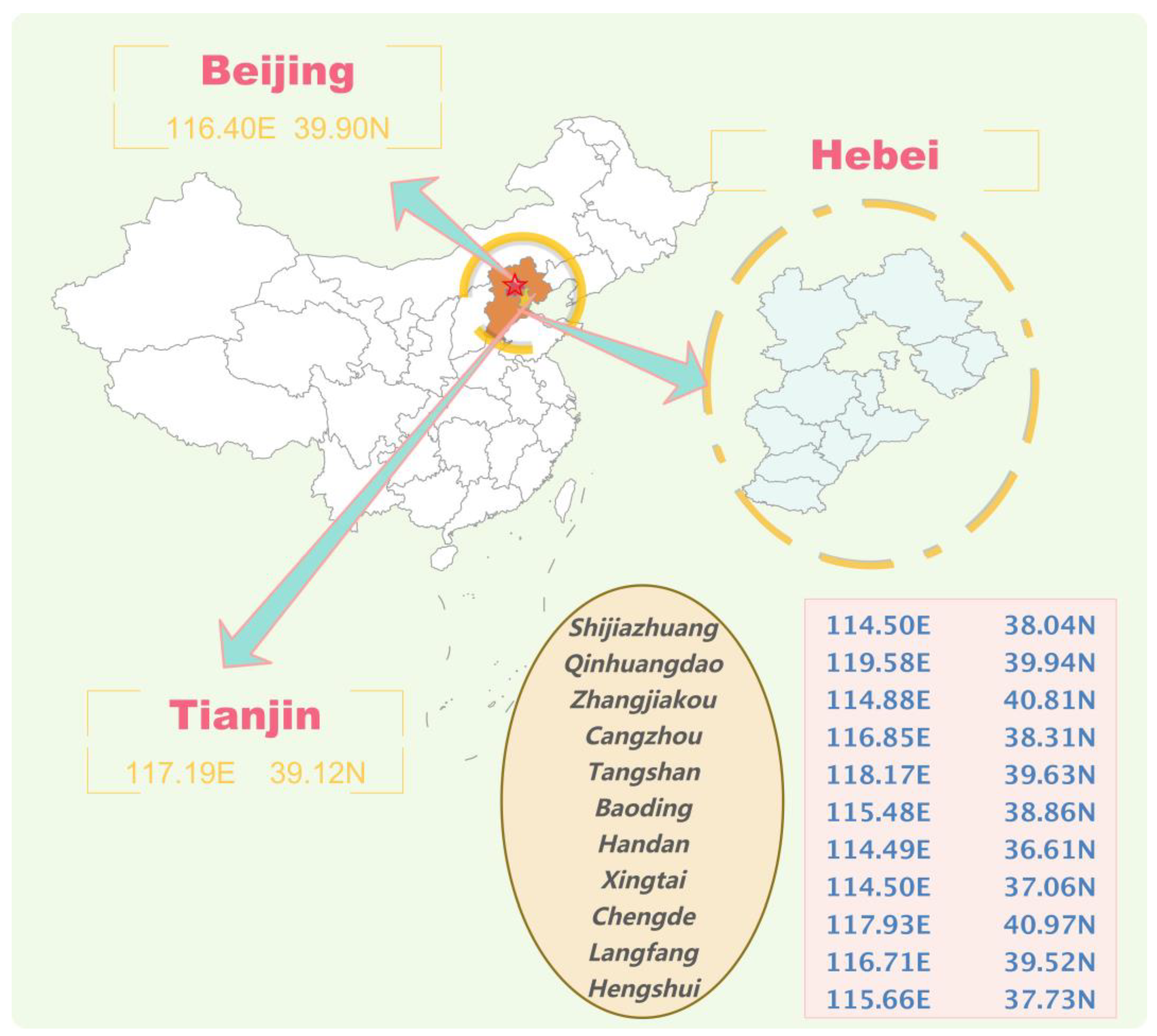
3.1. Study Area and Data Description

To verify the accuracy and effectiveness of the proposed model, the Beijing-Tianjin-Hebei region was selected as the research object. The site of the study is shown in Figure 2.

China’s major urban agglomerations with high levels of economic development are Beijing-Tianjin-Hebei, Yangtze River Delta, and Pearl River Delta. Among them, the Beijing-Tianjin-Hebei region is not only a representative area of China’s economic development but also a typical area with serious air pollution [41]. Due to the high population density in the region, the proportion of heavy industry [42], industrial transfer [43], and other factors, the air environment problem has become increasingly prominent. While the Beijing-Tianjin-Hebei region has coordinated economic development [44], air quality between different cities also has a certain mutual influence [45]. The air pollution problem of the Beijing-Tianjin-Hebei urban agglomeration has become a topic of general concern for the Chinese government, the media, and the public. So, it is typical to select the Beijing-Tianjin-Hebei region as the research object.

This study uses daily AQI data from 1 January 2017 to 31 August 2022, for 13 cities with a total of 2069 observations. Daily AQI data were collected from http://www.tianqihoubao.com (accessed on 10 September 2022). AQI is a comprehensive indicator of air quality [46], and the higher the value, the more serious the pollution. It was calculated according to the National Ambient Air Quality Standard of China (GB3095-2012) [47], including sulfur dioxide (SO₂), nitrogen dioxide (NO₂), PM_2.5, PM₁₀ (particulate matter with particle size less than or equal to 10 μm), ozone (O₃), carbon monoxide (CO), and other six pollutants [18] to comprehensively reflect the regional air quality and pollution degree. Comprehensive AQI can emphasize the possible chronic health effects of air pollution and long-term damage to the environment. Compared with the air pollution index (API) [48], the detection of pollutants is more comprehensive, the grading restriction standards are stricter, and the evaluation results are more objective. Specifically, the air pollution level is divided into seven attribute categories according to the air quality index (AQI), as shown in

Table 1. Air quality index scale.

AQI	Level	I	Descriptions	Color
0–50	I	0.155	Good	Green
51–100	II	0.207	Moderate	Yellow
101–150	III	0.176	Lightly polluted	Orange
151–200	IV	0.095	Moderately polluted	Red
201–300	V	0.066	Heavily polluted	Purple
>300	VI	0.195	Severely polluted	Maroon

.

When the air pollution index is less than 100, people can engage in normal activities. When the air quality index reaches mild pollution (100~200), patients with heart disease and respiratory diseases should reduce physical consumption and outdoor activities; when the air quality index reaches 200~300, healthy people ought to reduce outdoor ac-tivities. Additionally, the elderly and patients with heart disease and lung disease should stay indoors and reduce physical activity; when heavy pollution (air quality index above 300) is reached, healthy people should also avoid outdoor activities.

Statistical analysis of daily data is shown in

Table 2. Statistical analysis of raw data.

No.	City Name	Longitude	Latitude	Training	Testing	Max	Min	Mean	Std
1	Shijiazhuang	114.502461	38.045474	1656	413	442	19	97.85	57.78
2	Hengshui	115.665993	37.735097	1656	413	377	16	89.68	50.88
3	Baoding	115.482331	38.867657	1656	413	476	17	92.46	56.39
4	Xingtai	114.508851	37.068256	1656	413	463	17	97.28	56.61
5	Handan	114.490686	36.612273	1656	413	389	16	99.81	56.43
6	Beijing	116.405285	39.904989	1656	413	454	11	72.05	47.77
7	Cangzhou	116.857461	38.310582	1656	413	346	16	81.99	45.15
8	Langfang	116.713873	39.529244	1656	413	413	13	78.05	46.25
9	Tianjin	117.190182	39.125596	1656	413	365	14	78.29	42.51
10	Tangshan	118.175393	39.635113	1656	413	399	16	84.83	45.85
11	Chengde	117.939152	40.976204	1656	413	409	17	59.69	31.20
12	Qinhuangdao	119.586579	39.942531	1656	413	364	16	66.22	35.44
13	Zhangjiakou	114.884091	40.811901	1656	413	488	19	59.34	36.17

.

From Table 2, in the Beijing-Tianjin-Hebei region, Shijiazhuang and Chengde have the best air quality situation, with mean values of 59.69 and 59.34, respectively, and less fluctuation, with variances of 31.2 and 36.17. In comparison, Handan has the worst air quality and a larger variation, indicating that the air pollution level fluctuates more seri-ously in the process of economic and social development.

3.2. Spatial Feature Extraction Results

For each city, the annual average of daily AQI data is taken as the data for Moran’s index, and the geographical distance matrix is used to describe the static spatial correlation between cities, so as to further use the model to summarize the neighborhood characteristics of the target city for spatiotemporal forecasting.

3.2.1. Spatial Autocorrelation

Table 3. Moran index of the AQI for 2017 and 2022.

Year	I	E(I)	Sd(I)	z	p-Value *
2017	0.155	−0.083	0.092	2.599	0.005
2018	0.207	−0.083	0.092	3.164	0.001
2019	0.176	−0.083	0.09	2.873	0.002
2020	0.095	−0.083	0.09	1.983	0.024
2021	0.066	−0.083	0.09	1.661	0.048
2022	0.195	−0.083	0.091	3.064	0.001

Note: I is Moran’s index, reflecting the spatial correlation. E(I) is the mean of I, Var(I) is the standard deviation of I; Z is the standard score, reflecting the degree of dispersion of a data set; p-value rep-resents the probability. When the probability value is small, the null hypothesis will be rejected. * represents 10 % confidence.

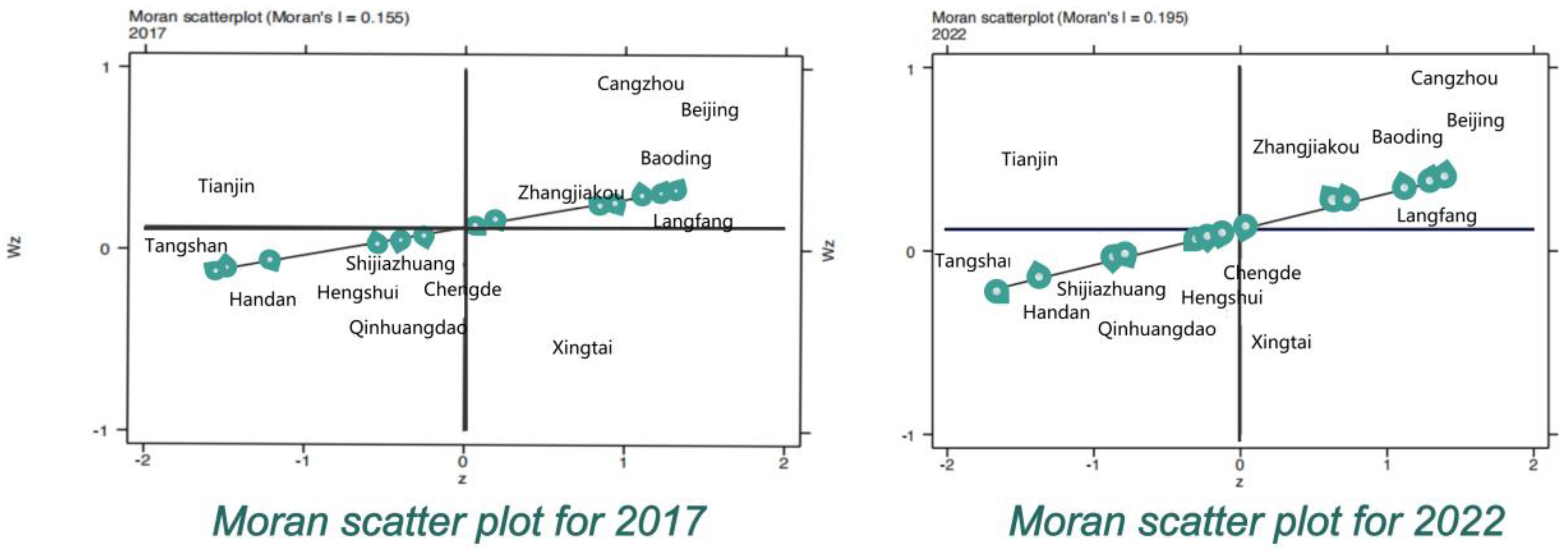
shows the calculation results of the global Moran index to verify whether it is spatially correlated. The average daily data for one year was taken as the calculation data for Moran’s index. Figure 3 is the Moran scatter plot, which visually shows the distribu-tion of AQI clusters in various cities and further explores the degree of spatial correlation in a specific area.

Table 4. Spatial transition of Moran scatter of urban AQI (2017~2022).

Cities	2017	2018	2019	2020	2021	2022
1	LL	LL	LL	LL	LL	LL
2	LL	LL	LL	HL	LL	LL
3	HH	HH	HH	HH	HH	HH
4	HL	HL	HL	HL	HL	HL
5	LL	LL	LL	LL	LL	LL
6	HH	HH	HH	HH	HH	HH
7	HH	HH	HH	HH	HH	HH
8	HH	HH	HH	HH	HL	HH
9	LH	LH	LH	LH	LH	LH
10	LL	LL	LL	LL	LL	LL
11	HH	HL	HH	HL	LL	HL
12	LL	LL	LL	LL	LL	LL
13	HH	HH	HH	HH	HH	HH

Note: HH: in the first quadrant, areas with high AQI are surrounded by other cities that also have high AQI; LH: in the second quadrant, areas with a low AQI are surrounded by other cities with a high AQI; LL: in the third quadrant, areas with a low AQI are surrounded by other cities with the same low AQI; HL: in the fourth quadrant, areas with a high AQI are surrounded by other cities with a low AQI.

shows the distribution trend of the Moran index, from which there is a temporal and spatial transfer process for the AQI.

Table 3 shows the AQI of thirteen cities in the Beijing-Tianjin-Hebei region from 2017 to 2022. It can be seen from the table that the Moran index has passed the 5% confidence test and is positive. The results showed that there was a positive spatial correlation, the AQI tended to be agglomerated in space, and the distribution of the air quality index was concentrated and encircled.

As shown in Figure 3, the Moran scatter plot set for each city’s AQI is distributed in the first and third quadrants, indicating a significant positive contribution of each city’s air quality in the local space. The total number of cities located in the 1,3-quadrant re-mained unchanged at 0.77 in the total sample. Most cities maintain similar cluster charac-teristics to their neighbors.

In addition, only three cities have experienced location migration of the Moran scat-tering point, namely, Chengde, Langfang, and Hengshui. Among them, Hengshui and Langfang return to their original spatial states after being influenced by the surrounding environment, while Cangzhou, which was at low air pollution, completely changes its original state and enters the HL region under the influence of high surrounding air pollu-tion. This indicates that the air quality of Chinese urban agglomerations is highly spatially correlated, that air pollution between urban agglomerations is interacting, and that the magnitude of the effect is not the same.

3.2.2. Local Gravitational Clustering

As described in Section 3.2.1, the AQI is spatially dependent. Non-independent air quality may affect clustered data with interdependent observations. Because the AQI is a comprehensive index, it can reflect the air quality of the city. Therefore, the daily AQI data of different cities are used as clustering variables to cluster cities.

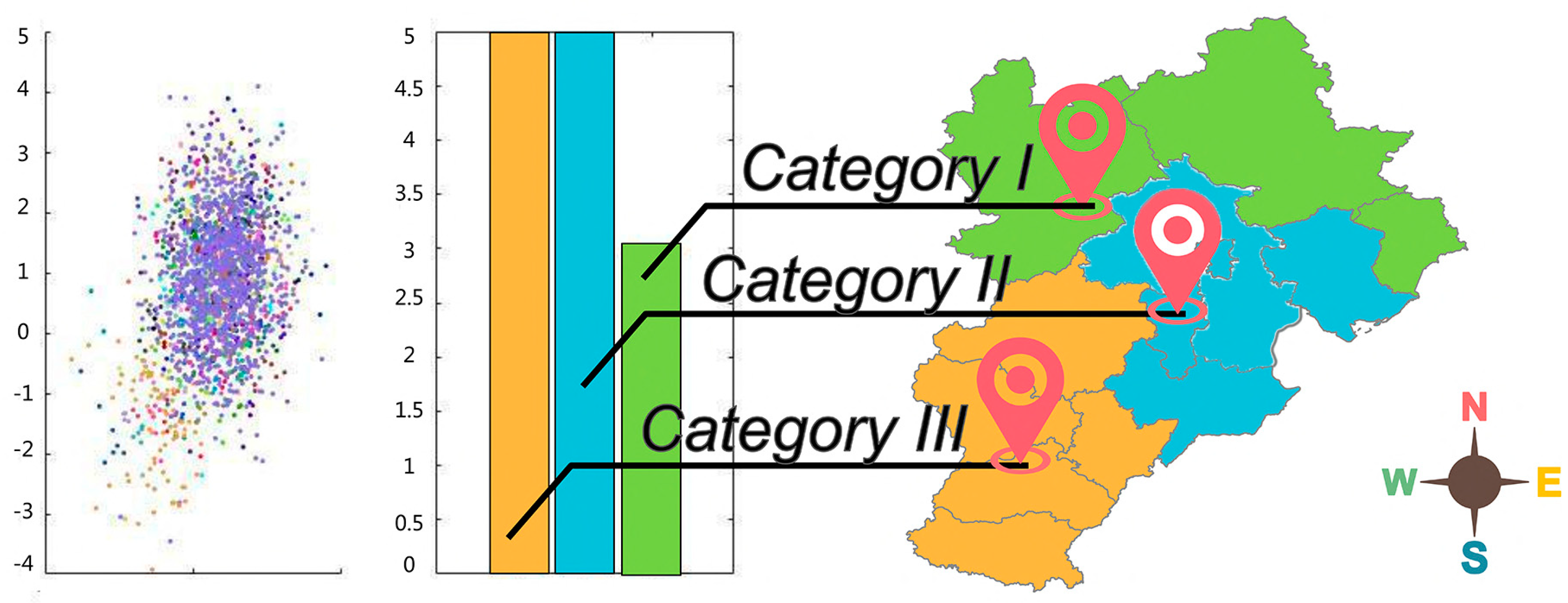
It can be seen from Figure 4 that the cities are divided into three different classes of air quality categories, showing good zonal differences and regional similarities.

Category I includes five cities: Shijiazhuang, Hengshui, Baoding, Xingtai, and Han-dan. This type of urban agglomeration is in the plains and has poor air pollution dispel-sion conditions. It is a heavy industrial city close to the inland, with many polluting industries superimposed on the transmission of air pollution from western Lu and north-ern Yu, where air pollution is most serious.

Category II includes five cities: Beijing, Cangzhou, Langfang, Tianjin, and Tangshan. Due to the large population and rapid economic development, in which the steel industry in Tangshan, coal in Cangzhou, and cement in Langfang were coupled, pollution is serious and air quality is deteriorating.

Category III includes three cities: Chengde, Qinhuangdao, and Zhangjiakou. Tour-ism-driven economic development, a few polluting industries, and mountainous terrain limit the flow and interaction of the atmosphere between the three cities and other cities, thus keeping air quality low.

Therefore, in order to continuously improve the environmental benefits and air qual-ity of the Beijing-Tianjin-Hebei region, the interaction between its cities cannot be ignored, and it is necessary to establish an improvement mechanism according to its geographical location, industrial structure, and economic development level to achieve the coordinated development of the Beijing-Tianjin-Hebei region.

3.3. Model Comparison Results

Based on the above experimental purposes, this section establishes three comparative experiments and uses the same evaluation index system to verify the forecasting performance.

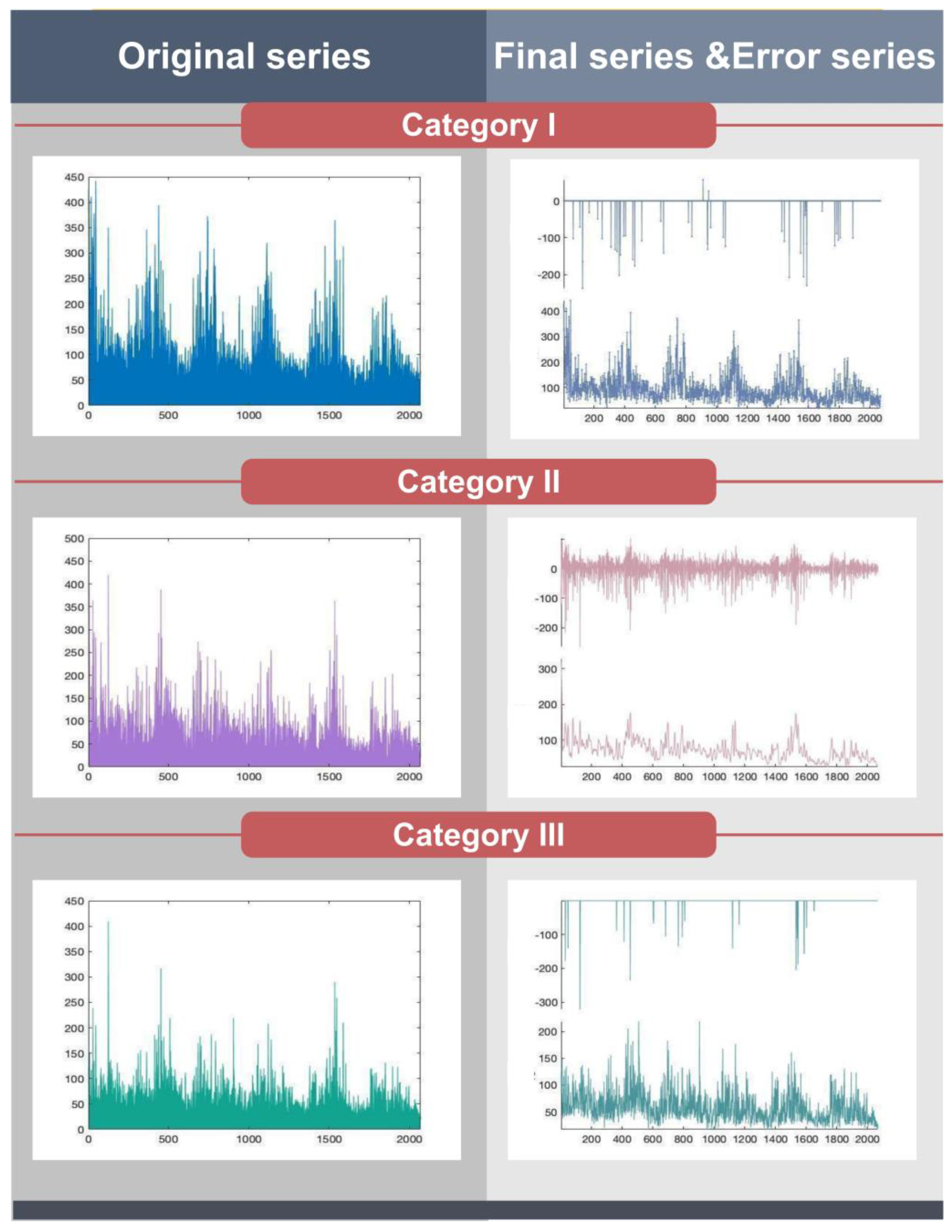
3.3.1. Feature Extraction Strategy

Due to the variability and nonlinearity of AQI in time series changes, it is difficult to accurately predict. In addition, there are many factors affecting air quality, including pol-icy factors, natural factors, etc., which are prone to fluctuations and singular values. Out-liers are data with significant deviations from most observations, which interfere with the training efficiency of the model. Removing outliers can improve forecasting accuracy. Therefore, before the experimental forecasting, it is necessary to test and correct the outli-ers of the data.

To illustrate the excellence of the optimized Hempel filtering in detecting and cor-recting outliers, comparative models based on different optimization algorithms were de-veloped, including the dragonfly algorithm (DA), SSA, and the honey badger algorithm (HBA). The comparison experiments were FCM and DHP-FCM, FCM and SHP-FCM, and FCM and HHP-FCM. The specific results are shown in

Table 5. Comparison of feature extraction strategies based on different optimization algorithms.

Cities	Method	MAPE	RMSE	MAE
Category I Beijing	FCM	25.54	25.15	17.76
	DHP-FCM	39.47	37.52	24.25
	SHP-FCM	25.12	26.34	17.79
	HHP-FCM	25.40	21.94	15.91
Category II Shijiazhuang	FCM	40.51	37.73	21.18
	DHP-FCM	31.96	24.38	15.43
	SHP-FCM	36.27	21.02	15.36
	HHP-FCM	36.25	21.08	15.40
Category III Chengde	FCM	29.50	20.66	14.25
	DHP-FCM	28.85	20.31	13.93
	SHP-FCM	27.78	19.22	13.29
	HHP-FCM	29.56	19.62	13.87

Note: HP: Hampel filtering; DHP: Hampel filtering optimized by dragonfly algorithm (DA); SHP: Hampel filtering optimized squirrel search algorithm (SSA); HHP: Hampel filtering optimized honey badger algorithm (HBA).

and Figure 5.

From Table 5, it can be seen that the SHP-FCM model has the best performance on MAPE, RMSE, and MAE compared to other optimization models for Category I, Category II, and Category III. In addition, the SSA algorithm has an outstanding advantage in find-ing the best model parameters to build a better hybrid model. In the three urban clusters, the MAPE metrics were reduced by 1.6%, 10.5%, and 5.8% compared to those optimized using the SSA algorithm. This finding has been confirmed in several application scenarios.

Remark 1.

SHP not only removes significantly deviated data and reduces interference with the model training rate, but also reduces data variability and preserves original features. Furthermore, from the residual sequence of the right diagram, it can be seen that the processed data and the original data only change slightly, and only the median substitution in the data pane is performed on the extreme data. Therefore, the data preprocessing in this paper will not cause information loss to the data.

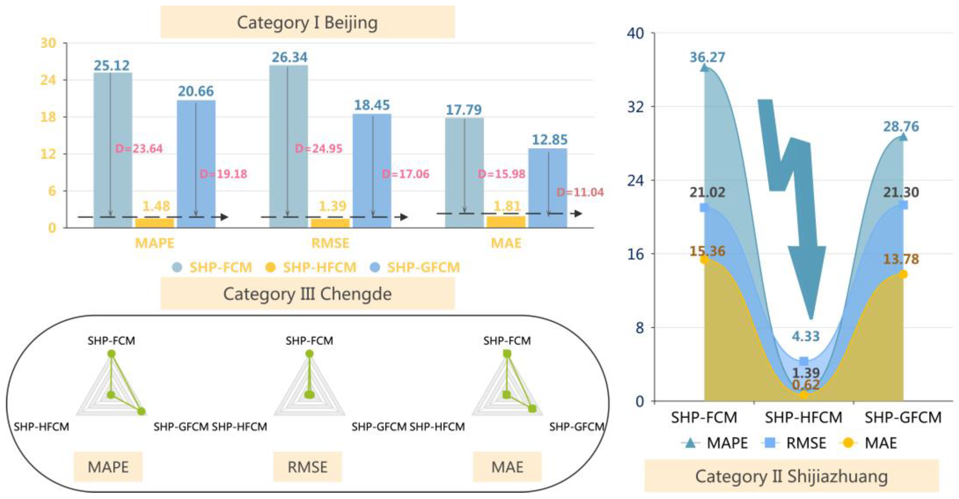
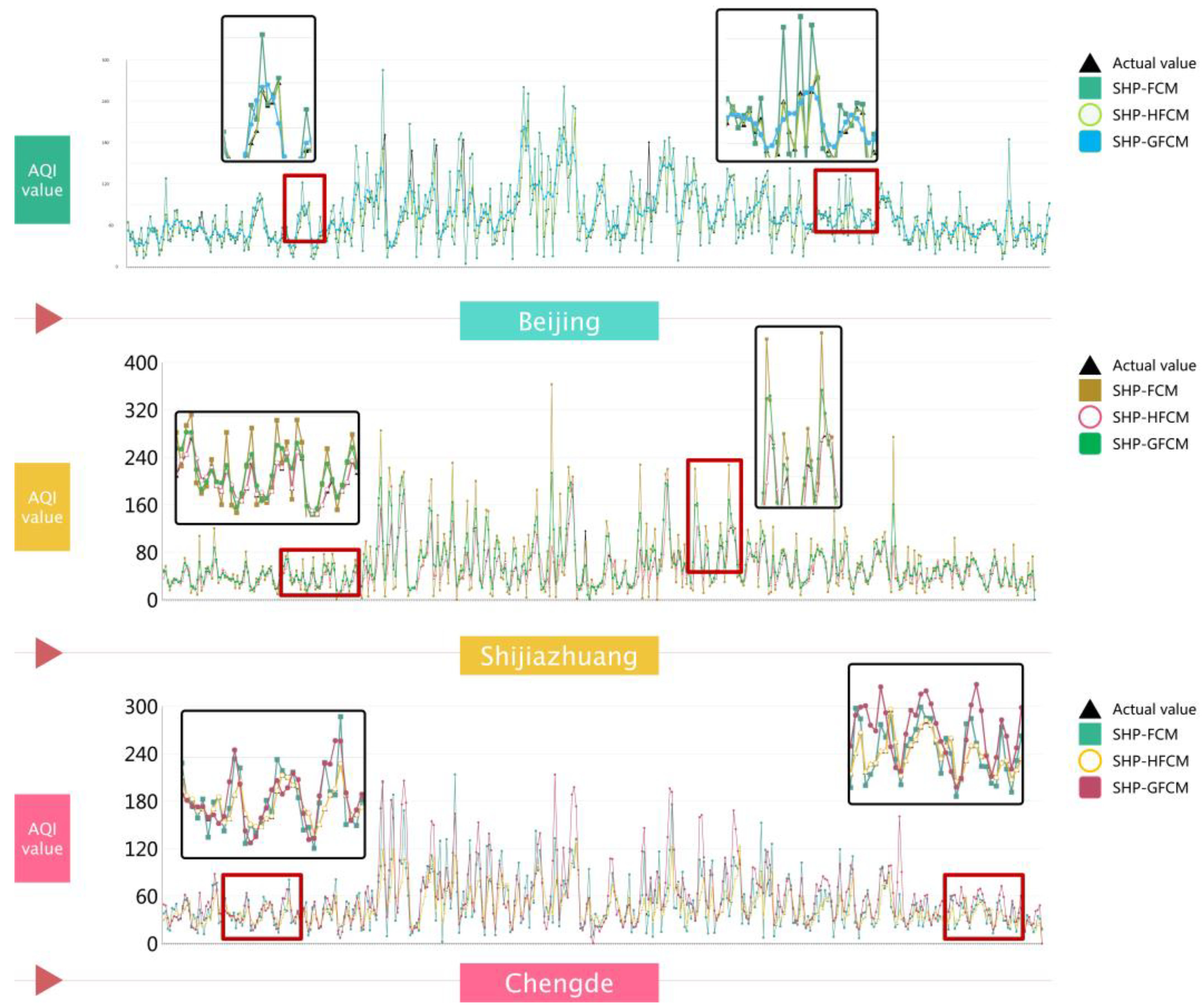
3.3.2. Probabilistic Hesitation Fuzzy Set Strategy

In the previous section, it was known that SHP is superior to DHP and HHP through comparative experiments. In the setting of SHP to extract data features, in order to verify the effectiveness of the HFCM prediction system constructed by combining the hesitant fuzzy information set strategy, FCM and Gaussian smooth fuzzy cognitive maps (GFCM) are also constructed for comparative experiments. The experimental results are shown in

Table 6. Comparison of forecasting effects based on different submodules of SHP.

Cities	Method	MAPE (%)	RMSE	MAE
Category I Beijing	SHP-FCM	25.12	26.34	17.79
	SHP-GFCM	20.66	18.45	12.85
	SHP-HFCM	1.48	1.39	1.81
Category II Shijiazhuang	SHP-FCM	36.27	21.02	15.36
	SHP-GFCM	28.76	21.30	13.78
	SHP-HFCM	1.12	4.33	0.69
Category III Chengde	SHP-FCM	27.78	19.22	13.29
	SHP-GFCM	24.14	1.11	9.75
	SHP-HFCM	0.49	0.62	0.23

Note: FCM: fuzzy cognitive maps; HFCM: hesitant fuzzy cognitive maps. GFCM: Gaussian smoothed fuzzy cognitive maps.

, Figure 6 and Figure 7.

The results in Table 6 showed that adaptive feature extraction using the Hampel fil-tering algorithm on the original data significantly improved forecasting accuracy com-pared to the direct use of fuzzy cognitive maps. In the comparison of the first type of model to improve the forecasting effect of the original single model, in the case of MAPE, the proposed model decreased by 94.1083% compared with FCM. And GFCM decreased by 17.7548% compared with FCM. In addition, MAE and RMSE also showed different degrees of improvement in each type of urban cluster. Taking Beijing as an example, SHP-FCM and SHP-GFCM are 24.95 and 17.06 higher than the RMSE of SHP-HFCM, respect-tively. The proposed model SHP-HFCM in Shijiazhuang has MAPE, RMSE, and MAE of 1.12%, 4.33, and 0.69, respectively, which are significantly less than the other two compar-ison models.

In particular, the third type of urban agglomeration has the best forecasting accuracy. In all evaluation indicators, the feature extraction strategy based on SHP is significantly better than the hybrid forecasting system based on ordinary fuzziness and Gaussian smoothing.

Remark 2.

HFCM has non-negligible advantages over FCM and GFCM in data forecasting. The proposed novel hesitant fuzzy cognitive maps can not only effectively eliminate uncertain infor-mation and unstable elements in time series but also be a promising method for processing the characteristics of time series forecast data itself.

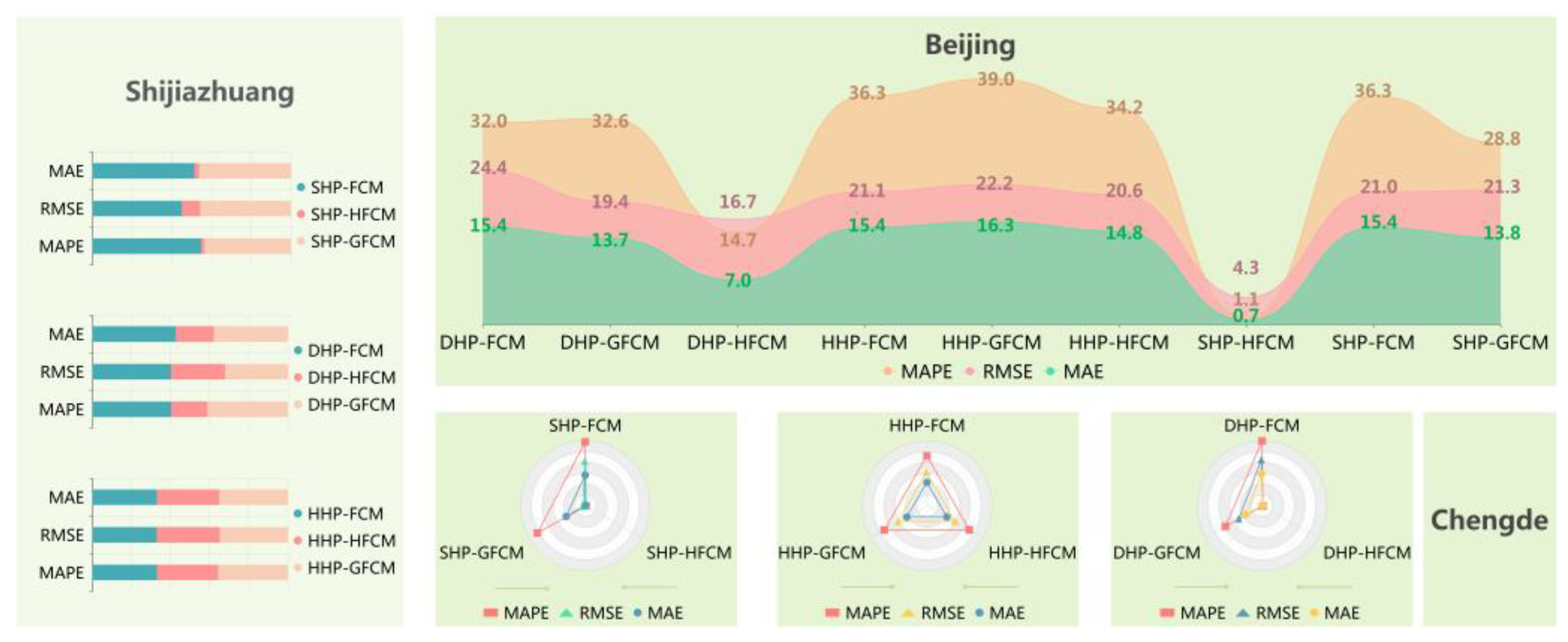
3.3.3. Comparison of Mixed Models in Different Data Preprocessing Environments

In addition, to show the scalability of hesitant, ambiguous information, the third comparison model is established. The FCM, HFCM, and GFCM data processing methods in the SHP, DHP, and HHP cases were compared. The results are shown in

Table 7. Comparison of hybrid models based on various feature extraction strategies.

Cities	Method	MAPE (%)	RMSE	MAE
Category I Beijing	DHP-FCM	39.47	37.52	24.25
	DHP-GFCM	30.21	26.19	18.98
	DHP-HFCM	21.45	21.74	13.48
	HHP-FCM	25.40	21.94	15.91
	HHP-GFCM	27.24	23.24	16.89
	HHP-HFCM	25.00	21.48	15.58
	SHP-FCM	25.12	26.34	17.79
	SHP-GFCM	20.66	18.45	12.85
	SHP-HFCM	1.48	1.39	1.81
Category II Shijiazhuang	DHP-FCM	31.96	24.38	15.43
	DHP-GFCM	32.64	19.40	13.66
	DHP-HFCM	14.66	16.72	7.01
	HHP-FCM	36.25	21.08	15.40
	HHP-GFCM	38.97	22.18	16.30
	HHP-HFCM	34.24	20.64	14.83
	SHP-FCM	36.27	21.02	15.36
	SHP-GFCM	28.76	21.30	13.78
	SHP-HFCM	1.12	4.33	0.69
Category III Chengde	DHP-FCM	28.85	20.31	13.93
	DHP-GFCM	18.67	11.87	8.38
	DHP-HFCM	0.53	0.47	0.25
	HHP-FCM	29.56	19.62	13.87
	HHP-GFCM	29.27	19.61	13.82
	HHP-HFCM	29.46	19.63	13.87
	SHP-FCM	27.78	19.22	13.29
	SHP-GFCM	24.14	1.11	9.75
	SHP-HFCM	0.49	0.62	0.23

and Figure 8.

Table 7 shows the performance indicator values for all submodules launched for the three considered environments. Especially taking the third type of urban agglomeration as an example, $SHP-HFC{M}_{Chengde}^{MAPE}=0.49$, $SHP-HFC{M}_{Chengde}^{RMSE}=0.62$, $SHP-HFC{M}_{Chengde}^{MAE}=0.23$, so for the same data preprocessing environment, the model using the HFCM method is better than the model using the FCM and the GFCM. In addition, the MAPE values for various hybrid forecasting systems are $SHP-HFC{M}_{Beijing}^{MAPE}=1.48$, $SHP-HFC{M}_{Shijiazhuang}^{MAPE}=1.12$, $SHP-HFC{M}_{Chengde}^{MAPE}=0.62$, thus it is concluded that SSA plays an important role in HFCM forecasting. After comprehensive comparison, the proposed model has a good effect in the forecasting of pollutant concentration series.

Remark 3.

In different data preprocessing scenarios, the submodule with the best predictive per-formance is uniquely identified. The hybrid forecasting system based on HFCM constructed in this paper achieves the best results of all evaluation indicators under different data processing environ-ments. This property has been demonstrated in three different scenarios.

4. Discussion

4.1. Robustness of the Proposed Model

The purpose of the robustness test is to investigate whether the daily data are non-stationary when the air quality receives the impact of high pollution. At this time, whether the model can still work normally and whether the forecasting accuracy fluctuates greatly are evaluated in this test. In this experiment, the data of the training set increases the ran-dom number in the range of (−2, 2), which is considered to be from random interference; then, observe the changes of each performance index; the comparison results are shown in

Table 8. The results of robustness test.

	MAPE (%)			RMSE			MAE
	Random	Proposed	Change	Random	Proposed	Change	Random	Proposed	Change
Beijing
FCM	32.15	25.54	6.61	30.15	25.15	5.00	20.26	17.76	2.5
SHP-FCM	30.72	25.12	5.6	28.61	26.34	2.27	19.89	17.79	2.1
SHP-HFCM	1.39	1.48	0.09	1.58	1.39	0.19	1.76	1.81	0.05
Mean	21.42	17.38	4.04	20.11	17.63	2.49	13.97	12.45	1.52
Std	17.36	13.77	3.59	16.07	14.07	1.99	10.58	9.22	1.36
Shijiazhuang
FCM	45.49	40.51	4.98	28.28	37.73	9.45	19.63	21.18	1.55
SHP-FCM	45.71	36.27	9.44	28.16	21.02	7.14	19.57	15.36	4.21
SHP-HFCM	0.83	1.12	0.29	4.17	4.33	0.16	0.52	0.69	0.17
Mean	30.68	25.97	4.71	20.20	21.03	0.82	13.24	12.41	0.83
Std	25.85	21.62	4.23	13.89	16.70	2.81	11.02	10.56	0.46
Chengde
FCM	32.26	29.50	2.76	20.34	20.66	0.32	13.81	14.25	0.44
SHP-FCM	32.04	27.78	4.26	20.55	19.22	1.33	13.98	13.29	0.69
SHP-HFCM	0.67	0.49	0.18	0.50	0.62	0.12	0.31	0.23	0.08
Mean	21.66	19.26	2.40	13.80	13.50	0.30	9.37	9.26	0.11
Std	18.18	16.28	1.90	11.52	11.18	0.34	7.84	7.83	0.01

Note: Random represents adding random disturbance to simulate air situation. Proposed represents the original data. Change is the absolute value of the difference between the data after adding the disturbance and the accuracy data model, that is, the magnitude of the change.

.

Before and after adding random disturbance, the MAPE values of Beijing were 1.39% and 1.48%, respectively; only 0.09% changed, and the same was true for other cities. After adding random disturbances, the forecasting accuracy of the proposed model changed slightly: Shijiazhuang changed by 0.29%, and Chengde changed by 0.18%. It can also be seen from Table 7 that the average RMSE of the three observation cities of the original data model is 17.63, 21.03, and 13.50, respectively. Compared with the model with increased disturbance, the values of MAPE change by 2.49, 0.82, and 0.3, respectively, which clarifies that the random disturbance will not affect the forecasting performance. In addition, for the original data model, taking the predicted value of Beijing as an example, the average MAE is 12.45, and the standard deviation is 9.22. From the model, after increasing the disturbance, the average MAE increases slightly, the standard deviation increases to 13.97, the change range is 1.52, and the standard deviation change range is 1.36, which indicates that the random disturbance is not significant.

In summary, by observing the fluctuation of the forecasting results of each city, the forecasting performance of the model proposed in this paper has not changed significantly and still maintains an outstanding forecasting effect. Therefore, there is enough evidence to prove that although the air quality will be affected by other factors, such as high pollu-tion or other abnormal conditions, the proposed model can still have stability.

4.2. Differences of the Proposed Model

The discrepancy test of the forecasting system proposed in this paper will be further discussed in this section. To test whether the forecasting performance of the proposed hybrid forecasting model is significantly different from other forecasting models, the DM test and the MDM test are used to perform statistical tests.

From the experimental results in

Table 9. The results of testing model differences.

Category	Method	DM	P	MDM	P
Category I Beijing	DHP-FCM	15.2192	8.39 × 10−42	15.2007	1.01 × 10−41
	DHP-GFCM	9.7186	3.11 × 10−20	9.7068	3.42 × 10−20
	DHP-HFCM	8.0531	3.88 × 10−25	8.0423	2.63 × 10−25
	HHP-FCM	13.6566	2.83 × 10−35	13.6401	3.31 × 10−35
	HHP-GFCM	5.8835	8.34 × 10−9	5.8764	8.67 × 10−9
	HHP-HFCM	5.1544	3.26 × 10−7	5.1478	3.19 × 10−7
	SHP-FCM	5.7104	2.16 × 10−8	5.7034	2.25 × 10−8
	SHP-GFCM	6.4946	2.41 × 10−10	6.4867	2.52 × 10−10
Category II Shijiazhuang	DHP-FCM	16.4863	3.10 × 10−47	16.4663	3.78 × 10−47
	DHP-GFCM	10.0901	1.55 × 10−21	10.0778	1.71 × 10−21
	DHP-HFCM	5.9216	8.34 × 10−11	5.9148	8.34 × 10−11
	HHP-FCM	15.9536	6.12 × 10−45	15.9342	7.42 × 10−45
	HHP-GFCM	9.5553	1.14 × 10−19	9.5437	1.25 × 10−19
	HHP-HFCM	9.1332	1.25 × 10−13	9.1277	1.36 × 10−13
	SHP-FCM	10.5755	2.79 × 10−23	10.5626	3.11 × 10−23
	SHP-GFCM	11.6521	2.63 × 10−27	11.6380	2.98 × 10−27
Category III Chengde	DHP-FCM	13.0401	4.63 × 10−41	13.0242	5.54 × 10−41
	DHP-GFCM	12.9219	8.93 × 10−34	12.9062	1.04 × 10−33
	DHP-HFCM	1.4234	3.74 × 10−51	1.4217	4.62 × 10−51
	HHP-FCM	10.3126	4.40 × 10−43	10.3001	5.30 × 10−43
	HHP-GFCM	10.2920	1.39 × 10−39	10.2795	1.65 × 10−39
	HHP-HFCM	10.3339	2.25 × 10−36	10.3214	2.64 × 10−36
	SHP-FCM	13.4234	9.09 × 10−33	13.4071	1.05 × 10−32
	SHP-GFCM	13.2622	2.72 × 10−32	13.2461	3.14 × 10−32

Note: The model SHP-HFCM proposed in this study is used for comparison with the above combinatorial strategy, where the statistic p-value represents the probability.

, the loss series of the proposed hybrid fore-casting system passed the significance test at the 5% confidence level. It denotes that the proposed hybrid forecasting system has higher forecasting efficiency than other hybrid strategies, and it is not a coincidence that the forecasting is significantly different.

Compared with other models, the model proposed in this paper has the best results in any possible data environment. On the one hand, it performs spatial effect analysis and data feature extraction before data forecasting, which can better utilize the spatial and data features of the data for subsequent forecasting, and this is the excellence of the model. On the other hand, the system continuously updates the output conceptual values after k iterations by combining the geographic location of each data and does not directly output the forecasting results, but it eliminates the uniqueness of the data itself through fuzzy time series, and the forecasting results are more superior.

4.3. Application of the Proposed Model

The proposed model not only has outstanding forecasting performance but also has potential functions in practical applications. The early warning system consists of three modules: spatial feature analysis module, data preprocessing module, and fuzzy infor-mation prediction module. The following analyzes its practical significance from these three modules.

• Air pollution has spatial spillover effects, so the spatial feature analysis module can comprehensively consider the interaction of urban agglomerations. In addition, it also provides theoretical support for the formulation of pollution control policies among urban agglomerations and facilitates coordinated governance among urban agglomerations.
• In fact, air quality is affected by many factors, including information ambiguity and uncertainty. Through the data preprocessing module, it can remove the outliers and noise from the data, making the data features more obvious and achieving better forecasting performance.
• Accurate AQI forecasting results can provide early warning information for actual life and production activities. From the perspective of the public, the forecasting of air quality can let the public understand the air quality, the scope of air quality dete-rioration, the degree of deterioration, and the development trend; secondly, it guides the daily activities and behaviors of residents, protects the physical and mental health of the people, and reduces the incidence of diseases. From the perspective of social economy, it can not only provide the theoretical basis for pollution control measures, such as strict control of motor vehicle pollution, reduction of coal consumption, shut-down of polluting enterprises, control of construction sites and road dust, and super-vision of factories with large pollutant emissions.

5. Conclusions

In terms of application, it is profoundly important to make accurate forecasts of air quality. The air environment is an important guarantee for people’s health and production safety, and understanding real-time AQI can provide a theoretical basis for establishing an early warning system on the one hand, and a tool for implementing pollution control policies on the other. However, because AQI has the complexity and nonlinearity of time series changes, and has spatial correlation among urban clusters, it is difficult to make accurate forecasting. Coupled with the fact that it is influenced by many factors and prone to fluctuations and singular values, it is even more challenging for the forecasting effect of the model. Therefore, this paper proposes a novel spatiotemporal hybrid forecasting system to realize the time series forecasting of AQI. Three comparative experiments were established using the air quality indices of thirteen cities in the Beijing-Tianjin-Hebei re-gion of China to analyze and demonstrate, and the results are as follows:

• First, the spatial feature extraction module is built. The module successfully extracted the spatial overflow features, captured the dynamic transition of air quality, and per-formed cluster analysis with different sizes and weights for irregular data.
• The adaptive Hampel filtering model improved by SSA is the best data processing sub-module for comparison with FCM, DHP-FCM, and HHP-FCM.
• The first proposed HFCM forecasting model plays an irreplaceable role in time series forecasting in the same data preprocessing environment. The model reduced MAPE by 94.1083%, 96.9120%, and 98.2361% for three different urban clusters.
• In the environment of different data preprocessing methods, the model proposed in this paper can still make accurate forecasts for data with large fluctuations and mu-tations. MAPE, RMSE, and MAE reach the minimum values in the three urban ag-glomerations.

In summary, the proposed air quality forecasting system has outstanding forecasting performance in handling low-quality and large-noise data. Although the model makes an accurate prediction by analyzing the spatial correlation between the target city and the adjacent city and excavating its internal relationship, this study also has shortcomings, and the stability needs to be improved when optimizing the Hampel parameter values for single objectives. In future research, we can consider a multi-objective optimization algorithm and select other urban agglomerations for research to further verify the superiority of the forecasting model proposed in this paper for air quality index forecasting.