The Intersectoral Systemic Risk Shock of Emergency Crisis Events in China’s Financial Market: Nonparametric Methods and Panel Event Study Analyses

Abstract

By employing two systemic risk methods, the marginal expected shortfall (MES) and the component expected shortfall (CES), this paper measures the systemic risk level of all sectors in China’s financial market from 2014 to 2022; thereby, it researches the total effect of sectoral systemic risk using a panel event study model during the three main emergency crisis events. Moreover, two nonparametric methods are utilized, the Wilcoxon signed rank sum test and the bootstrap Kolmogorov–Smirnov test, in order to investigate the changes in individual effects and the dominant ranks of sectoral systemic risk. The empirical results show that (1) the mean values and volatilities of CES and MES of all sectors have a higher level of magnitude in the extreme risk status than those in the normal risk status; (2) by comparing the total effects of three crisis events, we find that different from the continuous shock effect caused by two other events, sectoral systemic risk has a hysteresis effect on the entire market after the outbreak of COVID-19; (3) the long-term and short-term individual effects of sectoral systemic risk in all sectors are different from each other during three events; and (4) the dominance tests of MES are more sensitive and thus better demonstrate the changes in the rankings of sectoral systemic risk than the dominant tests of CES during the emergency crisis events.

1. Introduction

Emergency crisis events often arouse a series of financial market fluctuations and catalyze a revolution in financial stability supervision [1]. The most typical case is the bankruptcy of US financial institutions in 2008, which triggered a tremendous systemic risk in the global financial system. Since then, the financial regulator has been strengthening the detection and prevention of systemic risk under the emergency market situation. Over the last ten years, China’s financial market has experienced three main systemic risk shocks due to the occurrence of crisis events, such as 2015’s A-share market crash, 2018’s Sino–US trade friction and 2020’s COVID-19 pandemic [2]. These crisis events, also called black swan events, heavily interfere with sound and sustainable financial market development, and cause systemic risk shock across different industries. The amplification of financial shock eventually evolves into a crisis across the entire system because of the interconnected relationship of each economic sector. Therefore, it is essential to measure the negative effects of systemic risk more accurately in every sector and capture the differences in the systemic risk rank level between them in the various contexts of emergency crisis events.

Some researchers have discussed the impact of these abnormal events on China’s financial market from various perspectives, such as financial networks and risk contagion [3,4]. The Chinese A-share market went through an intensive fluctuation period in 2015, and the Shanghai Composite Index experienced an extreme plummet and systematic meltdown [5]. Fang et al. (2018) found that financial institutions’ idiosyncratic risk can be affected by their connectedness with other firms, which significantly increased during the Chinese stock market crash in June 2015 [6]. Xu and Gao (2019) employed nonlinear causality tests and dynamic copula methods to explore the degree of financial risk contagion in the stock market and found that the lower tail dependence coefficients of the Chinese stock market were remarkably amplified after the occurrence of the A-share market crash [7]. The Sino–US trade friction in 2018 also had a serious degree of impact on China’s financial market, which spread across the overall financial system. Li et al. (2020) suggest that China’s stock market’s ability to maintain stability was weak when some weighted stocks abnormally fluctuated or suffered targeted shocks during the Sino–US trade friction [8]. In addition, 2020’s COVID-19 pandemic, as an emergency public health event, led to a rise in pessimistic expectations about economic recession, which exacerbated the downward trend in the financial market [9]. Consequently, these three unexpected crisis events brought new challenges to market supervision and risk control in the Chinese financial system.

Undoubtedly, this type of intersectoral financial risk agglomeration can develop as a profound systemic risk among all sectors in the entire market during black swan events. Grundke and Tuchscherer (2018) explore the institution’s systemic risk level change and its forecasting power for crisis events, and analyze the informational value of systemic risk measures for predicting the extent and the speed of these events [10]. Avramidis and Pasiouras (2015) give evidence of extreme event dependence on financial institutions’ systemic risk capital and propose a factor model that accounts for them [11]. Based on the daily closing price of China’s A-share market, Huang et al. (2022) constructed dynamic weighted networks and extracted the logistic slope as the characteristic indicator of the network structure in order to detect the influences of crisis events, including 2015’s A-share market crash, 2018’s Sino–US trade friction and 2020’s COVID-19 pandemic [2]. Recently, many researchers have focused more on the shock impacts of the COVID-19 outbreak on financial risk contagions, including Zhang et al. (2020) [12], Guo et al. (2021) [13], and Samitas et al. (2022) [14]. After the occurrence of this unprecedented public health crisis event, the systemic risk surged and stagnated at an elevated level, which put the whole financial market under high strain [15,16]. The COVID-19 pandemic intensified the total risk connectedness of financial networks and then created a sharp increase in the intensity of systemic risk [17,18,19]. However, this group of studies pays little attention to exploring the sectoral systemic risk shock of emergency crisis events when comparing the heterogenous individual effects across different industries.

Motivated by the above realistic situations and related works, we address the key aims of this study as follows: (1) Measure the systemic risk level of all sectors in China’s financial market more comprehensively and accurately, especially during the financial turmoil periods. (2) Explore the different situations in terms of the total effects on sectoral systemic risk based on three various crisis events in China’s financial market. (3) Capture the variations in the individual effects of sectoral systemic risk in order to compare the reactions of all entity sectors to these crisis events. (4) Construct the dominant order of systemic risk among all sectors to illustrate the relative position of each one in the various systemic risk connections during crisis events. More specifically, by employing the two measures of systemic risk, the component expected shortfall (CES) and the marginal expected shortfall (MES), this paper empirically researches the differences in the average effects and total effects of sectoral systemic risk in China’s financial market using a panel event study model between the periods of three main black swan events: the deleveraging policy implementation of the A-share market in 2015, the announcement of the US placing additional trade tariffs on China’s goods in 2018 and the COVID-19 outbreak in 2020. Moreover, two nonparametric methods are utilized, the Wilcoxon signed rank sum test and the bootstrap Kolmogorov–Smirnov test, to investigate the change level in individual effects and the dominant orders of sectoral systemic risk in different industries during black swan events. Figure 1 is the theoretical diagram of this paper.

This study is an effective complement to the regulation and measurement of systemic risk in different sectors in regard to the stability of China’s financial market during black swan events. Generally, we are more focused on the total effects and the individual effects of sectoral systemic risk caused by the emergency crisis events, and particularly, the shifts in the systemic risk dominant orders of all sectors during the pre-event and post-event periods of emergency crises. Our main findings are as follows: First, the mean values and volatilities of CES and MES of all sectors have a higher level of magnitude in the extreme risk situation than those in the normal risk case, indicating that each financial sector is systemically relevant and significantly contributes to the overall market. Second, by comparing the total effects of three crisis events, we find that compared to the continuous shock caused by two other events to the overall systemic risk in the entire market from the aspect of all sectors, sectoral systemic risk has a hysteresis effect on the entire market after the COVID-19 outbreak. Third, the long-term and short-term individual effects of sectoral systemic risk in all sectors of the three emergency crisis events are different from each other, due to the different characteristics of events, depending possibly on the most affected industries and their risk degrees. Fourth, the dominant orders of systemic risk level can clearly present the net spill-in and the net spill-out sectors, and the dominance tests of marginal expected shortfall (MES) are more sensitive; they can thus more effectively demonstrate the changes in the rankings of sectoral systemic risk than the dominant tests of component expected shortfall (CES) during the emergency crisis events.

The first contribution of this paper to the existing literature is that we measure the sectoral systemic risk by employing the CES and MES, which enables us to extend the research on the impacts of the black swan events on different sectors into the sectoral systemic risk level in China’s financial market. Much research has concentrated the study of the stock return’s shock effect and the volatility correlation between sectors during the pandemic, but most of it ignores the overall risk effect that every single sector has on the entire market [20,21]. Costa et al. (2022) examine the volatility connectedness and the changes in the pairwise connections of sectoral indices in the US stock market [22]. Choi (2022) observes the enhanced volatility spillovers and the contagion effects among various industries during the COVID-19 pandemic [23]. Alomari et al. (2022) employ quantile regression to analyze the relationship between changes in the newspaper-based infectious diseases tracking index and sectoral stock market returns [24]. Nguyen (2022) examines the early impacts of the COVID-19 outbreak on the stock returns of 11 sectors using firm-level stock price data from 10 countries [25]. In contrast with these studies above, following the methods that are proposed by Acharya et al. (2012) [26] and Banulescu and Dumitrescu (2015) [27], we can more comprehensively detect the overall risk connections between the entire market and different sectors during financial turbulences, that is, the systemic risk of all sectors both from the aspects of absolute contribution and marginal contribution.

Another contribution of our study is that we consider the dynamic variation in the coefficients of the event variables around the baseline time of the crisis event, which allows a clear visual representation of the shock of the crisis event on sectoral systemic risk and its temporal trend in the total effect. Different from using the basic event study method to analyze the influences of the COVID-19 pandemic on different sectors, such as that used by Harjoto et al. (2020) [28], He et al. (2020) [29], and Liu et al. (2021) [30], we employ the panel event study model with two fixed effects by referring to Freyaldenhoven et al. (2019) [31]; this in order to obtain the time-varying coefficients of the event’s lead and lag variables at each time point more precisely. Unlike Ouyang et al. (2022) [32], our model contains the full setting of posterior period variables that can detect the dynamic nature of the impact of the COVID-19 pandemic on sectoral systemic risk over time, whether it is transitory or perennial [33]. In addition, we not only discuss the change in systemic risk during the crisis within the limits of a single industry, like Tian et al. (2022) [34], Shahzad et al. (2022) [35], and Zou and Wang (2022) [36] do, but also explore the total effect of the systemic risk that was introduced by the COVID-19 outbreak into all sectors on the financial market and the difference in its reaction to two other crisis events: the implementation of the A-share market deleveraging policy in 2015 and the announcement of the US’s additional trade tariffs in 2018.

Lastly, we evaluate the differences in individual effects due to the pandemic and the dominant order of sectoral systemic risk, which helps us to detect those sectors important to the entire market in terms of systemic risk contribution and shifts in the systemic risk dominant order of each sector during the crisis and non-crisis periods. Similar to the applications of the Wilcoxon signed rank sum test by Ahnert and Georg (2018) [37] and Morelli and Vioto (2020) [38], we use this measure to test the distinctions made clear in the systemic risk level of each sector between the pre-event and post-event periods, and compare these sorts of individual effects during the three crisis events covered by our sample period. Moreover, in line with Bernal et al. (2014) [39] and Wen et al. (2020) [40], we employ another nonparametric method, the bootstrap Kolmogorov–Smirnov test, in order to estimate the dominant relationships of systemic risk between different sectors. The existing studies fail to explicitly consider the overall contribution rank of systemic risk in different sectors, but we furtherly identify the dominant role of each sector using others both in the systemic risk fields of CES and MES. Therefore, to bridge this research gap, this paper takes the COVID-19 outbreak as an example, and clearly illustrates the changes in the dominant ranks and connections of sectoral systemic risk caused by the emergency crisis events from the all-sector-level perspective.

The remainder of the paper is organized as follows. In Section 2, we develop the specification and estimation framework, and present the data and variables included in the empirical models. Section 3 discusses the results and analysis, and Section 4 concludes the paper with some financial supervision and investment implications.

2. Methodology and Estimation Framework

2.1. Specification of Sectoral Systemic Risk

To measure the level of sectoral systemic risk in China’s financial market, we employ the Marginal Expected Shortfall approach, which derives from the concept of the Expected Shortfall. As argued by Acharya et al. (2012) [26], the measure of MES can reflect the sensitivity of the total risk of the entire system to a unit change in one institution or industry in the financial system. Considering a financial market contains $n$ sectors, $r_{m,t}={{\displaystyle \sum }}_{i=1}^n{\omega }_{i,t}{r}_{i,t}$ denotes the aggregate return of the whole system at time $t$, $r_{i,t}$ is the corresponding return of sector $i$, and ${\omega }_{i,t}$ is the related weight of the market size of each sector within the system at time $t$. First, the Expected Shortfall is defined as follows:

$${\mathrm{ES}}_{\mathrm{m},\mathrm{t}-1}\left(C\right)=-{\mathrm{E}}_{\mathrm{t}-1}\left(r_{m,t}|r_{m,t}<C\right)$$

(1)

where $C$ is a known threshold to denote the loss condition of the distress event. It is usually measured by the Value-at-Risk (VaR) at a given confidence level. Then, the MES corresponds to the marginal contribution of an institution or industry to the total risk of the financial system measured by ES, which is defined as follows:

$${\mathrm{MES}}_{\mathrm{i},\mathrm{t}}\left(C\right)=\frac{\partial {\mathrm{ES}}_{\mathrm{m},\mathrm{t}-1}\left(C\right)}{\partial {\mathsf{\omega }}_{\mathrm{i},\mathrm{t}}}=-{\mathrm{E}}_{\mathrm{t}-1}\left(r_{i,t}|r_{m,t}<C\right)$$

(2)

Based on the definition of MES, the Component Expected Shortfall, proposed by Banulescu and Dumitrescu (2015) [27], is a measure of the absolute contribution of systemic risk. Compared with Equation (2), the CES is also defined as part of the ES of the entire system due to the sector $i$, which is given as follows:

$${\mathrm{CES}}_{\mathrm{i},\mathrm{t}}\left(C\right)={\mathsf{\omega }}_{\mathrm{i},\mathrm{t}}\frac{\partial {\mathrm{ES}}_{\mathrm{m},\mathrm{t}-1}\left(C\right)}{\partial {\mathsf{\omega }}_{\mathrm{i},\mathrm{t}}}=-{\mathsf{\omega }}_{\mathrm{i},\mathrm{t}}{\mathrm{E}}_{\mathrm{t}-1}\left(r_{i,t}|r_{m,t}<C\right)$$

(3)

It is noticed that CES is measured by the product of MES and the weight of the sector, which represents the absolute contribution of sector $i$ to the risk of the financial system. In addition, the sum of all the sector’s CES is equal to the ES of the system: ${\mathrm{ES}}_{\mathrm{m},\mathrm{t}-1}\left(C\right)={{\displaystyle \sum }}_{\mathrm{i}=1}^{\mathrm{n}}{\mathrm{CES}}_{i,t}\left(C\right)$. It can be expressed as a percentage of ES, which denotes the proportion of systemic risk due to sector $i$ at time $t$. Consequently, the ${CES\%}_{i,t}\left(C\right)$ is given as follows:

$${\mathrm{CES}\%}_{\mathrm{i},\mathrm{t}}\left(C\right)=\frac{{\mathrm{CES}}_{\mathrm{I},\mathrm{t}}\left(C\right)}{{\mathrm{ES}}_{\mathrm{m},\mathrm{t}-1}\left(C\right)}\times 100\%=\frac{{\mathsf{\omega }}_{\mathrm{i},\mathrm{t}}{\mathrm{E}}_{\mathrm{t}-1}\left(r_{i,t}|r_{m,t}<C\right)}{{{\displaystyle \sum }}_{\mathrm{i}=1}^{\mathrm{n}}{\mathsf{\omega }}_{\mathrm{i},\mathrm{t}}{\mathrm{E}}_{\mathrm{t}-1}\left(r_{i,t}|r_{m,t}<C\right)}\times 100\%$$

(4)

2.2. Estimation Framework of Sectoral Systemic Risk

The estimation framework of MES and CES is mainly composed of three steps. First, by using a dynamic conditional correlation (DCC) model (Engle, 2002 [41]) combined with a GJR-GARCH (1,1) framework (Glosten et al., 1993 [42]), we obtain the conditional volatilities and standardized residuals for the market and sectors; this is in order to capture the time-varying correlations of couples of the entire market and each sectors. The derivation of the DCC-GJR-GARCH (1,1) model is presented as follows:

$$r_{i,t}={\mu }_{i,t}+{\epsilon }_{i,t}, r_{m,t}={\mu }_{m,t}+{\epsilon }_{m,t}$$

(5)

$${\sigma }_{i,t}^2={\eta }_{i,0}+{\eta }_{i,1}{\epsilon }_{i,t-1}^2+{\eta }_{i,2}{\sigma }_{i,t-1}^2+{\delta }_i{I}_{i,t-1}{\epsilon }_{i,t-1}^2$$

(6)

$${\sigma }_{m,t}^2={\eta }_{i,0}+{\eta }_{i,1}{\epsilon }_{m,t-1}^2+{\eta }_{i,2}{\sigma }_{m,t-1}^2+{\delta }_i{I}_{m,t-1}{\epsilon }_{m,t-1}^2$$

(7)

$${\sigma }_{im,t}=\left({\rho }_{im,t}+{\lambda }_i{I}_{m,t-1}\right){\sigma }_{i,t}{\sigma }_{m,t}$$

(8)

where e $r_{m,t}$ and $r_{i,t}$ denote the returns of the indices of the market and its sectors at time $t$; ${\mu }_{m,t}$ and ${\mu }_{i,t}$ are the conditional means; ${\sigma }_{i,t}^2$ and ${\sigma }_{m,t}^2$ are the conditional variances that follow a GARCH (1,1) specification and have the asymmetric volatility responses ${\delta }_i{I}_{i,t-1}{\epsilon }_{i,t-1}^2$ and ${\delta }_i{I}_{m,t-1}{\epsilon }_{m,t-1}^2$ to positive and negative shocks in Equations (6) and (7); and $I_{i,t-1}$ and $I_{m,t-1}$ are the dummy variables that take the value of one if ${\epsilon }_{i,t-1}<0$ or ${\epsilon }_{m,t-1}<0$, otherwise zero. Further, Equation (8) presents the process of the time-varying covariance ${\sigma }_{im,t}$, which is also considered the asymmetrical effect ${\lambda }_i{I}_{m,t-1}$ during the period of market decline. As developed by Engle (2016) [43], ${\rho }_{im,t}$ is the dynamic conditional correlation between the market and sectoral returns, and $q_{im,t}$ is the conditional covariance of the standardized residuals, which are shown as follows:

$${\rho }_{im,t}=\frac{q_{im,t}}{\sqrt{q_{ii,t}{q}_{mm,t}}}$$

(9)

$$q_{im,t}={\overline{\rho }}_{im}+\gamma \left(z_{i,t-1}{z}_{m,t-1}-{\overline{\rho }}_{im}\right)+\theta \left(q_{im,t-1}-{\overline{\rho }}_{im}\right)$$

(10)

where $q_{ii,t}$ and $q_{mm,t}$ are the conditional variances of the market and sectoral standardized residuals at time $t$; ${\overline{\rho }}_{im}$ is the constant unconditional covariance between the market and sectoral returns; and $z_{i,t-1}={\epsilon }_{i,t-1}/{\sigma }_{i,t-1}$ and $z_{m,t-1}={\epsilon }_{m,t-1}/{\sigma }_{m,t-1}$ are the standardized residuals of the sectoral and market returns. The coefficients $\gamma$ and $\theta$ in Equation (10) measure the effects of any previous shocks and conditional correlations on the current dynamic conditional correlations, and the correlation between the market and sectoral returns equal to the unconditional level ${\overline{\rho }}_{im}$ when $\gamma +\theta <1$. Therefore, we can obtain the estimation coefficients of the time-varying conditional correlation of each market and sector pair.

Second, based on the estimation framework of dynamic conditional correlation, we can extend the expressions of MES and CES into Equations (2) and (3), as follows:

$$ME{S}_{i,t}\left(C\right)={\sigma }_{i,t}{\rho }_{im,t}{\mathrm{E}}_{\mathrm{t}-1}\left({\epsilon }_{m,t}|{\epsilon }_{m,t}<\frac{C}{{\sigma }_{m,t}}\right)+{\sigma }_{i,t}\sqrt{1-{\rho }_{im,t}^2}{\mathrm{E}}_{\mathrm{t}-1}\left({\xi }_{i,t}|{\epsilon }_{m,t}<\frac{C}{{\sigma }_{m,t}}\right)$$

(11)

$$CE{S}_{i,t}\left(C\right)=-{\omega }_{i,t}\left[{\sigma }_{i,t}{\rho }_{im,t}{\mathrm{E}}_{\mathrm{t}-1}\left({\epsilon }_{m,t}|{\epsilon }_{m,t}<\frac{C}{{\sigma }_{m,t}}\right)+{\sigma }_{i,t}\sqrt{1-{\rho }_{im,t}^2}{\mathrm{E}}_{\mathrm{t}-1}\left({\xi }_{i,t}|{\epsilon }_{m,t}<\frac{C}{{\sigma }_{m,t}}\right)\right]$$

(12)

It is obvious that these two systemic risk measures can be divided into different non-linear combination parts, such as the volatility measures of market and sectoral returns ${\sigma }_{m,t}$ and ${\sigma }_{i,t}$, the dynamic conditional correlation between the market and its sectors ${\rho }_{im,t}$, the weight of the sectors ${\omega }_{i,t}$ and the tails expectations. Hence, ${MES}_{it}\left(C\right)$ and ${CES}_{it}\left(C\right)$ can be measured once the non-linear dependencies, which are the conditional expectation parts, are calculated. In line with Scaillet (2004) [44], we utilize a non-parametric kernel estimation method to model the tail expectations ${\mathrm{E}}_{\mathrm{t}-1}\left({\epsilon }_{m,t}|{\epsilon }_{m,t}<\frac{C}{{\sigma }_{m,t}}\right)$ and ${\mathrm{E}}_{\mathrm{t}-1}\left({\xi }_{i,t}|{\epsilon }_{m,t}<\frac{C}{{\sigma }_{m,t}}\right)$, based on the independent and identically distributed property between these two expectations, as shown below:

$${\hat{\mathrm{E}}}_{\mathrm{t}-1}\left({\epsilon }_{m,t}|{\epsilon }_{m,t}<c\right)=\frac{{{\displaystyle \sum }}_{t=1}^T{\epsilon }_{m,t}\mathsf{\Phi }\left(\frac{c-{\epsilon }_{m,t}}{h}\right)}{{{\displaystyle \sum }}_{t=1}^T\mathsf{\Phi }\left(\frac{c-{\epsilon }_{m,t}}{h}\right)}$$

(13)

$${\hat{\mathrm{E}}}_{\mathrm{t}-1}\left({\xi }_{i,t}|{\epsilon }_{m,t}<c\right)=\frac{{{\displaystyle \sum }}_{t=1}^T{\xi }_{i,t}\mathsf{\Phi }\left(\frac{c-{\epsilon }_{m,t}}{h}\right)}{{{\displaystyle \sum }}_{t=1}^T\mathsf{\Phi }\left(\frac{c-{\epsilon }_{m,t}}{h}\right)}$$

(14)

where $c=C/{\sigma }_{m,t}$ is the threshold, $\mathsf{\Phi }\left(·\right)$ denotes the Gaussian Kernel function and $h$ is the bandwidth. In the empirical estimation, we set $h$ to $T^{-1/5}$ and $C$ to $Va{R}_{0.05}$ or $Va{R}_{0.5}$, in order to represent the various risk degrees in the extreme case and normal case.

Finally, according to Equations (11) and (12), the time-series measures of Marginal Expected Shortfall and Component Expected Shortfall can be computed by following the estimation processes above. Similarly, the $CES\%$ in Equation (4) is calculated to indicate the proportion of systemic risk level in each sector. In short, we apply the construction frameworks of $MES$ and CES as our main measures in order to estimate the systemic risk of the different sectors in China’s financial system; this could ensure the robustness of the results and help to make a comparison between two aspects of the marginal contribution and the absolute contribution of sectoral systemic risk to the market.

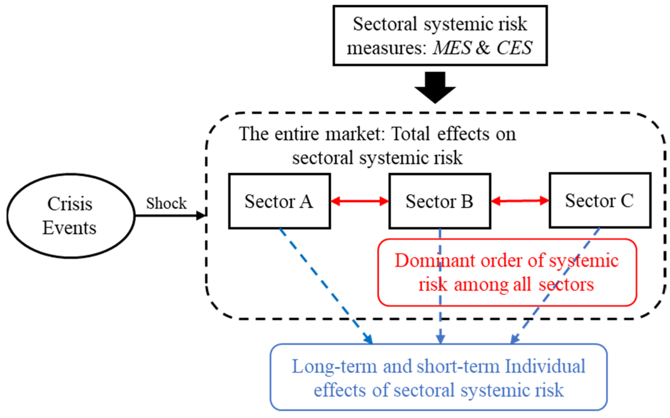
2.3. Testing the Total and Individual Effects of Crisis Events on Sectoral Systemic Risk

In this study, we employ the panel event study model, developed by Freyaldenhoven et al. (2019) [31], to capture the total impact of black swan events and financial turmoil on sectoral systemic risk in China’s financial market. By comparing the variation in estimators around the time baseline, this method can create a clear visual representation of the shock of the adoption of the event. A key assumption to be made is that, in order to ensure the consistent estimation of outcomes, the events are endogenously unrelated to the changes in the levels in posterior time. This model is extended from the standard two-way fixed effect model that includes all posterior periods and estimates the average treatment effect (Goodman-Bacon (2021) [33]). In contrast, the full setting of the event leads in the panel event study model takes into account the trends in the treated variables before the event occurs. In addition, the coefficients of the event lags show the dynamic nature of the impact of the events over time, implying that their influence is transitory or permanent. Consider a panel that covers sectors $i$ and time periods $t$, the panel event study model can be shown as follows:

$$y_{i,t}=\alpha +{\displaystyle \sum }_{j=2}^J{\beta }_j{\left(\mathrm{Lag} j\right)}_{i,t}+{\displaystyle \sum }_{k=2}^K{\gamma }_k{\left(\mathrm{Lead} k\right)}_{i,t}+X_{i,t}^{\prime }\Gamma +{\iota }_i+{\nu }_t+{\epsilon }_{i,t}$$

(15)

where $y_{i,t}$ denotes the independent variable, which is the systemic risk level of each sector, $X_{i,t}$ represents the control variables, ${\iota }_i$ and ${\nu }_t$are the sector and time fixed effects, and ${\epsilon }_{i,t}$ is the error term. We use $Even{t}_i$ to denote the time at which sector $i$ is influenced by the occurrence of the event; then, the variables of lead and lag in Equation (15) are defined as follows:

$${\left(\mathrm{Lag} J\right)}_{i,t}=1\left[t\le Even{t}_i-J\right],$$

(16)

$${\left(\mathrm{Lag} j\right)}_{i,t}=1\left[t=Even{t}_i-j\right] \mathrm{for} j\in \left\{1,\dots ,J\right\},$$

(17)

$${\left(\mathrm{Lead} k\right)}_{i,t}=1\left[t=Even{t}_i+k\right] \mathrm{for} k\in \left\{1,\dots ,K\right\},$$

(18)

$${\left(\mathrm{Lead} K\right)}_{i,t}=1\left[t\ge Even{t}_i+k\right].$$

(19)

Thus, lag and lead are dummy variables that denote the given situation of the periods around the events. The same as the standard in Raftopoulou and Giannakopoulos (2022) [45] and Clarke and Tapia-Schythe (2021) [46], we set the first lag as the baseline omitted case in our empirical estimation, where $j=1$. Following the framework of the panel event study model, we examine the total effects and dynamic tendencies of sectoral systemic risk in the entire market with the occurrence of three emergency shock events.

Furthermore, consistent with Bernal et al. (2014) [39] and Morelli and Vioto (2020) [38], we apply two nonparametric methods, the Wilcoxon signed rank sum test and the bootstrap Kolmogorov–Smirnov test, to investigate the changes in the individual effects of the systemic risk level and its dominant order of different sectors during the black swan events. The Wilcoxon test can consider the positive or negative differences in ranks and also the magnitude between a pair of samples that are independent of each other, but without the assumption of the symmetric normal distribution of them (Hollander et al. (2015) [47]). The null hypothesis is that the median difference in pairs is equal to zero. When two samples are from the same distribution, the results are not significant. As with Morelli and Vioto (2020) [38], who use this method for paired data to test whether the levels of the conditional Value-at-Risk of banks, insurance and brokerages, and real estate companies are higher due to the crisis events, we test whether or not the marginal and absolute contributions of the systemic risk of each sector in China’s financial market in the period after a shock event, such as the COVID-19 outbreak, are greater than those in the period before. Therefore, in this study, the Wilcoxon signed rank sum test is applied to the following hypotheses:

$$H_0:CE{S}_{t:t+h-1}^i \le CE{S}_{t-h-1:t-1}^i, H_1:CE{S}_{t:t+h-1}^i>CE{S}_{t-h-1:t-1}^i$$

(20)

$$H_0:ME{S}_{t:t+h-1}^i\le ME{S}_{t-h-1:t-1}^i, H_1:ME{S}_{t:t+h-1}^i>ME{S}_{t-h-1:t-1}^i$$

(21)

where $i$ denotes different sectors, $h$ is the time horizon before or after the occurrence of events at time $t$, and $CES/MES$ are the measures of the marginal expected shortfall and the component expected shortfall, as defined in Section 2.1. For each case, the rejection of the null hypothesis $H_0$ and the positive test result imply that the systemic risk level of this financial sector significantly increases during the crisis event, or that the rejection of the null hypothesis with a negative value means that the sectoral systemic risk significantly decreases after the crisis event; otherwise, the difference between these two periods is not significant.

In addition, we employ the bootstrap Kolmogorov–Smirnov (KS) test, as proposed by Abadie (2002) [48], to test the contribution of each sector to the systemic risk of the entire market and the dominant relationship among them. This resampling approach is better than the traditional KS test because it avoids the Durbin problem. The goal setting of the bootstrap KS test involves the cumulative distribution functions (CDF) rather than the means, which are more easily influenced by the extremums. In addition, the asymptotically distribution-free property of this nonparametric method means that it does not require any assumptions about the underlying distribution, which could minimize the risk of errors. For the dominance test, we test whether or not the systemic risk of sector $j$ contributes more than sector $i$, which can represent the dominant order among the financial sectors. The two-sample KS statistic is also defined as follows:

$$K{S}_{m_1{m}_2}=\sqrt{\frac{m_1{m}_2}{m_1+m_2}}\underset{x}{\sup }\left|S_{m_1}\left(x\right)-L_{m_2}\left(x\right)\right|$$

(22)

where $S_{m_1}\left(x\right)$ and $L_{m_2}\left(x\right)$ denote the CDFs of the CES or MES of the two different sectors $j$ and $i$. The null hypothesis is defined as follows:

$$H_0:CE{S}_{0.05}^j \le CE{S}_{0.05}^i, H_1:CE{S}_{0.05}^j>CE{S}_{0.05}^i$$

(23)

$$H_0:ME{S}_{0.05}^j \le ME{S}_{0.05}^i, H_1:ME{S}_{0.05}^j>ME{S}_{0.05}^i$$

(24)

The rejection of the null hypothesis implies that the contribution magnitude of the systemic risk of sector $j$ to the entire market is larger than that of sector $i$, which also shows that the dominant rank of the systemic risk of sector $j$ is higher than that of sector $i$. By conducting the bootstrap KS test above, we can identify not only the significance of the individual effect of systemic risk in one sector, but also the dominant order of the individual effect of systemic risk among different sectors. On the basis of that, this paper addresses a relationship network that exists between the individual effects of sectoral systemic risk in order to analyze the evolution of the connectedness of systemic risk dominance between sectors during financial crisis events.

2.4. Data and Variables

Following the estimation framework of CES and MES in Section 2.2, we collect data from the WIND database; this includes weekly returns expressed in the logarithmic scale of the stock indices, and the weekly capitalization sizes of the A-share financial sectors and the market. The market data used for the systemic risk measure calculation cover a total of 424 weeks that range from 1 January 2014, to 1 April 2022. Based on the criterion of the industrial classification of China’s financial market, these sectors cover all 11 of the WIND Class I industries, which contain Energy (EN), Materials (MA), Industrials (IN), Consumer Discretionary (CD), Consumer Staples (CS), Healthcare (HE), Financials (FE), Information Technology (IT), Telecom Service (TS), Utilities (UT), and Real Estate (RE). We choose the Shanghai Stock Exchange Composite Index as the representation of the entire financial market.

Table 1. Descriptive statistics of sectoral returns.

	Mean	Max.	Min.	Stand. Dev.	Skewness	Kurtosis	J.B. Test	L.B. Q-Test
Energy	0.028	6.219	−7.759	1.592	−0.687	6.774	285.101 ***	235.701 ***
Materials	0.103	5.434	−11.470	1.774	−1.134	8.397	605.620 ***	317.333 ***
Industrials	0.071	5.220	−11.135	1.714	−1.245	9.522	861.130 ***	363.099 ***
Consumer_ Discretionary	0.056	5.109	−9.316	1.640	−1.135	8.044	540.778 ***	415.668 ***
Consumer_ Staples	0.136	4.560	−8.704	1.579	−1.106	6.812	343.353 ***	165.745 ***
Healthcare	0.086	5.663	−7.218	1.653	−0.763	5.833	182.998 ***	340.142 ***
Financials	0.083	6.878	−5.882	1.461	0.094	5.785	137.714 ***	112.688 ***
Information_ Technology	0.095	7.668	−10.040	2.057	−0.807	6.715	289.910 ***	474.665 ***
Telecom_ Service	0.009	7.453	−9.661	1.933	−0.573	6.623	255.178 ***	258.119 ***
Utilities	0.064	5.127	−11.948	1.488	−1.576	14.531	252.480 ***	172.600 ***
Real Estate	0.065	5.916	−9.520	1.786	−0.660	6.208	212.681 ***	233.441 ***

Note: *** indicates significance at the level of 0.01. The number of observations is 4664. J.B. test denotes the Jarque–Bera statistic for the test of normality and L.B. Q-test denotes the Ljung–Box statistic for serial autocorrelation in the squared returns.

presents the descriptive statistics of all sectoral returns. The skewness statistic shows a longer left tail for most sectors except for Financials, which indicates that Financials experiences more frequent periods of negative returns than others. The results of the Jarque–Bera test and the Ljung–Box Q-test for all sectoral returns reject the null hypotheses of normal distribution and reveal no ARCH effects in the time series for most cases.

To examine the total effects of sectoral systemic risk in the market during the COVID-19 outbreak, we employ the panel event study method, which is based on the description in Section 2.3. For emergency crisis events, following Huang et al. (2022) [2], we choose three main representative black swan events in China’s financial market: the implementation of the deleveraging policy in China’s A-share market in 2015, the announcement the US placing additional trade tariffs on China’s goods in 2018 and the outbreak of COVID-19 in 2020. The first incident dated to when the China Securities Regulatory Commission (CSRC) was reported to be carrying out a strict investigation into over-the-counter illegal funding on the 12 June 2015 (See website: http://www.csrc.gov.cn/csrc/c100029/c1000237/content.shtml (accessed on 9 March 2023)), and the second dated to when the United States Trade Representative (USTR) released a list of products imported from China, worth USD 50 billion, that would be subject to additional tariffs on 15 June 2018 (See website: https://ustr.gov/about-us/policy-offices/press-office/press-releases/2018/june/ustr-issues-tariffs-chinese-products(accessed on 9 March 2023)) [8]. In addition, in line with Tan et al. (2022) [49], the date set in the model for the outbreak of COVID-19 was 20 January 2020, when Chinese social media widely reported this public health event and it was confirmed by the government authorities (See website: http://www.gov.cn/xinwen/2020-01/20/content_5471057.htm (accessed on 9 March 2023)).

Table 2. Descriptions of variables in the panel event study model.

Variables	Descriptions	Measurements
Dependent variable
CES0.05/MES0.05	The level of sectoral systemic risk	The approaches to Component Expected Shortfall and Marginal Expected Shortfall, which measure the magnitude of systemic risk, are shown in Section 2.1
Explanatory variables
Lead/Lag	Temporal dummy variables	The binary variables indicate the given states in the pre-event or post-event periods
Control variables
Returns	Sectoral profitability	Total average return of sectoral index within one week
Volatility	Sectoral volatility	The percent of rise or fall of sectoral index within one week
Size	Sectoral market size	The logarithm scale of the average amount of market capitalization of the sectoral index within one week
Liquidity	Sectoral liquidity	The liquidity level of a sector within one week, measured by ILLIQ (Amihud and Noh (2021) [53])

provides detailed descriptions and measurements of all variables. The main independent variables in the panel event study model are the two measures of systemic risk, the Marginal Expected Shortfall and the Component Expected Shortfall (CES and MES) of all 11 sectors in China’s financial market. Based on Tian et al. (2022) [50], the length of the time horizon of the event study is set to 20 periods of sample time (weeks), which allows us to identify the impact of the event’s shock both in the short and long term. As shown in the model setting of Section 2.3, the event horizon includes the dummy variables of lead and lag, which are equal to one. To ensure the robustness of the estimators of the event’s lag and lead, we choose some control variables to reflect the different factors affecting the sectoral systemic risk level, which contain the profitability, volatility, market size and liquidity of financial sectors (e.g., Bernal et at., (2014) [39]; Chen and Jin (2020) [51]; and Yang et al., (2020) [52]).

Table 3. Descriptive statistics of variables.

Variables	Observations	Mean	Std. Dev.	Min.	Max.
CES0.05	4521	0.194	0.197	0.003	2.097
MES0.05	4521	2.177	1.363	0.001	13.849
Returns	4521	0.077	1.717	−11.948	7.668
Volatility	4521	0.256	3.903	−24.051	19.311
Size	4521	3.564	0.490	2.009	4.291
Liquidity	4521	0.022	0.068	0.001	1.461

present the descriptive statistics of all variables.

3. Empirical Results and Analyses

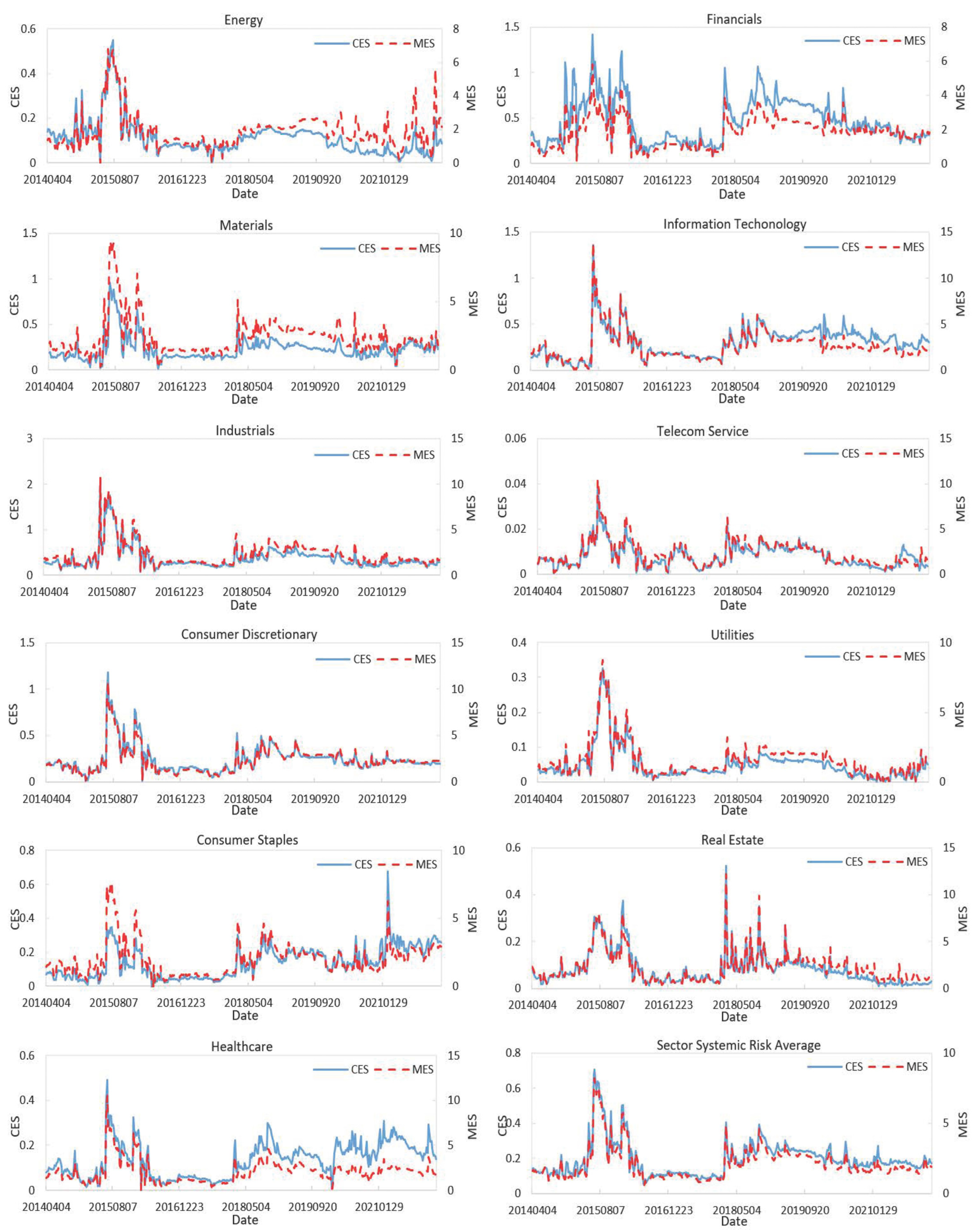
3.1. The Average Effects of Sectoral Systemic Risk during Crisis Periods

In accordance with the estimation process in Section 2.2, we calculate two types of sectoral system risk measures (CES and MES) to demonstrate the absolute and marginal contribution of systemic risk to the market, and each of them is based on the sectoral idiosyncratic risk level in a high or low degree, which is denoted by $Va{R}_{0.05}$ or $Va{R}_{0.5}$. Therefore, we obtain $CE{S}_{0.05}$, $CE{S}_{0.5}$, $ME{S}_{0.05}$, and $ME{S}_{0.5}$ for all 11 financial sectors corresponding to the two risk thresholds, the extreme case and the normal case. The total sample period is 411 weeks, which ranges from 31 March 2014 to 1 April 2022, and we draw three subsamples to represent the periods of financial turmoil in China’s A-share market to compare the average effects of sectoral systemic risk within these periods. The first is the period of the A-share market crash in 2015 (Period I) from 12 June 2015 to 5 February 2016 (34 weeks), the second is the period of Sino–US trade friction in 2018 (Period II) from 15 June 2018 to 28 December 2018 (47 weeks), and the third is the period of the first wave of the COVID-19 pandemic in 2020 (Period III) from 20 January 2020 to 24 April 2020 (12 weeks). Figure 2 illustrates the temporal change in the sectoral systemic risk measures, $CE{S}_{0.05}$ and $ME{S}_{0.05}$, of all 11 sectors in all sample periods. From the subplot of the average sectoral systemic risk in Figure 2, we notice that both CES and MES experience severe fluctuations in the three crisis periods above.

The two panels in

Table 4. CES_0.05 and MES_0.05 of China’s financial sectors in different sample periods.

Panel A: CES0.05
	All Period		Period I		Period II		Period III
	Mean	S.D.	Mean	S.D.	Mean	S.D.	Mean	S.D.
Energy	0.111	0.082	0.273	0.143	0.130	0.020	0.088	0.021
Materials	0.230	0.129	0.505	0.232 3	0.290	0.065	0.250	0.057
Industrials	0.382 2	0.264 1	0.986 1	0.415 1	0.430 2	0.122 2	0.386 3	0.077
Consumer_ Discretionary	0.239	0.147	0.569 3	0.229	0.311	0.102	0.251	0.045
Consumer_ Staples	0.139	0.091	0.204	0.088	0.171	0.063	0.156	0.034
Healthcare	0.134	0.078	0.228	0.086	0.167	0.062	0.151	0.083 3
Financials	0.464 1	0.245 2	0.794 2	0.253 2	0.651 1	0.195 1	0.539 1	0.098 1
Information_ Technology	0.299 3	0.165 3	0.566	0.229	0.370 3	0.119 3	0.402 2	0.088 2
Telecom_ Service	0.008	0.005	0.016	0.008	0.012	0.003	0.007	0.002
Utilities	0.051	0.049	0.174	0.082	0.058	0.017	0.049	0.008
Real Estate	0.081	0.068	0.218	0.068	0.129	0.081	0.077	0.023
Panel B: MES0.05
	All Period		Period I		Period II		Period III
	Mean	S.D.	Mean	S.D.	Mean	S.D.	Mean	S.D.
Energy	1.869	1.069	3.851	1.709	1.997	0.241	2.162	0.492
Materials	2.345	1.370	5.332 3	2.390 2	2.990	0.694	2.831 1	0.650 3
Industrials	2.287 2	1.435 3	5.391 2	2.215 3	2.678	0.785	2.515	0.480
Consumer_ Discretionary	2.315	1.369	5.134	2.152	2.936	1.057 3	2.806 2	0.500
Consumer_ Staples	1.957	1.268	4.297	1.933	2.638	0.970	1.863	0.428
Healthcare	2.028	1.266	4.661	1.861	2.514	0.944	1.919	1.054 1
Financials	1.841	0.876	3.002	0.984	2.496	0.645	2.147	0.381
Information_ Technology	2.608 1	1.601 1	5.941 1	2.424 1	3.485 1	1.176 2	2.616	0.546
Telecom_ Service	2.265 3	1.391	4.522	2.177	3.376 2	0.883	1.761	0.476
Utilities	1.564	1.319	4.611	2.086	1.897	0.535	1.805	0.297
Real Estate	2.179	1.592 2	5.113	1.732	3.311 3	2.042 1	2.539 3	0.754 2

Note: The upper corner marks of ¹, ², ³ denote the top three ranks of values in each column. Period I is the 34 weeks from 12 June 2015 to 5 February 2016, Period II is the 47 weeks from 15 June 2018 to 28 December 2018, and Period III is the 12 weeks from 20 January 2020 to 24 April 2020.

give the primary mean and standard deviation statistics of CES and MES in China’s financial sectors during different sample periods. It is obvious that all the values in Panel A and Panel B are larger than those matching those of the same sector in Appendix A 

Table A1. CES_0.5 and MES_0.5 of China’s financial sectors in different sample periods.

Panel A: CES0.05
	All Period		Period I		Period II		Period III
	Mean	S.D.	Mean	S.D.	Mean	S.D.	Mean	S.D.
Energy	0.045	0.032	0.111	0.046	0.043	0.005	0.039	0.010
Materials	0.091	0.048	0.194	0.082	0.083	0.020	0.108	0.027
Industrials	0.149 2	0.093 2	0.385 1	0.148 1	0.122 2	0.034 2	0.176 3	0.042 3
Consumer_ Discretionary	0.088	0.053	0.218 3	0.079	0.084	0.027	0.103	0.019
Consumer_ Staples	0.051	0.031	0.078	0.026	0.042	0.020	0.071	0.020
Healthcare	0.049	0.027	0.089	0.033	0.053	0.021	0.055	0.032
Financials	0.185 1	0.097 1	0.303 2	0.084 2	0.156 1	0.037 1	0.242 1	0.048 1
Information_ Technology	0.118 3	0.062 3	0.217	0.083 3	0.113 3	0.030 3	0.185 2	0.048 2
Telecom_ Service	0.003	0.002	0.007	0.003	0.003	0.001	0.005	0.001
Utilities	0.020	0.017	0.064	0.024	0.017	0.004	0.020	0.003
Real Estate	0.032	0.024	0.088	0.026	0.037	0.022	0.033	0.011
Panel B: MES0.05
	All Period		Period I		Period II		Period III
	Mean	S.D.	Mean	S.D.	Mean	S.D.	Mean	S.D.
Energy	0.748	0.402	1.586	0.572	0.666	0.055	0.951	0.247
Materials	0.926 2	0.507	2.056	0.871 2	0.860	0.216	1.220 1	0.305 3
Industrials	0.896 3	0.501	2.107 2	0.799 3	0.757	0.217	1.145 3	0.264
Consumer_ Discretionary	0.848	0.484	1.963	0.754	0.786	0.248	1.144	0.219
Consumer_ Staples	0.721	0.425	1.631	0.576	0.653	0.313	0.844	0.245
Healthcare	0.769	0.464	1.809	0.695	0.786	0.309 3	0.698	0.408 1
Financials	0.730	0.330	1.142	0.306	0.598	0.115	0.964	0.187
Information_ Technology	1.024 1	0.599 1	2.316 1	1.017 1	1.056 1	0.276	1.203 2	0.304
Telecom_ Service	0.888	0.528 3	1.842	0.690	0.954 3	0.347 2	1.128	0.281
Utilities	0.610	0.432	1.693	0.586	0.565	0.145	0.742	0.126
Real Estate	0.877	0.532 2	2.064 3	0.638	0.959 2	0.545 1	1.074	0.339 2

Note: The upper corner marks of ¹, ², ³ denote the top three ranks of values in each column. Period I is 34 weeks from 12 June 2015, to 5 February 2016, Period II is 47 weeks from 15 June 2018, to 28 December 2018, and Period III is 12 weeks from 20 January 2020, to 24 April 2020.

, indicating that the sectoral systemic risk of all sectors has a higher magnitude and volatility in the extreme risk status. Therefore, we use CES_0.05 and MES_0.05 as the main sectoral systemic risk measures. In the total sample period, the Financials, Industrials, and Information Technology sectors have the highest means and volatilities in terms of CES, which implies that these sectors have the contribute the most systemic risk to the market. We calculate the CES% of these three sectors to show the temporal change in their proportion of systemic risk among all sectors (see Appendix A Figure A1). In addition, the results of MES in all the sample periods show that, without considering the weight of the market size, the top three sectors with the highest marginal contribution of systemic risk are the Information Technology, Industrials, and Telecom Service sectors.

For the periods of the three financial market crises, we notice that the mean and volatility values of sectoral systemic risk in columns (3) to (8) are all higher than those in columns (1) and (2). By analyzing the results of CES_0.05 and MES_0.05 in Panel A and Panel B in Table 4, it is evident that financial turmoil and instability lead to the systemic risk of each factor presenting a stronger contribution in the mean level. During the A-share market crash period in 2015 (Period I), the Industrials and Financials sectors are the most important contributor, as well as during the trade friction crisis in 2018 (Period II); however, the Information Technology, Telecom Service, and Real Estate sectors present the strongest marginal systemic risk to the market. The outbreak of the COVID-19 pandemic in 2020 (Period III) also causes a market crisis, although the Financials, Information Technology, and Industrials sectors are still the top three sectors in the value of CES_0.05; indeed, the mean level of MES_0.05 of the Materials, Consumer Discretionary, and Real Estate sectors soar during this period. The economic lockdown and consumption crunch due to the COVID-19 pandemic have severe impacts on these sectors, and then enhance their marginal systemic risk contribution to the entire market. Moreover, we find that the volatilities of CES_0.05 and MES_0.05 in terms of the Healthcare sector increase remarkably, which could be regarded as an intuitive reaction of the financial market to this public health crisis.

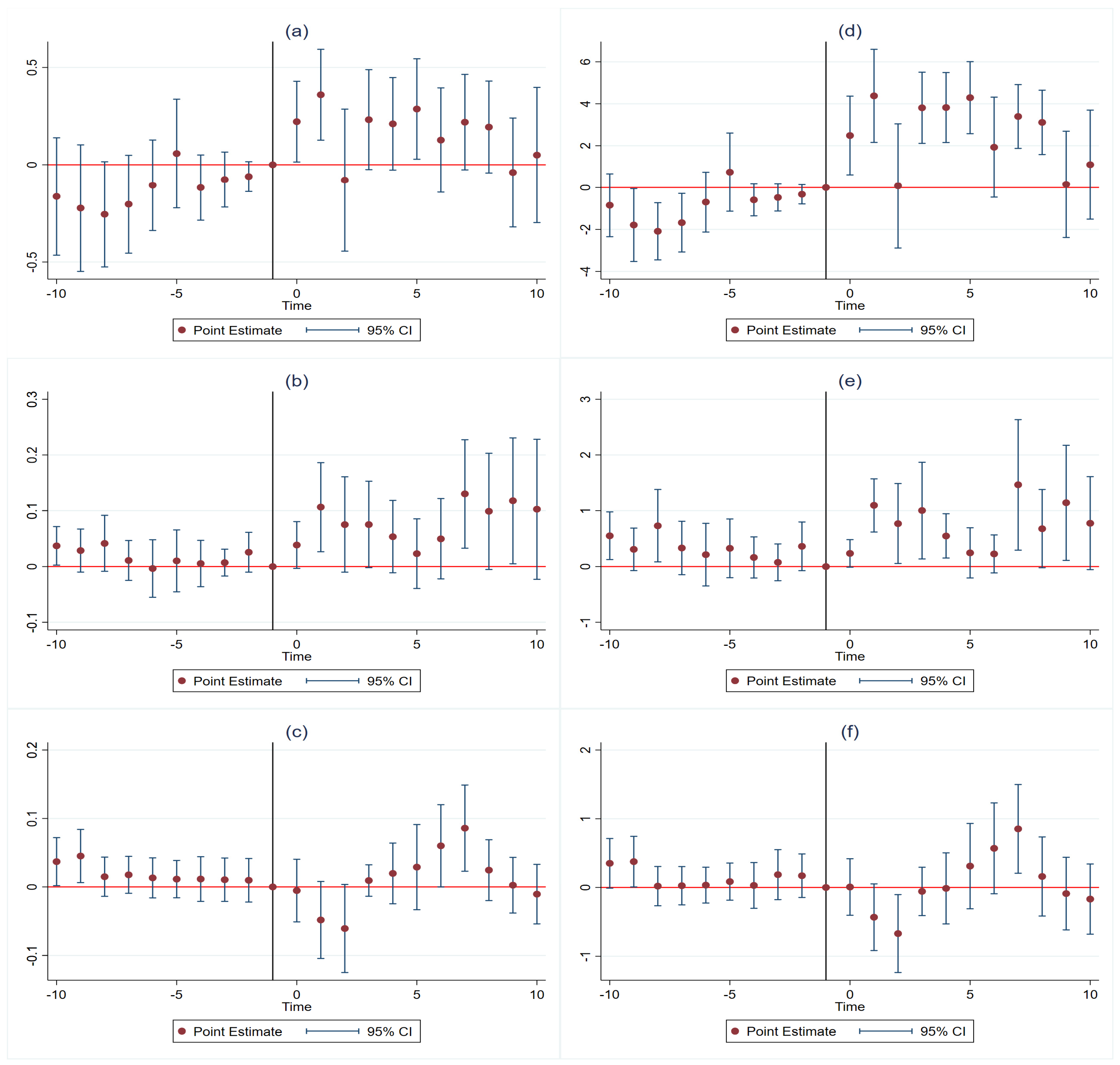
3.2. The Total Effects of Crisis Events on Sectoral Systemic Risk

In this section, following the research designs of Freyaldenhoven et al. (2019) [31] and Raftopoulou and Giannakopoulos (2022) [45], we adopt a panel event study model that is based on Equation (16) in order to examine the total effects of the occurrence of black swan events, such as the outbreak of COVID-19, in terms of sectoral systemic risk on the financial market. In addition, another two shock events are used to analyze the impacts of sectoral systemic risk on the entire market in different risk situations comparatively. As presented in Section 2.4, the key dates that we choose for the events are 20 January 2020, for the COVID-19 outbreak, 12 June 2015, for CSRC’s deleveraging policy implementation, and 15 June 2018, for the announcement of the US’s additional trade tariffs list, which correspond to the 300th week, the 64th week, and the 218th week in the total sample period, respectively. Consistent with Tian et al. (2022) [50], the event window is set as 20 periods (weeks), which is $\left[-10, 10\right]$ around the key dates of the events. The two-way fixed effects are considered in the model setting [54]. We also choose sectoral profitability, sectoral volatility, sectoral market size and sectoral liquidity as control variables to check the robustness of the regressions.

Table 5. The estimation results of the panel event study models with three different shock events.

Panel A: Sectoral Systemic Risk CES0.05
	Event I: CSRC’s Deleveraging Policy in 12 June 2015			Event II: US’s Additional Trade Tariffs in 15 June 2018			Event III: COVID-19 Outbreak in 20 January 2020
Constant	2.915 ** (0.015)	2.088 *** (0.003)	3.107 (0.302)	2.118 *** (0.002)	1.983 *** (0.000)	1.177 (0.555)	0.225 (0.554)	0.228 *** (0.000)	0.193 (0.348)
Leads /Lags		Yes	Yes		Yes	Yes		Yes	Yes
Returns	−0.412 *** (0.002)		−0.463 *** (0.001)	−0.192 * (0.085)		−0.258 * (0.089)	−0.237 ** (0.010)		−0.249 *** (0.003)
Volatility	0.176 *** (0.002)		0.201 *** (0.000)	0.091 * (0.091)		0.116 * (0.095)	0.101 ** (0.011)		0.108 *** (0.003)
Size	−0.712 (0.136)		−0.818 (0.336)	−1.378 (0.427)		−0.273 (0.622)	−0.004 (0.971)		0.326 (0.248)
Liquidity	−1.505 *** (0.002)		−2.462 *** (0.002)	−0.047 (0.348)		−0.016 (0.468)	−0.038 * (0.051)		−0.071 * (0.082)
Sector-fixed	Control	Control	Control	Control	Control	Control	Control	Control	Control
Time-fixed	Control	Control	Control	Control	Control	Control	Control	Control	Control
L-likelihood	−2.503	65.813	82.031	341.149	368.109	372.024	381.378	427.016	434.916
AIC	13.006	−111.626	−144.063	−674.298	−716.219	−724.049	−754.757	−834.033	−849.831
BIC	26.775	−77.201	−109.639	−660.528	−681.795	−689.624	−740.987	−799.609	−815.407
R-squared	0.177	0.545	0.604	0.361	0.493	0.511	0.156	0.364	0.406
Observations	231	231	231	231	231	231	231	231	231
Panel B: Sectoral Systemic Risk MES0.05
	Event I: CSRC’s Deleveraging Policy in 12 June 2015			Event II: US’s Additional Trade Tariffs 15 June 2018			Event III: COVID-19 Outbreak in 20 January 2020
Constant	3.102 *** (0.008)	2.420 *** (0.000)	1.528 (0.337)	6.002 *** (0.000)	2.257 *** (0.000)	5.145 (0.105)	1.938 ** (0.025)	2.535 *** (0.000)	1.011 (0.469)
Leads /Lags		Yes	Yes		Yes	Yes		Yes	Yes
Returns	−4.146 *** (0.000)		−4.267 *** (0.001)	−2.863 ** (0.024)		−3.764 *** (0.000)	−3.074 *** (0.009)		−3.567 ** (0.013)
Volatility	1.770 *** (0.000)		1.825 *** (0.001)	1.322 ** (0.019)		1.675 *** (0.000)	1.323 *** (0.009)		1.566 ** (0.012)
Size	−7.528 (0.317)		−3.624 (0.415)	−1.618 (0.517)		−1.373 (0.489)	−4.784 (0.441)		−2.134 (0.581)
Liquidity	−3.361 * (0.068)		−1.158 *** (0.009)	−0.982 (0.558)		−1.130 (0.694)	−2.701 *** (0.000)		−2.210 *** (0.009)
Sector-fixed	Control	Control	Control	Control	Control	Control	Control	Control	Control
Time-fixed	Control	Control	Control	Control	Control	Control	Control	Control	Control
L-likelihood	−526.357	−383.974	−362.676	−207.843	−202.217	−185.305	−150.801	−111.089	−98.567
AIC	1060.714	787.949	745.352	423.687	424.433	390.610	309.602	242.178	217.135
BIC	1074.484	822.373	779.776	437.457	458.857	425.035	323.372	276.602	251.560
R-squared	0.231	0.775	0.813	0.401	0.429	0.506	0.131	0.383	0.446
Observations	231	231	231	231	231	231	231	231	231

Note: In the parentheses are the p value and *, ** and ***, which indicate significance at the 10%, 5% and 1% levels, respectively.

shows the main estimation results of the panel event study models using three different black swan shock events.

The results in Table 5 contain the estimation outcomes of basic panel two-way fixed effect models, and the panel event study models with or without control variables. The main independent variable is the sectoral systemic risk measure CES_0.05 in Panel A and MES_0.05 in Panel B. By comparing the R-square, loglikelihood, AIC and BIC values of each model, we find that the panel event study model with control variables is superior to the other models during model selection, which indicates that our model setting is robust. With respect to control variables, the sectoral profitability is significantly negative in all models, both in Panel A and Panel B. In addition, the sectoral volatility variable that is the percent of rise or fall of the sectoral index is significantly positively correlated with the level of CES_0.5 and MES_0.5. In line with Drakos and Kouretas (2015) [55] and Chen and Jin (2020) [51], these two results indicate that high returns will smooth the sectoral systemic risk level, whereas high volatility will enhance it during the crisis. In addition, despite there being a correlation between institution-level systemic risk and its capitalization (Laeven et al., (2016) [56]), we find no significant evidence that the market size of a sector is related to the level of its CES or MES in a time of distress. This is might due to the fact that the sectoral size is not a significant factor in the marginal contribution of sectoral systemic risk, as shown in Section 2.2. As for CES, on the one hand, the non-significant relationship in the pre-event period may cause the same result between size and CES in the total event time horizon, which covers up the results of significance in the post-event period. On the other hand, the sector-level concentration would also lower the size effects of sectoral systemic risk exposure [57]. In addition, different sectors perform differently during different crisis events, so may not have the same impact on the sectoral systemic risk themselves [58]. This heterogeneity in terms of sector size across all sectors, caused by the connectedness and spillover of fluctuations in the price of assets among them, is another explanation [59,60]. Finally, we notice that a liquidity risk in the market remarkably amplifies the sectoral systemic risk at the time of the A-share market crash in 2015 and the COVID-19 outbreak in 2020. This type of mutual spiral relationship between a market liquidity crunch and systemic risk, especially during a sudden market crisis, is consistent with Louhichi et al. (2022) [61].

Figure 3 explicitly presents the estimation results of the lead/lag variables of the panel event study models in Table 5, which illustrate the dynamic total effects of sectoral systemic risk on the entire market during different black swan events. All the estimation outcomes of the lead and lag variables in the event window are also given in Appendix A 

Table A2. The estimation results of dynamic total effects of sectoral systemic risk in different events.

	Sectoral Systemic Risk CES0.05			Sectoral Systemic Risk MES0.05
	Event I	Event II	Event III	Event I	Event II	Event III
Lead10	−0.163 (0.257)	0.037 ** (0.038)	0.037 ** (0.041)	−0.845 (0.238)	0.552 ** (0.016)	0.351 * (0.056)
Lead9	−0.223 (0.158)	0.028 (0.129)	0.045 ** (0.027)	−1.790 ** (0.044)	0.309 (0.101)	0.375 ** (0.046)
Lead8	−0.254 * (0.062)	0.042 * (0.094)	0.015 (0.273)	−2.088 *** (0.007)	0.732 ** (0.030)	0.019 (0.883)
Lead7	−0.203 (0.103)	0.011 (0.509)	0.017 (0.176)	−1.678 ** (0.023)	0.334 (0.152)	0.025 (0.844)
Lead6	−0.105 (0.336)	−0.003 (0.884)	0.013 (0.338)	−0.695 (0.304)	0.214 (0.416)	0.034 (0.777)
Lead5	0.057 (0.655)	0.010 (0.690)	0.011 (0.374)	0.737 (0.400)	0.328 (0.196)	0.085 (0.500)
Lead4	−0.117 (0.150)	0.005 (0.776)	0.012 (0.450)	−0.591 (0.115)	0.164 (0.346)	0.029 (0.847)
Lead3	−0.076 (0.258)	0.007 (0.526)	0.010 (0.476)	−0.477 (0.131)	0.076 (0.619)	0.186 (0.280)
Lead2	−0.061 (0.108)	0.025 (0.140)	0.009 (0.511)	−0.323 (0.149)	0.363 * (0.094)	0.171 (0.258)
Lag0	0.221 ** (0.039)	0.038 * (0.067)	−0.005 (0.800)	2.486 ** (0.015)	0.236 * (0.059)	0.007 (0.971)
Lag1	0.359 *** (0.006)	0.106 ** (0.014)	−0.048 * (0.085)	4.378 *** (0.001)	1.095 *** (0.000)	−0.433 * (0.075)
Lag2	−0.079 (0.639)	0.075 * (0.078)	−0.060 * (0.062)	0.079 (0.954)	0.771 ** (0.037)	−0.670 ** (0.025)
Lag3	0.232 * (0.072)	0.075 * (0.055)	0.009 (0.388)	3.809 *** (0.001)	1.002 ** (0.027)	−0.057 (0.723)
Lag4	0.210 * (0.077)	0.054 * (0.095)	0.019 (0.345)	3.822 *** (0.000)	0.549 ** (0.011)	−0.013 (0.955)
Lag5	0.287 ** (0.033)	0.023 (0.427)	0.029 (0.324)	4.292 *** (0.000)	0.246 (0.251)	0.311 (0.291)
Lag6	0.127 (0.316)	0.049 (0.154)	0.060 * (0.050)	1.929 (0.102)	0.227 (0.169)	0.569 * (0.084)
Lag7	0.219 * (0.075)	0.130 ** (0.014)	0.086 ** (0.013)	3.395 *** (0.001)	1.464 ** (0.019)	0.852 ** (0.015)
Lag8	0.194 * (0.097)	0.098 * (0.060)	0.024 (0.247)	3.113 *** (0.001)	0.679 * (0.056)	0.159 (0.550)
Lag9	−0.039 (0.758)	0.117 ** (0.042)	0.003 (0.893)	0.153 (0.896)	1.142 ** (0.033)	−0.089 (0.714)
Lag10	0.049 (0.756)	0.103 * (0.099)	−0.011 (0.601)	1.094 (0.371)	0.778 * (0.064)	−0.169 (0.478)

Note: In the parentheses are the p value and *, ** and *** indicate significance at the 10%, 5% and 1% levels, respectively.

. As shown in Figure 3, most of the coefficients of the lead variables before the shock event are not significantly different from zero at the 5% significance level, and show no clear trends in terms of the changing mode; this indicates that sectoral systemic risk has no significant influence on the entire market in the pre-event period. This result verifies the exogenous requirement for events that is the occurrence of the market crisis shock does not affect the total effect of sectoral systemic risk in advance. During the post-event period, it is obvious that there exists a significant enhancement in the total effect of sectoral systemic risk both in the plots of CES and MES. After the CSRC’s investigation into over-the-counter illegal funding was widely reported, the total effect immediately surged at the time of the event’s occurrence and the time of lag1, then increased again in the periods from lag3 to lag5 (see Figure 3a,d). Similarly, the US’s announcement of additional trade tariffs on goods from China caused a rise in the total effect of sectoral systemic risk at once, and a second wave of increase occurred after the time of lag 7 (see Figure 3b,e).

These results imply that both two events cause sustained shocks to the overall systemic risk of the entire market from the aspect of all sectors. In addition, we find that the effect of this kind of event on the marginal expected shortfall is larger than the component expected shortfall, which shows that the measure of MES has a sharper reaction to the sudden market crisis. Different from the influence patterns of events I and II, the sectoral systemic risk has a hysteresis effect of the market after the COVID-19 outbreak. As we can see in Figure 3c,f, the sectoral systemic risk slightly decreases at the time of lag 1 and lag 2, and abruptly increases from lag 3 to lag 7 after the COVID-19 pandemic is confirmed. This result, indicating that the sectoral systemic risk does not have a horizontal effect but instead a trend effect around the date of the COVID-19 pandemic, is consistent with Ouyang et al. (2022) [33]. The reasons for this are twofold; the first reason is that the sectoral heterogeneity of the COVID-19 outbreak has various impacts on different sectors (He et al. (2020) [29]), and the second one is that there exist dominant position transitions of sectoral systemic risk among sectors during the financial crisis (Zhang et al. (2020) [62]). From the long-term perspective, the persistence of the pandemic and the pessimistic outlook on economic growth eventually caused a positive shock to the sectoral systemic risk, the same as the results seen in regards to event I and event II. Therefore, it is necessary to analyze the individual effect of sectoral systemic risk and its dominant order among sectors during periods of the financial crisis.

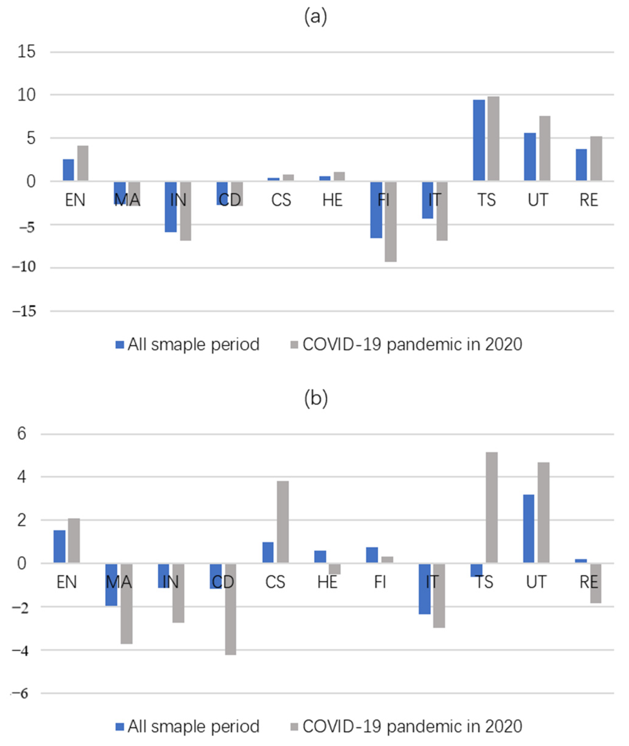
3.3. The Individual Effects of Crisis Events on Sectoral Systemic Risk

Table 6. The Wilcoxon signed rank sum tests of sectoral systemic risk during the three shock events.

${\mathit{H}}_0: \mathit{C}\mathit{E}\mathit{S}/\mathit{M}\mathit{E}{\mathit{S}}_{0.05, \mathit{t}:\mathit{t}+\mathit{h}-1}^{\mathit{i}} \le \mathit{C}\mathit{E}\mathit{S}/\mathit{M}\mathit{E}{\mathit{S}}_{0.05, \mathit{t}-\mathit{h}-1:\mathit{t}-1}^{\mathit{i}}$
Panel A: CES0.05
	Event I: CSRC’s Deleveraging Policy in 12 June 2015		Event II: US’s Additional Trade Tariffs in 15 June 2018		Event III: COVID-19 Outbreak in 20 January 2020
	Short Term	Long Term	Short Term	Long Term	Short Term	Long Term
Energy	−0.168 *** (0.002)	−0.219 *** (0.000)	−0.018 *** (0.004)	−0.023 *** (0.000)	−0.014 ** (0.041)	−0.009 * (0.086)
Materials	−0.555 *** (0.002)	−0.589 *** (0.000)	−0.042 ** (0.041)	−0.033 * (0.054)	−0.032 (0.484)	−0.048 * (0.076)
Industrials	−0.678 * (0.064)	−0.859 *** (0.003)	−0.099 ** (0.026)	−0.107 *** (0.002)	0.021 (0.588)	0.004 (0.850)
Consumer_ Discretionary	−0.698 *** (0.002)	−0.657 *** (0.000)	−0.134 *** (0.002)	−0.152 *** (0.000)	0.029 (0.132)	0.006 (0.191)
Consumer_ Staples	−0.251 *** (0.002)	−0.249 *** (0.000)	−0.048 * (0.065)	−0.089 *** (0.001)	−0.053 ** (0.015)	−0.043 ** (0.031)
Healthcare	−0.269 *** (0.002)	−0.254 *** (0.000)	−0.054 *** (0.009)	−0.077 *** (0.000)	−0.002 (0.394)	−0.048 ** (0.045)
Financials	−0.275 ** (0.026)	−0.283 *** (0.009)	−0.123 *** (0.002)	−0.147 *** (0.001)	0.049 (0.179)	0.033 (0.162)
Information_ Technology	−0.868 *** (0.002)	−0.744 *** (0.000)	−0.184 *** (0.004)	−0.161 *** (0.001)	0.060 (0.394)	0.047 * (0.075)
Telecom_ Service	−0.011 *** (0.002)	−0.009 *** (0.001)	−0.001 (0.179)	0.001 (0.623)	0.003 * (0.065)	0.003 *** (0.005)
Utilities	−0.148 *** (0.002)	−0.177 *** (0.000)	−0.020 *** (0.004)	−0.009 (0.104)	0.010 * (0.065)	0.009 *** (0.009)
Real Estate	−0.129 *** (0.002)	−0.152 *** (0.000)	−0.030 (0.699)	−0.037 (0.212)	0.007 (0.394)	0.004 (0.273)
Panel B: MES0.05
	Event I: CSRC’s Deleveraging Policy in 12 June 2015		Event II: US’s Additional Trade Tariffs in 15 June 2018		Event III: COVID-19 Outbreak in 20 January 2020
	Short Term	Long Term	Short Term	Long Term	Short Term	Long Term
Energy	−1.899 *** (0.002)	−2.818 *** (0.000)	−0.286 *** (0.004)	−0.292 *** (0.000)	−0.520 *** (0.004)	−0.469 ** (0.014)
Materials	−5.839 *** (0.002)	−6.151 *** (0.000)	−0.499 ** (0.041)	−0.399 ** (0.045)	−0.371 (0.588)	−0.530 * (0.074)
Industrials	−3.948 *** (0.065)	−4.759 *** (0.003)	−0.658 ** (0.026)	−0.726 *** (0.002)	0.234 (0.588)	−0.131 * (0.077)
Consumer_ Discretionary	−6.481 *** (0.002)	−5.998 *** (0.000)	−1.222 *** (0.002)	−1.463 *** (0.000)	0.249 (0.309)	−0.302 * (0.089)
Consumer_ Staples	−5.393 *** (0.002)	−5.265 *** (0.000)	−0.625 * (0.093)	−1.242 *** (0.002)	−0.660 ** (0.015)	−0.530 ** (0.011)
Healthcare	−5.798 *** (0.002)	−5.377 *** (0.000)	−0.709 *** (0.009)	−1.087 *** (0.000)	0.094 (0.588)	−0.477 * (0.076)
Financials	−0.877 * (0.079)	−0.882 ** (0.021)	−0.467 *** (0.002)	−0.536 *** (0.001)	0.042 (0.692)	−0.032 (0.850)
Information_ Technology	−9.193 *** (0.002)	−7.921 *** (0.000)	−1.651 *** (0.004)	−1.484 *** (0.001)	0.763 (0.179)	0.682 *** (0.009)
Telecom_ Service	−3.844 *** (0.002)	−3.028 *** (0.000)	−0.435 * (0.065)	−0.203 (0.521)	0.957 * (0.065)	0.887 *** (0.002)
Utilities	−3.627 *** (0.002)	−4.302 *** (0.000)	−0.665 *** (0.004)	−0.275 (0.307)	0.228 (0.179)	0.176 ** (0.037)
Real Estate	−3.478 *** (0.002)	−3.755 *** (0.000)	−0.924 (0.485)	−1.168 (0.121)	0.034 (0.394)	−0.085 * (0.077)

Note: Table shows the results of the Wilcoxon signed rank sum tests, which determines whether or not the level of systemic risk h-weeks after a shock event, or a period of financial crisis, is greater than the same h-weeks before. The hypothesis tested is $H_0:CES/ME{S}_{0.05, t:t+h-1}^i \le CES/ME{S}_{0.05, t-h-1:t-1}^i$, with $h=6$weeks of short term and $h=10$weeks of long term. In the parentheses are the p value and *, ** and ***, which indicate significance at the 10%, 5% and 1% levels, respectively.

presents the results of the Wilcoxon signed rank sum tests of sectoral systemic risk during the three shock events, which are the CSRC’s deleveraging policy implementation on 12 June 2015, the Sino–US trade friction engagement on 15 June 2018, and the COVID-19 outbreak on 20 January 2020. We employ this nonparametric test to detect whether or not the systemic risk level of each sector significantly changes after the occurrence of shock events. The event windows $\left[-6, 6\right]$ and $\left[-10, 10\right]$ are used to cover the sample periods around the date of events, which could help us to capture the individual effects of the absolute contribution and marginal contribution of the systemic risk of all 11 sectors in China’s financial market that are affected by market crisis events. This setting of two event windows is also considered a variation in CES and MES in the short term and long term, respectively [63]. According to Section 2.3, the null hypothesis of the test is $H_0:CES/ME{S}_{0.05, t:t+h-1}^i \le CES/ME{S}_{0.05, t-h-1:t-1}^i$, where $h$ is the breadth of the event window. In addition, due to the properties of Wilcoxon signed rank sum tests, the size and sign of the coefficients in Table 6 indicate the differences in the means between the samples in the pre-event periods and the post-event periods, which illustrate the changing trends in sectoral systemic risk around every black swan event.

For the results of sectoral systemic risk in Table 6, the negative/positive value of the outcomes shows that the level of sectoral systemic risk in post-event periods is larger/lower than that in pre-event periods. In two Panels A and B, the null hypothesis is rejected at a 5% significance level in most of the cases in columns (1) and (2), which indicates that the level of systemic risk in all sectors, regardless of whether it is in the short term or long term, is significantly influenced by the shock of the A-share market deleveraging policy in 2015. This finding shows that this event causes a massive market panic and becomes the source of the A-share market crash in that year. In particular, both in the short term and long term after the event, the Information Technology, Consumer Discretionary, and Industrials sectors are the most affected sectors in terms of the level of the absolute contribution of systemic risk, and Information Technology, Consumer Discretionary, and Materials are the most affected sectors in the level of the marginal contribution of systemic risk. By comparing the values in columns (1) and (2), we notice that the Energy, Materials, Industrials, Financials, Utilities, and Real Estate sectors are more profoundly influenced by the policy shock, while the effects on other sectors decline over time. As for the individual effects of the announcement of the US’s additional trade tariffs in 2018, it could be found that most of the sectors are impacted both in the short term and long term, except for Telecom Service, Utilities, and Real Estate. The change level of CES and MES in the Information Technology, Consumer Discretionary, Healthcare and Financials sectors are the highest, which shows that the contributions of systemic risk from these sectors are significantly amplified by the trade friction event. Moreover, there is also a long-term increase in the systemic risk level in the sectors of Energy, Industrials, Consumer Discretionary, Consumer Staples, Healthcare, and Financials. Corresponding to the results in Section 3.2, these two black swan events above have an industry-wide impact effect on China’s financial system, which highly strengthens the intensity of systemic risk contributed by most sectors to the entire market.

Contrarily, the outbreak of COVID-19 does not trigger a surge in systemic risk in all sectors. As shown in columns (5) and (6), the first batch of sectors shocked by the COVID-19 pandemic, both in the short and long term, are Energy and Consumer Staples. The former includes the coal, gas, oil mining, extraction, and electricity service industries, and the latter contains food and alcoholic drinks companies, retailers, and supermarkets, which are heavily influenced in the short term due to the transportation lockdown and the shrink in demand caused by virus outbreak (He et al. (2020) [29]). The panic and uncertainty of market investors about these sectors form low expectations, which further enhance their systemic risk level. It is noticeable that the level of the marginal expected shortfall in the Materials, Industrials, and Real Estate sectors also rises in the long term after COVID-19, which might be due to pessimistic judgments in terms of economic growth and low levels of capacity, due to shortages of labor (International Labor Organization (2021) [64]). This public health crisis leads to surges in turnover intention and a stronger desire for job security among employees (Mahmoud et al. (2021) [65]; Deng et al. (2022) [66]). Although many manufacturers transformed to produce medical equipment to avoid losses, there was a decrease in demand for the manufacture of vehicles and home appliances on account of the economic growth slowdown, and there was serious recession in seen in the tourism and hotel industry (Wu et al. (2021) [67]); these together led to a significantly positive reaction in the level of systemic risk in the Consumer Discretionary sector. Undoubtedly, the magnitude of CES and MES in Healthcare appears to have experienced the greatest increase among all sectors in the long term due to the pressure of the wide spread of COVID-19. However, the values of the Wilcoxon signed rank sum tests in the sectors of Information Technology, Telecom Service, and Utilities are significantly positive, which indicates that the level of systemic risk in these sectors is lower than those before the crisis. As argued by Liu et al. (2020) [68], the pandemic boosted the popularity of working, schooling, and entertaining at home, thus lifting demand in the Software and Telecom Service sectors and provoking their development. Better expectations and investment prospects lead to higher returns in the stock market, reducing the contribution of systemic risk from these sectors. In addition, we find that the systemic risk measures of the Financials sector are not impacted by this public health crisis, which implies that they are still at the same level during both the pre-event and post-event periods.

Additionally, it is noticed that the three main black swan events show different results for different sectors both in the short and long term in Table 6. The reason for this typical agglomeration of systemic risk in various sectors is mainly because of some of the characteristics of crisis events, such as the different sources of risk, the different degrees of risk, and the different affected industries. Basically, the extreme changes in the sectoral systemic risk level in the short term could be attributed to the high market volatility and financial environment instability [69]. However, the economic growth uncertainty and pessimistic expectation caused by these crisis events are regarded as the most influential factors in terms of causing long-lasting impacts on systemic risk in some sectors [70]. In addition, those sectors that show the amplifying shock effect of systemic risk level from the short term to long term are the most important risk contributors to the entire market. For instance, first, although the deleveraging policy in 2015 (Event I) caused an immediate all-sector surge in systemic risk, sectors such as Energy, Industrials, Utilities, and Real Estate showed a remarkably exacerbated effect in the long term (increase of more than 20%). As mentioned by Shen et al. (2021) [71], these sectors are generally basic industries, accounting for a great part of the economic structure in China and having strong associations with the other sectors. Therefore, they suffered the most sustained shock and became the largest systemic risk contributor during the A-share market crash in 2015. Second, the Sino–US trade friction in 2018 had a more direct impact on the sectors that export products that appeared on the US tariff list, such as the Information Technology, Consumer Discretionary, and Industrials sectors; this was then transmitted to other sectors such as Financials and Energy, which are connected to the target sectors [72]. Unlike Event I, we can see that the announcement of additional trade tariffs by the USTR (Event II) heavily shocked the related sectors, rather than all the other sectors, in the level of systemic risk. However, the economic uncertainty caused by trade friction eventually lead to the increase in CES and MES of most sectors in the long term. At last, the outbreak of the COVID-19 pandemic in 2020 (Event III) unquestionably influenced the systemic risk magnitude of Healthcare on a large scale. Due to the epidemic prevention policy, the lockdown of production and the cutoff of logistics and transportation also caused an increase in the negative effect of systemic risk in Consumer Staples, Materials, and Energy [73]. The aggregate impact of the COVID-19 pandemic on sectoral systemic risk is weaker than the other two crisis events above. Specially, we find that there exists a hedging risk effect in some sectors, such as Information Technology, Telecom Service, and Utilities, in which the systemic risk level decreases. Overall, by comparing the results for different sectors both in the short and long term during three crisis events, we can draw the conclusion that the intersectoral shocks of systemic risk, ignited by crisis events, mainly depend on the crises’ characteristics, which are different in terms of their source and degree.

3.4. The Dominant Order of Sectoral Systemic Risk during the COVID-19 Crisis

By referring to Mensi et al. (2017) [74] and Ji et al. (2018) [75], we employ the bootstrap Kolmogorov–Smirnov (KS) test to examine the dominant order of systemic risk among different sectors before and after emergency crisis events by using the COVID-19 outbreak as an example. As shown in Section 2.3, the bootstrap KS test is used to identify the differences between the cumulative distribution functions of CES or MES of various sectors, which illustrate the dominant order of the level of systemic risk among them. This nonparametric method can reveal the significant relationship, in terms of systemic risk measures, between two different sectors in relation to the sample’s numeric distribution during different time periods. By comparing the sequences constructed from the samples during the periods of crisis and no crisis, we can clearly understand the rank of the contribution magnitude of systemic risk and locate the position of each sector in this dominant relationship. In addition, we are able to capture the impacts of financial crisis on sectoral systemic risk, like that of Luo et al. (2021) [76], and the changes in each sector on the dominant order.

Table 7. Dominance test of CES of all sectors during all sample periods.

All Sample Periods (${\mathit{H}}_0: \mathit{C}\mathit{E}{\mathit{S}}_{0.05}^{\mathit{j}} \le \mathit{C}\mathit{E}{\mathit{S}}_{0.05}^{\mathit{i}}$)
	EN	MA	IN	CD	CS	HE	FI	IT	TS	UT	RE
EN		0.642 *** (0.000)	0.886 *** (0.000)	0.630 *** (0.000)	0.304 *** (0.000)	0.316 *** (0.000)	0.849 *** (0.000)	0.667 *** (0.000)	0.002 (0.997)	0.000 (1.000)	0.010 (0.961)
MA	0.000 (1.000)		0.411 *** (0.000)	0.095 ** (0.023)	0.000 (1.000)	0.000 (1.000)	0.521 *** (0.000)	0.370 *** (0.000)	0.000 (1.000)	0.000 (1.000)	0.000 (1.000)
IN	0.000 (1.000)	0.000 (1.000)		0.000 (1.000)	0.000 (1.000)	0.000 (1.000)	0.246 *** (0.000)	0.061 (0.213)	0.000 (1.000)	0.000 (1.000)	0.000 (1.000)
CD	0.000 (1.000)	0.071 (0.125)	0.394 *** (0.000)		0.000 (1.000)	0.000 (1.000)	0.506 *** (0.000)	0.341 *** (0.000)	0.000 (1.000)	0.000 (1.000)	0.000 (1.000)
CS	0.066 (0.164)	0.436 *** (0.000)	0.640 *** (0.000)	0.377 *** (0.000)		0.061 (0.213)	0.655 *** (0.000)	0.499 *** (0.000)	0.005 (0.990)	0.002 (0.997)	0.005 (0.990)
HE	0.046 (0.409)	0.384 *** (0.000)	0.710 *** (0.000)	0.397 *** (0.000)	0.107 *** (0.008)		0.720 *** (0.000)	0.543 *** (0.000)	0.005 (0.990)	0.002 (0.997)	0.005 (0.990)
FI	0.000 (1.000)	0.000 (1.000)	0.044 (0.448)	0.000 (1.000)	0.000 (1.000)	0.000 (1.000)		0.000 (1.000)	0.000 (1.000)	0.000 (1.000)	0.000 (1.000)
IT	0.002 (0.997)	0.046 (0.409)	0.260 *** (0.000)	0.029 (0.700)	0.002 (0.997)	0.005 (0.990)	0.326 *** (0.000)		0.002 (0.997)	0.002 (0.997)	0.005 (0.990)
TS	0.944 *** (0.000)	0.985 *** (0.000)	1.000 *** (0.000)	0.988 *** (0.000)	0.949 *** (0.000)	0.949 *** (0.000)	0.998 *** (0.000)	0.968 *** (0.000)		0.815 *** (0.000)	0.886 *** (0.000)
UT	0.545 *** (0.000)	0.869 *** (0.000)	0.949 *** (0.000)	0.847 *** (0.000)	0.543 *** (0.000)	0.572 *** (0.000)	0.929 *** (0.000)	0.835 *** (0.000)	0.019 (0.853)		0.314 *** (0.000)
RE	0.265 *** (0.000)	0.759 *** (0.000)	0.891 *** (0.000)	0.696 *** (0.000)	0.350 *** (0.000)	0.384 *** (0.000)	0.854 *** (0.000)	0.723 *** (0.000)	0.002 (0.997)	0.000 (1.000)

Note: The Table shows the results of the dominance test based on the two-sample Kolmogorov–Smirnov test. The null hypothesis is $H_0:CE{S}_{0.05}^j \le CE{S}_{0.05}^i$, which denotes that the systemic risk level related to the sector j (columns) is less risky (or equally) than the systemic risk level related to the sector i (rows). In the parentheses are the p value and ** and ***, which indicate significance at the 5% and 1% levels, respectively.

,

Table 8. Dominance test of CES of all sectors during the period of the COVID-19 pandemic in 2020.

Period III: COVID-19 Pandemic (${\mathit{H}}_0: \mathit{C}\mathit{E}{\mathit{S}}_{0.05}^{\mathit{j}} \le \mathit{C}\mathit{E}{\mathit{S}}_{0.05}^{\mathit{i}}$)
	EN	MA	IN	CD	CS	HE	FI	IT	TS	UT	RE
EN		1.000 *** (0.000)	1.000 *** (0.000)	1.000 *** (0.000)	0.833 *** (0.000)	0.667 *** (0.002)	1.000 *** (0.000)	1.000 *** (0.000)	0.000 (1.000)	0.000 (1.000)	0.083 (0.909)
MA	0.000 (1.000)		0.667 *** (0.002)	0.167 (0.684)	0.000 (1.000)	0.000 (1.000)	1.000 *** (0.000)	0.750 *** (0.000)	0.000 (1.000)	0.000 (1.000)	0.000 (1.000)
IN	0.000 (1.000)	0.000 (1.000)		0.000 (1.000)	0.000 (1.000)	0.000 (1.000)	0.583 *** (0.009)	0.250 (0.426)	0.000 (1.000)	0.000 (1.000)	0.000 (1.000)
CD	0.000 (1.000)	0.167 (0.684)	0.750 *** (0.000)		0.000 (1.000)	0.000 (1.000)	1.000 *** (0.000)	0.833 *** (0.000)	0.000 (1.000)	0.000 (1.000)	0.000 (1.000)
CS	0.000 (1.000)	0.750 *** (0.000)	1.000 *** (0.000)	0.750 *** (0.000)		0.333 (0.219)	1.000 *** (0.000)	1.000 *** (0.000)	0.000 (1.000)	0.000 (1.000)	0.000 (1.000)
HE	0.167 (0.684)	0.500 ** (0.033)	1.000 *** (0.000)	0.667 *** (0.002)	0.333 (0.219)		1.000 *** (0.000)	1.000 *** (0.000)	0.167 (0.684)	0.167 (0.684)	0.167 (0.684)
FI	0.000 (1.000)	0.000 (1.000)	0.000 (1.000)	0.000 (1.000)	0.000 (1.000)	0.000 (1.000)		0.000 (1.000)	0.000 (1.000)	0.000 (1.000)	0.000 (1.000)
IT	0.000 (1.000)	0.000 (1.000)	0.167 (0.684)	0.000 (1.000)	0.000 (1.000)	0.000 (1.000)	0.750 *** (0.005)		0.000 (1.000)	0.000 (1.000)	0.000 (1.000)
TS	1.000 *** (0.000)	1.000 *** (0.000)	1.000 *** (0.000)	1.000 *** (0.000)	1.000 *** (0.000)	0.833 *** (0.000)	1.000 *** (0.000)	1.000 *** (0.000)		1.000 *** (0.000)	1.000 *** (0.000)
UT	0.917 *** (0.000)	1.000 *** (0.000)	1.000 *** (0.000)	1.000 *** (0.000)	1.000 *** (0.000)	0.833 *** (0.000)	1.000 *** (0.000)	1.000 *** (0.000)	0.000 (1.000)		0.833 *** (0.000)
RE	0.417 * (0.093)	1.000 *** (0.000)	1.000 *** (0.000)	1.000 *** (0.000)	0.917 *** (0.000)	0.750 *** (0.000)	1.000 *** (0.000)	1.000 *** (0.000)	0.000 (1.000)	0.000 (1.000)

Note: The Table shows the results of the dominance test based on the two-sample Kolmogorov–Smirnov test. The null hypothesis is $H_0:CE{S}_{0.05}^j \le CE{S}_{0.05}^i$, which denotes that the systemic risk level related to the sector j (columns) is less risky (or equally) than the systemic risk level related to the sector i (rows). In the parentheses are the p value and *, ** and ***, which indicate significance at the 10%, 5% and 1% levels, respectively.

,

Table 9. Dominance test of MES of all sectors during all sample periods.

All Sample Period (${\mathit{H}}_0: \mathit{M}\mathit{E}{\mathit{S}}_{0.05}^{\mathit{j}} \le \mathit{M}\mathit{E}{\mathit{S}}_{0.05}^{\mathit{i}}$)
	EN	MA	IN	CD	CS	HE	FI	IT	TS	UT	RE
EN		0.243 *** (0.000)	0.199 *** (0.000)	0.219 *** (0.000)	0.136 *** (0.000)	0.151 *** (0.000)	0.131 *** (0.000)	0.311 *** (0.000)	0.258 *** (0.000)	0.019 (0.853)	0.187 *** (0.001)
MA	0.000 (1.000)		0.039 (0.531)	0.088 (0.340)	0.002 (0.997)	0.002 (0.997)	0.005 (0.990)	0.170 *** (0.000)	0.087 (0.340)	0.000 (1.000)	0.039 (0.531)
IN	0.000 (1.000)	0.105 ** (0.010)		0.180 *** (0.000)	0.044 (0.448)	0.085 (0.148)	0.061 (0.213)	0.209 *** (0.000)	0.073 (0.108)	0.000 (1.000)	0.044 (0.448)
CD	0.000 (1.000)	0.153 *** (0.000)	0.095 (0.125)		0.002 (0.997)	0.000 (1.000)	0.005 (0.990)	0.170 *** (0.000)	0.090 (0.134)	0.005 (0.990)	0.034 (0.615)
CS	0.138 (0.378)	0.275 *** (0.000)	0.243 *** (0.000)	0.163 *** (0.000)		0.078 * (0.079)	0.107 *** (0.008)	0.231 *** (0.000)	0.165 *** (0.000)	0.012 (0.940)	0.092 ** (0.028)
HE	0.092 (0.128)	0.226 *** (0.000)	0.197 *** (0.000)	0.138 *** (0.000)	0.029 (0.700)		0.036 (0.573)	0.214 *** (0.000)	0.182 *** (0.000)	0.015 (0.915)	0.112 *** (0.005)
FI	0.112 (0.105)	0.236 *** (0.000)	0.226 *** (0.000)	0.170 *** (0.000)	0.066 (0.164)	0.066 (0.164)		0.246 *** (0.000)	0.214 *** (0.000)	0.034 (0.615)	0.143 *** (0.000)
IT	0.012 (0.940)	0.071 (0.125)	0.044 (0.448)	0.022 (0.818)	0.015 (0.915)	0.010 (0.961)	0.017 (0.886)		0.012 (0.940)	0.000 (1.000)	0.019 (0.853)
TS	0.024 (0.781)	0.197 *** (0.000)	0.114 *** (0.004)	0.126 *** (0.001)	0.010 (0.961)	0.029 (0.700)	0.041 (0.488)	0.175 *** (0.000)		0.015 (0.915)	0.027 (0.741)
UT	0.289 *** (0.000)	0.450 *** (0.000)	0.408 *** (0.000)	0.331 *** (0.000)	0.236 *** (0.000)	0.255 *** (0.000)	0.265 *** (0.000)	0.404 *** (0.000)	0.309 *** (0.000)		0.253 *** (0.000)
RE	0.107 (0.108)	0.246 *** (0.000)	0.226 *** (0.000)	0.163 *** (0.000)	0.017 (0.886)	0.065 (0.164)	0.085 (0.148)	0.219 *** (0.000)	0.124 *** (0.002)	0.002 (0.996)

Note: The Table shows the results of the dominance test based on the two-sample Kolmogorov–Smirnov test. The null hypothesis is $H_0:ME{S}_{0.05}^j \le ME{S}_{0.05}^i$, which denotes that the systemic risk level related to the sector j (columns) is less risky (or equally) than the systemic risk level related to the sector i (rows). In the parentheses are the p value and *, ** and ***, which indicate significance at the 10%, 5% and 1% levels, respectively.

and

Table 10. Dominance test of MES of all sectors during the period of the COVID-19 pandemic in 2020.

Period III: COVID-19 Pandemic (${\mathit{H}}_0: \mathit{M}\mathit{E}{\mathit{S}}_{0.05}^{\mathit{j}} \le \mathit{M}\mathit{E}{\mathit{S}}_{0.05}^{\mathit{i}}$)
	EN	MA	IN	CD	CS	HE	FI	IT	TS	UT	RE
EN		0.583 *** (0.009)	0.500 ** (0.033)	0.583 *** (0.009)	0.000 (1.000)	0.250 (0.425)	0.167 (0.684)	0.500 ** (0.033)	0.000 (1.000)	0.000 (1.000)	0.417 * (0.093)
MA	0.000 (1.000)		0.000 (1.000)	0.167 (0.684)	0.000 (1.000)	0.000 (1.000)	0.000 (1.000)	0.083 (0.909)	0.000 (1.000)	0.000 (1.000)	0.083 (0.909)
IN	0.000 (1.000)	0.250 (0.425)		0.333 (0.219)	0.000 (1.000)	0.000 (1.000)	0.000 (1.000)	0.250 (0.425)	0.000 (1.000)	0.000 (1.000)	0.167 (0.684)
CD	0.000 (1.000)	0.167 (0.684)	0.000 (1.000)		0.000 (1.000)	0.000 (1.000)	0.000 (1.000)	0.083 (0.909)	0.000 (1.000)	0.000 (1.000)	0.083 (0.909)
CS	0.333 (0.219)	0.667 *** (0.002)	0.500 ** (0.033)	0.667 *** (0.002)		0.417 * (0.093)	0.500 ** (0.033)	0.583 *** (0.009)	0.167 (0.684)	0.250 (0.425)	0.500 ** (0.033)
HE	0.333 (0.219)	0.417 * (0.093)	0.333 (0.219)	0.417 * (0.093)	0.167 (0.684)		0.333 (0.219)	0.333 (0.219)	0.250 (0.425)	0.250 (0.425)	0.333 (0.219)
FI	0.250 (0.425)	0.500 ** (0.033)	0.417 * (0.093)	0.583 *** (0.009)	0.000 (1.000)	0.333 (0.219)		0.500 ** (0.033)	0.000 (1.000)	0.000 (1.000)	0.333 (0.219)
IT	0.000 (1.000)	0.250 (0.423)	0.083 (0.909)	0.250 (0.425)	0.000 (1.000)	0.000 (1.000)	0.000 (1.000)		0.000 (1.000)	0.000 (1.000)	0.083 (0.909)
TS	0.500 ** (0.033)	0.750 *** (0.000)	0.750 *** (0.000)	0.750 *** (0.000)	0.250 (0.426)	0.417 * (0.093)	0.667 *** (0.002)	0.667 *** (0.000)		0.333 (0.219)	0.667 *** (0.002)
UT	0.333 (0.219)	0.833 *** (0.000)	0.583 *** (0.009)	0.833 *** (0.000)	0.250 (0.426)	0.500 ** (0.033)	0.500 ** (0.033)	0.750 *** (0.001)	0.250 (0.425)		0.667 *** (0.002)
RE	0.083 (0.909)	0.333 (0.219)	0.167 (0.684)	0.417 * (0.093)	0.000 (1.000)	0.167 (0.684)	0.083 (0.909)	0.250 (0.425)	0.000 (1.000)	0.000 (1.000)

Note: The Table shows the results of the dominance test based on the two-sample Kolmogorov–Smirnov test. The null hypothesis is $H_0:ME{S}_{0.05}^j \le ME{S}_{0.05}^i$, which denotes that the systemic risk level related to the sector j (columns) is less risky (or equally) than the systemic risk level related to the sector i (rows). In the parentheses are the p value and *, ** and ***, which indicate significance at the 10%, 5% and 1% levels, respectively.

present the results of the dominance tests of CES and MES of all sectors during all sample periods, and the period of the COVID-19 pandemic in 2020 (Period III), respectively. We also calculate the results of the bootstrap KS tests of sectoral systemic risk using samples taken during the periods of the A-share market crash in 2015 (Period I) and the Sino–US trade friction in 2018 (Period II) for comparison (see Appendix A 

Table A3. Dominance test of CES of all sectors during the period of A-share market crash in 2015.

Period I: A-Share Market Crash in 2015 (${\mathit{H}}_0: \mathit{C}\mathit{E}{\mathit{S}}_{0.05}^{\mathit{j}} \le \mathit{C}\mathit{E}{\mathit{S}}_{0.05}^{\mathit{i}}$)
	EN	MA	IN	CD	CS	HE	FI	IT	TS	UT	RE
EN		0.471 *** (0.000)	0.853 *** (0.000)	0.559 *** (0.000)	0.059 (0.882)	0.147 (0.454)	0.853 *** (0.000)	0.588 *** (0.000)	0.000 (1.000)	0.000 (1.000)	0.118 (0.604)
MA	0.000 (1.000)		0.500 *** (0.000)	0.265 * (0.077)	0.000 (1.000)	0.000 (1.000)	0.500 *** (0.000)	0.265 * (0.077)	0.000 (1.000)	0.000 (1.000)	0.000 (1.000)
IN	0.000 (1.000)	0.000 (1.000)		0.000 (1.000)	0.000 (1.000)	0.000 (1.000)	0.118 (0.604)	0.000 (1.000)	0.000 (1.000)	0.000 (1.000)	0.000 (1.000)
CD	0.000 (1.000)	0.000 (1.000)	0.500 *** (0.000)		0.000 (1.000)	0.000 (1.000)	0.471 *** (0.000)	0.118 (0.604)	0.000 (1.000)	0.000 (1.000)	0.000 (1.000)
CS	0.382 *** (0.005)	0.676 *** (0.000)	0.971 *** (0.000)	0.794 *** (0.000)		0.235 (0.133)	0.971 *** (0.000)	0.794 *** (0.000)	0.000 (1.000)	0.029 (0.969)	0.294 ** (0.043)
HE	0.353 ** (0.011)	0.647 *** (0.000)	0.912 *** (0.000)	0.764 *** (0.000)	0.059 (0.882)		0.912 *** (0.000)	0.029 *** (0.000)	0.000 (1.000)	0.000 (1.000)	0.088 (0.753)
FI	0.000 (1.000)	0.029 (0.969)	0.324 ** (0.022)	0.029 (0.969)	0.000 (1.000)	0.000 (1.000)		0.000 (0.969)	0.000 (1.000)	0.000 (1.000)	0.000 (1.000)
IT	0.000 (1.000)	0.088 (0.753)	0.500 *** (0.000)	0.147 (0.454)	0.000 (1.000)	0.000 (1.000)	0.588 *** (0.000)		0.000 (1.000)	0.000 (1.000)	0.000 (1.000)
TS	1.000 *** (0.000)	1.000 *** (0.000)	1.000 *** (0.000)	1.000 *** (0.000)	1.000 *** (0.000)	1.000 *** (0.000)	1.000 *** (0.000)	1.000 *** (0.000)		0.971 *** (0.000)	1.000 *** (0.000)
UT	0.412 *** (0.002)	0.676 *** (0.000)	1.000 *** (0.000)	0.882 *** (0.000)	0.206 (0.213)	0.382 *** (0.005)	0.971 *** (0.000)	0.882 *** (0.000)	0.000 (1.000)		0.412 *** (0.002)
RE	0.382 *** (0.005)	0.676 *** (0.000)	0.971 *** (0.000)	0.853 *** (0.000)	0.118 (0.604)	0.118 (0.604)	0.941 *** (0.000)	0.853 *** (0.000)	0.000 (1.000)	0.000 (1.000)

Note: The Table shows the results of the dominance test based on the two-sample Kolmogorov–Smirnov test. The null hypothesis is $H_0:CE{S}_{0.05}^j \le CE{S}_{0.05}^i$, which denotes that the systemic risk level related to the sector j (columns) is less risky (or equally) than the systemic risk level related to the sector i (rows). In the parentheses are the p value and *, ** and *** indicate significance at the 10%, 5% and 1% levels, respectively.

,

Table A4. Dominance test of CES of all sectors during the period of Sino–US Trade Friction in 2018.

Period II: Sino-US Trade Friction in 2018 (${\mathit{H}}_0: \mathit{C}\mathit{E}{\mathit{S}}_{0.05}^{\mathit{j}} \le \mathit{C}\mathit{E}{\mathit{S}}_{0.05}^{\mathit{i}}$)
	EN	MA	IN	CD	CS	HE	FI	IT	TS	UT	RE
EN		0.979 *** (0.000)	1.000 *** (0.000)	0.914 *** (0.000)	0.553 *** (0.000)	0.574 *** (0.000)	1.000 *** (0.000)	0.979 *** (0.000)	0.000 (1.000)	0.000 (1.000)	0.191 (0.161)
MA	0.000 (1.000)		0.532 *** (0.000)	0.298 ** (0.012)	0.000 (1.000)	0.000 (1.000)	0.936 *** (0.000)	0.426 *** (0.000)	0.000 (1.000)	0.000 (1.000)	0.000 (1.000)
IN	0.000 (1.000)	0.000 (1.000)		0.000 (1.000)	0.000 (1.000)	0.000 (1.000)	0.511 *** (0.000)	0.000 (1.000)	0.000 (1.000)	0.000 (1.000)	0.000 (1.000)
CD	0.000 (1.000)	0.149 (0.331)	0.404 *** (0.000)		0.000 (1.000)	0.000 (1.000)	0.766 *** (0.000)	0.255 ** (0.039)	0.000 (1.000)	0.000 (1.000)	0.000 (1.000)
CS	0.085 (0.697)	0.723 *** (0.000)	0.894 *** (0.000)	0.617 *** (0.000)		0.064 (0.816)	0.979 *** (0.000)	0.745 *** (0.000)	0.000 (1.000)	0.000 (0.969)	0.043 (0.914)
HE	0.191 (0.161)	0.745 *** (0.000)	0.936 *** (0.000)	0.617 *** (0.000)	0.128 (0.441)		0.979 *** (0.000)	0.766 *** (0.000)	0.000 (1.000)	0.000 (1.000)	0.043 (0.914)
FI	0.000 (1.000)	0.000 (1.000)	0.021 (0.978)	0.000 (1.000)	0.000 (1.000)	0.000 (1.000)		0.000 (1.000)	0.000 (1.000)	0.000 (1.000)	0.000 (1.000)
IT	0.000 (1.000)	0.021 (0.978)	0.255 ** (0.039)	0.000 (1.000)	0.000 (1.000)	0.000 (1.000)	0.617 *** (0.000)		0.000 (1.000)	0.000 (1.000)	0.000 (1.000)
TS	1.000 *** (0.000)	1.000 *** (0.000)	1.000 *** (0.000)	1.000 *** (0.000)	1.000 *** (0.000)	1.000 *** (0.000)	1.000 *** (0.000)	1.000 *** (0.000)		1.000 *** (0.000)	1.000 *** (0.000)
UT	0.979 *** (0.000)	1.000 *** (0.000)	1.000 *** (0.000)	1.000 *** (0.000)	0.894 *** (0.000)	0.915 *** (0.000)	1.000 *** (0.000)	1.000 *** (0.000)	0.000 (1.000)		0.702 *** (0.000)
RE	0.447 *** (0.000)	0.851 *** (0.000)	0.936 *** (0.000)	0.766 *** (0.000)	0.447 *** (0.000)	0.426 *** (0.000)	0.957 *** (0.000)	0.851 *** (0.000)	0.000 (1.000)	0.000 (1.000)

Note: The Table shows the results of the dominance test based on the two-sample Kolmogorov–Smirnov test. The null hypothesis is $H_0:CE{S}_{0.05}^j \le CE{S}_{0.05}^i$, which, denotes that the systemic risk level related to the sector j (columns) is less risky (or equally) than the systemic risk level related to the sector i (rows). In the parentheses are the p value and ** and *** indicate significance at the 5% and 1% levels, respectively.

,

Table A5. Dominance test of MES of all sectors during the period of A-share market crash in 2015.

Period I: A-Share Market Crash in 2015 (${\mathit{H}}_0: \mathit{M}\mathit{E}{\mathit{S}}_{0.05}^{\mathit{j}} \le \mathit{M}\mathit{E}{\mathit{S}}_{0.05}^{\mathit{i}}$)
	EN	MA	IN	CD	CS	HE	FI	IT	TS	UT	RE
EN		0.294 ** (0.043)	0.353 ** (0.011)	0.324 ** (0.022)	0.176 (0.321)	0.294 ** (0.043)	0.088 (0.753)	0.412 *** (0.002)	0.235 (0.133)	0.265 * (0.078)	0.441 *** (0.001)
MA	0.000 (1.000)		0.147 (0.455)	0.117 (0.604)	0.000 (1.000)	0.088 (0.753)	0.000 (1.000)	0.206 (0.213)	0.058 (0.882)	0.088 (0.753)	0.235 (0.133)
IN	0.000 (1.000)	0.058 (0.882)		0.088 (0.753)	0.000 (1.000)	0.059 (0.882)	0.000 (1.000)	0.176 (0.321)	0.029 (0.969)	0.029 (0.969)	0.118 (0.604)
CD	0.000 (1.000)	0.117 (0.604)	0.147 (0.455)		0.000 (1.000)	0.118 (0.604)	0.000 (1.000)	0.206 (0.213)	0.058 (0.882)	0.058 (0.882)	0.206 (0.213)
CS	0.058 (0.881)	0.264 * (0.078)	0.265 * (0.078)	0.265 * (0.078)		0.206 (0.213)	0.088 (0.753)	0.324 ** (0.022)	0.176 (0.321)	0.206 (0.213)	0.324 ** (0.022)
HE	0.088 (0.753)	0.235 (0.133)	0.235 (0.133)	0.265 * (0.078)	0.117 (0.604)		0.000 (1.000)	0.324 ** (0.022)	0.088 (0.753)	0.176 (0.321)	0.206 (0.213)
FI	0.382 *** (0.005)	0.588 *** (0.000)	0.588 *** (0.000)	0.559 *** (0.000)	0.441 *** (0.001)	0.500 *** (0.000)		0.647 *** (0.000)	0.500 *** (0.000)	0.382 *** (0.005)	0.559 *** (0.000)
IT	0.000 (1.000)	0.059 (0.882)	0.059 (0.882)	0.000 (1.000)	0.000 (1.000)	0.000 (1.000)	0.000 (1.000)		0.000 (1.000)	0.000 (1.000)	0.059 (0.882)
TS	0.088 (0.753)	0.264 * (0.078)	0.264 * (0.078)	0.206 (0.213)	0.088 (0.213)	0.147 (0.455)	0.059 (0.882)	0.294 ** (0.043)		0.176 (0.321)	0.206 (0.213)
UT	0.029 (0.969)	0.206 (0.213)	0.235 (0.133)	0.206 (0.213)	0.088 (0.213)	0.176 (0.321)	0.000 (1.000)	0.294 ** (0.043)	0.147 (0.454)		0.235 (0.133)
RE	0.000 (1.000)	0.176 (0.321)	0.147 (0.455)	0.117 (0.604)	0.000 (0.604)	0.058 (0.882)	0.000 (1.000)	0.206 (0.213)	0.058 (0.882)	0.088 (0.753)

Note: The Table shows the results of the dominance test based on the two-sample Kolmogorov-Smirnov test. The null hypothesis is $H_0:ME{S}_{0.05}^j \le ME{S}_{0.05}^i$ denotes that the systemic risk level related to the sector j (columns) is less risky (or equally) than the systemic risk level related to the sector i (rows). In the parentheses are the p value and *, ** and *** indicate significance at the 10%, 5% and 1% levels, respectively.

and

Table A6. Dominance test of MES of all sectors during the period of Sino-US Trade Friction in 2018.

Period II: Sino-US Trade Friction in 2018 (${\mathit{H}}_0: \mathit{M}\mathit{E}{\mathit{S}}_{0.05}^{\mathit{j}} \le \mathit{M}\mathit{E}{\mathit{S}}_{0.05}^{\mathit{i}}$)
	EN	MA	IN	CD	CS	HE	FI	IT	TS	UT	RE
EN		0.894 *** (0.000)	0.574 *** (0.000)	0.659 *** (0.000)	0.596 *** (0.000)	0.553 *** (0.000)	0.638 *** (0.000)	0.872 *** (0.000)	0.894 *** (0.000)	0.277 ** (0.022)	0.617 *** (0.001)
MA	0.000 (1.000)		0.043 (0.914)	0.191 (0.161)	0.106 (0.569)	0.064 (0.816)	0.000 (1.000)	0.319 *** (0.006)	0.234 * (0.065)	0.000 (1.000)	0.213 (0.105)
IN	0.000 (1.000)	0.340 *** (0.003)		0.191 (0.161)	0.085 (0.697)	0.064 (0.816)	0.085 (0.697)	0.319 *** (0.006)	0.362 *** (0.002)	0.000 (1.000)	0.191 (0.161)
CD	0.085 (0.697)	0.255 ** (0.039)	0.106 (0.569)		0.021 (0.978)	0.043 (0.914)	0.106 (0.569)	0.234 * (0.065)	0.255 ** (0.039)	0.021 (0.978)	0.149 (0.331)
CS	0.128 (0.443)	0.319 *** (0.006)	0.170 (0.236)	0.170 (0.236)		0.043 (0.914)	0.149 (0.331)	0.277 ** (0.022)	0.383 *** (0.000)	0.021 (0.978)	0.170 (0.236)
HE	0.213 (0.105)	0.362 *** (0.002)	0.277 ** (0.022)	0.191 (0.161)	0.128 (0.443)		0.255 ** (0.039)	0.340 *** (0.003)	0.404 *** (0.000)	0.064 (0.816)	0.255 ** (0.038)
FI	0.043 (0.914)	0.340 *** (0.003)	0.170 (0.236)	0.298 ** (0.012)	0.170 (0.234)	0.128 (0.443)		0.404 *** (0.000)	0.489 *** (0.000)	0.021 (0.978)	0.298 ** (0.012)
IT	0.000 (1.000)	0.043 (0.914)	0.000 (1.000)	0.000 (1.000)	0.000 (1.000)	0.000 (1.000)	0.000 (1.000)		0.149 (0.331)	0.000 (1.000)	0.064 (0.816)
TS	0.000 (1.000)	0.021 (0.977)	0.000 (1.000)	0.043 (0.914)	0.000 (1.000)	0.000 (1.000)	0.000 (1.000)	0.191 (0.161)		0.000 (1.000)	0.127 (0.443)
UT	0.426 *** (0.000)	0.638 *** (0.000)	0.489 *** (0.000)	0.489 *** (0.000)	0.404 *** (0.000)	0.383 *** (0.000)	0.447 *** (0.000)	0.617 *** (0.000)	0.744 *** (0.000)		0.489 *** (0.000)
RE	0.000 (1.000)	0.277 ** (0.022)	0.043 (0.914)	0.106 (0.569)	0.043 (0.914)	0.000 (1.000)	0.085 (0.697)	0.298 ** (0.012)	0.340 *** (0.003)	0.000 (1.000)

Note: The Table shows the results of the dominance test based on the two-sample Kolmogorov-Smirnov test. The null hypothesis is $H_0:ME{S}_{0.05}^j \le ME{S}_{0.05}^i$ denotes that the systemic risk level related to the sector j (columns) is less risky (or equally) than the systemic risk level related to the sector i (rows). In the parentheses are the p value and *, ** and *** indicate significance at the 10%, 5% and 1% levels, respectively.

). The null hypothesis of the bootstrap KS test in each table is $H_0:CES/ME{S}_{0.05}^j \le CES/ME{S}_{0.05}^i$, which denotes that the systemic risk level related to the sector j (columns) is less risky (or equally) than the systemic risk level related to the sector i (rows). If the bootstrap KS statistic significantly rejects the null hypothesis, it could be considered that the level of systemic risk in sector j is dominant to the level of systemic risk in sector i. Therefore, we can build the overall dominant order of sectoral systemic risk with different period samples by following this relationship between sectors.

Figure 4 presents the comparisons of the net values of the bootstrap Kolmogorov–Smirnov statistics of CES and MES of each sector during all the sample periods and the COVID-19 pandemic. Similarly, Figure A2 and Figure A3 in Appendix A give the results of the net values of the bootstrap KS statistics of CES and MES of each sector during the A-share market crash in 2015 and the Sino–US trade friction in 2018. Based on the results from Table 7, Table 8, Table 9 and Table 10, we can calculate the net values of the bootstrap KS statistics that are equal to the sum of the significant statistics in each column minus the sum of the significant statistics in each row; the former denotes the aggregate degree of being dominated by other sectors in the systemic risk level, and the latter denotes the aggregate degree of dominating others in systemic risk level. Therefore, the results in Figure 4 show the dominant order of all sectors in the level of CES and MES. The sectors with a positive net value in the KS test indicate that they are less dominant, and inversely, those with a negative value mean that they are dominant to others in sectoral systemic risk. As shown in Figure 4a, we find that Financials, Information Technology, and Industrials are still the most dominant sectors, whereas the Telecom Service and Utilities sectors are the lowest dominant sectors in the level of the component expected shortfall during the crisis and no-crisis periods. In addition, the COVID-19 pandemic does not change the original dominant order among sectors in the level of CES. However, it is noticeable that in Figure 4b, the net values of the KS tests of MES are exceedingly increased during the period of the COVID-19 pandemic, in which the growth is larger than that in the level of CES, implying again that the marginal expected shortfall has a more intense reaction to the crisis. The most dominant sectors in the level of MES are Information Technology, Consumer Discretionary, Materials, and Industrials, which is consistent with the results in Section 3.1. Compared with the degrees of overall dominance in the crisis period and all sample periods, we observe that the Telecom Service, Consumer Staples, Consumer Discretionary, Materials, Industrials, and Energies sectors have a large range of changes, which are all significantly affected by the outbreak of COVID-19, as seen in Panel B of Table 6. Nevertheless, the Telecom Service, Utilities, and Consumer Staples sectors are the less important industries in the dominant order of systemic risk because they are the lowest dominant rank sectors of MES during the pandemic. Moreover, the patterns of Healthcare and Real Estate are transformed from the low dominant sector to the high dominant one, indicating that these sectors are becoming more important in the marginal contribution of systemic risk due to this public health crisis.

To illustrate the differences more explicitly in the dominant order of sectoral systemic risk during the crisis and no-crisis periods, based on the results of the bootstrap KS tests from Table 7, Table 8, Table 9 and Table 10, we furtherly build the network topologies to reflect the dominant position of each sector and the relationship of systemic risk among them. Figure 5, Figure 6 and Figure 7 present the network connection frameworks of the dominant sequence of CES and MES with three representative sectors, containing Financials, Healthcare, and Real Estate, which are all considerably influenced by the COVID-19 pandemic, in accordance with the analyses of Table 4 and Table 6 and Figure 4. In these pictures, we highlight the dominant connections and the dominated connections of typical sectors with blue lines and red lines, to distinguish them from the gray lines of the connections of other sectors. In addition, the linewidth is denoted as the level of dominance in relation to each other in terms of systemic risk. Similar with the outcomes of Figure 4, we find that COVID-19 pandemic has more profound impacts on the dominant orders of marginal expected shortfall (MES) than component expected shortfall (CES), and significantly modifies the dominant orders of the marginal contribution of sectoral systemic risk among sectors.

From the perspective of typical sectors, the CES of Financials is dominant to all other sectors in Figure 5a,c. However, in Figure 5b,d, its level of MES is only dominant to Consumer staples, Utilities, Telecom Service, and it is been strongly dominated by Consumer Discretionary, Industrials, Materials, and Internet Technology. Although the COVID-19 pandemic does not change the top rank of Financials in the dominant order of CES, the importance of the marginal contribution of Financials in the systemic risk relationship among sectors is weak. For Healthcare in Figure 6, both in two plots with CES, it is more dominant than Telecom Service, Utilities, Real Estate, and Energy, and is dominated by Financials, Internet Technology, Industrials, and Consumer Discretionary. The COVID-19 pandemic increases the dominant connections of Healthcare to Telecom Service, Utilities, and Consumer Staples, which enhance its position in the relationship of MES among sectors and make it become riskier in the aspect of the marginal contribution of systemic risk. As shown in Figure 7, even though the number of dominant connections of MES in Real Estate in the post-COVID-19 period is less than the number in the all-sample period, the virus epidemic still remarkably amplifies its dominant relation to Telecom Service, Utilities, Consumer Staples, and Energy. Therefore, this public health crisis significantly changes the positions of Healthcare and Real Estate in the dominant sequence of marginal expected shortfall among sectors. Obviously, there are a lot of differences between the outcomes of CES and MES. This is due to the former considers more the weight of the sectoral market size, that is, it is too large, so it is important; the latter is more sensitive to volatility and relevance, that is, it is too connected, so it is important. Overall, the results above suggest that it is important to comprehensively analyze the impacts of the COVID-19 crisis on the dominant order of sectoral systemic risk both in the field of absolute contribution and marginal contribution.

4. Conclusions and Implications

4.1. Main Conclusions

In this paper, we empirically study the impacts of three main black swan events on the sectoral systemic risk of all 11 industries in China’s financial market. Following the construction frameworks of CES and MES, we calculate the magnitudes of the systemic risk of all sectors from 31 March 2014 to 1 April 2022, and draw three subsamples to compare their average effect during the different crisis periods. By employing the two fixed-effect panel event study model, we estimate the total effects of sectoral systemic risk using three significant black swan events in the A-share market; these are the implementation of the CSRC’s deleveraging policy in 2015, the engagement of US’s additional trade tariffs in 2018 and the outbreak of COVID-19 in 2020. Then, we apply the Wilcoxon signed rank sum test as a nonparametric method to investigate the changes in the individual systemic risk level of each sector during the pre-event and post-event period, and analyze the different reactions of the component expected shortfall and marginal expected shortfall of the most affected sector in terms of the three crisis events. Based on the bootstrap Kolmogorov–Smirnov tests, we obtain the dominant relationships of sectoral systemic risk among sectors both in the crisis and no-crisis periods, and focus on capturing the shifts in the dominant patterns of each sector in the levels of the absolute and marginal contribution of systemic risk by using the COVID-19 pandemic as an example.

The main results of this paper have four aspects: First, the mean values of CES and MES of all sectors have a higher level of magnitude and volatility in the extreme risk situation than those in the normal risk case, indicating that each financial sector is systemically relevant and significantly contributes to the overall market. The Industrials and Financials sectors are the most important contributors of systemic risk both in the level of CES and MES during the A-share market crash period in 2015. These sectors are also the top two absolute contributors of systemic risk in the trade friction crisis of 2018, and the Information Technology, Telecom Service, and Real Estate sectors are the strongest marginal contributors of systemic risk to the market. During the COVID-19 pandemic, the Financials, Information Technology, and Industrials sectors are the sectors with the highest means of CES, and the top three sectors with the highest average marginal contribution of systemic risk are Materials, Consumer Discretionary, and Real Estate. The volatilities of CES and MES in the Healthcare sector also increase remarkably due to this public health crisis.

Second, by comparing the total effects of three crisis events, we find that, different from the continuous shock caused by two other events to the overall systemic risk in the entire market from the aspect of all sectors, sectoral systemic risk has a hysteresis effect on the entire market after the COVID-19 outbreak. After the wide report of the CSRC’s investigation into over-the-counter illegal funding and the US’s announcement of additional trade tariffs on goods from China, there is both an immediate rise and a second wave of increase in the total effect of sectoral systemic risk in terms of CES and MES. In addition, the dynamic changes in the panel event study model estimators around the occurrence date of the crisis event show that the sectoral systemic risk does not have a horizontal effect but a trend effect after the coronavirus pandemic, which is due to the heterogeneity of influences and the dominant order transition in the systemic risk among sectors. In the long term, the persistence of the pandemic and pessimistic expectations in terms of economic recovery eventually cause a significantly positive shock to the total effects in terms of sectoral systemic risk.

Third, the long-term and short-term individual effects of sectoral systemic risk in all sectors during the three emergency crisis events are different from each other, due to the different characteristics of events, such as the most affected industries and the degree of affect. As for the individual effects of the COVID-19 pandemic, we find that the first batch of sectors shocked in the level of systemic risk, both in the short term and long term, are Energy and Consumer Staples; this is because of the transportation lockdown and the decrease in demand. The level of the marginal expected shortfall of the Materials, Industrials, and Real Estate sectors also rises in the long term after the COVID-19 outbreak, which might be due to the pessimistic judgments of economic growth and the low capacity due to shortages of labor. The magnitude of CES and MES in Healthcare appears to have the highest increase among all sectors in the long term. The test values of the Information Technology, Telecom Service, and Utilities sectors are significantly positive, which indicates that the level of systemic risk in these sectors is lower than that before the crisis. In addition, the Financials sector is not strongly impacted by this public health crisis, indicating that its systemic risk is still at the same level during the pre-event and post-event periods.

Finally, the dominant orders of systemic risk level can clearly present the net spill-in and the net spill-out sectors; the dominance tests of the marginal expected shortfall (MES) are more sensitive to demonstrating the changes in the rankings of sectoral systemic risk than the dominant tests of the component expected shortfall (CES) during the emergency crisis events. By taking the COVID-19 outbreak as an example, we find that both during the crisis and no-crisis periods, Financials, Information Technology, and Industrials are still the most dominant sectors, and Telecom Service and Utilities are the lowest dominant sectors in the level of CES, implying that the pandemic does not change the original dominant order of the component expected shortfall among sectors. Comparatively, the dominant sectors in the level of MES are Information Technology, Consumer Discretionary, Materials, and Industrials. We also observe that after the COVID-19 outbreak, the MES level of the Telecom Service, Consumer Staples, Consumer Discretionary, Materials, Industrials, and Energies sectors has changes significantly, and the patterns of the Healthcare and Real Estate sectors are transformed from the low-dominance sector to the high-dominance one. Therefore, this public health crisis significantly influences the positions of Healthcare and Real Estate in the dominant sequence of the marginal expected shortfall among sectors.

4.2. Implications

Overall, our research about the impacts of black swan events on sectoral systemic risk in China’s financial market yields some implications for the sake of policymakers in financial risk prevention and control. The average effects of CES and MES in all sectors show that there is also a need to capture systemic risk at the level of the sector, both in the level of absolute contribution and marginal contribution. This could become a new angle for market regulators to monitor and identify the source of systemic risk in time. Based on our conclusions about the total and individual effects of crisis events on sectoral systemic risk, it is worth mentioning that the regulators should be well prepared to implement and adapt policies to respond to different types of risk events. For instance, macroprudential counter-cyclical adjustment tools could be used to smooth the agglomeration of systemic risk in special industries, which is caused by the uncertainty of economic growth during emergency crisis events. In addition, intersectoral supervision also needs to be strengthened and coordinated because we find that crisis events, such as the COVID-19 pandemic, changes the dominant order of sectoral systemic risk among sectors. Therefore, by measuring the dominant relationship of systemic risk among sectors, regulators can clearly recognize the rank of the contribution magnitude of systemic risk and locate the position of each sector in this dominant relationship, which helps to develop targeted rules to efficiently match different risk situations. Moreover, financial supervisors could effectively guide public opinion and investor sentiment to reduce the negative shock of systemic risk in the financial market.

Meanwhile, our empirical results can provide some meaningful advice for investors and financial employees in the field of systemic risk prevention and monitoring during the different market environments. Firstly, in this paper, we measure the sectoral systemic risk by employing the component expected shortfall and the marginal expected shortfall, in order to detect the impacts of black swan events on different sectors in terms of sectoral systemic risk level in China’s financial market. These two measures can comprehensively reflect the systemic risk level from both the absolute contribution and the marginal contribution aspects, which are effective instruments for financial investors and managers to avoid the surging periods of systemic risk in a special sector. Furtherly, by using high-frequency or daily market data, these two measures would be improved to explore the shock caused by black swan events more accurately. Secondly, we explore the different situations of the total effects on sectoral systemic risk, based on various crisis events in China’s financial market. This is full of practical significance in order to identify the total magnitude of intersectoral systemic risk shock, which could help investors cut their losses, especially during periods of continuous shock across all sectors, such as the A-share market crash in 2015. We also depict the dynamic variation in sectoral systemic risk around the time baseline of the crisis event, and make a clear visual representation of the temporal trend in the total effect of crisis events. By comparing the total effect dynamic change in three main emergency crisis events, such as the A-share market deleveraging policy implementation in 2015, the announcement of the US’s additional trade tariffs in 2018, and the outbreak of COVID-19 in 2020, we can gain insight into the real responses to sectoral systemic risk in different risk backgrounds. This is an important asset for investors and managers to have in order to judge the characteristics of crisis events, such as the different sources and degrees of sectoral systemic risk.

In addition, this paper can give some technical support to investors and managers in financial industries in order to strategize their investment plans. Our results capture the variations the in individual effects of sectoral systemic risk and compare the reactions between all entity sectors to these crisis events in the short and long term. This makes our study have use as a supplementary application in the establishment of a sector rotation investment strategy for investors when choosing sound sectors and opportunities to trade in. In addition, we also find some typical lower systemic risk sectors corresponding to different crisis events, which can provide useful information for fund managers to design their risk-hedging strategy. Although we cannot point out the specific influences of crisis events on the performance of sectoral returns, our systemic risk measures integrate nonlinear factors, such as the volatility measures of the market and sectoral returns, the dynamic conditional correlation between the market and sectors, the tails expectations, and the market size weight of the sectors into our analysis. This multi-dimension combination enables these two measures to evaluate the differences in the individual effects of sectoral systemic risk more precisely. Therefore, investors can employ them to detect the important sectors within the entire market in terms of their systemic risk contribution and the shifts in the systemic risk dominant order of each sector during crisis and non-crisis periods. By embedding these two measures into their quantitative investment models, they can build a series of analyses about the dominant order of systemic risk among all sectors in the entire market, and the relative position of every sector in terms of systemic risk connections during crisis events, which would help them clearly classify their investment targets into different risk degrees at the level of the sector in order to employ a multi-portfolio investment strategy effectively.

4.3. Limitations and Future Research

The limitations of this paper have two aspects: First, the measures of sectoral systemic risk need to reflect the market information and risk shift in a more timely manner. Second, it is worth extending the data period to include more crisis events, which can furtherly improve the robustness of the methodology. The future research can continue the discussion about the systemic risk spillover and linkage effects among different sectors during the emergency crisis events.

References

1. Acemoglu, D.; Ozdaglar, A.; Tahbaz-Salehi, A. Systemic Risk and Stability in Financial Networks. Am. Econ. Rev. 2015, 105, 564–608. [Google Scholar] [CrossRef]
2. Huang, C.X.; Deng, Y.K.; Yang, X.; Yang, X.G.; Cao, J.D. Can financial crisis be detected? Laplacian energy measure. Eur. J. Financ. 2022, in press. [Google Scholar] [CrossRef]
3. Pan, Q.X.; Mei, X.W.; Gao, T.Q. Modeling dynamic conditional correlations with leverage effects and volatility spillover effects: Evidence from the Chinese and US stock markets affected by the recent trade friction. N. Am. J. Econ. Financ. 2022, 59, 101591. [Google Scholar] [CrossRef]
4. Huang, C.X.; Liu, S.J.; Yang, X.G.; Yang, X. Identification of crisis in the Chinese stock market based on complex network. Appl. Econ. Lett. 2022, in press. [Google Scholar] [CrossRef]
5. Liu, D.H.; Gu, H.M.; Xing, T.C. The meltdown of the Chinese equity market in the summer of 2015. Int. Rev. Econ. Financ. 2016, 45, 504–517. [Google Scholar] [CrossRef]
6. Fang, L.B.; Sun, B.Y.; Li, H.J.; Yu, H.H. Systemic risk network of Chinese financial institutions. Emerg. Mark. Rev. 2018, 35, 190–206. [Google Scholar] [CrossRef]
7. Xu, G.X.; Gao, W.F. Financial Risk Contagion in Stock Markets: Causality and Measurement Aspects. Sustainability 2019, 11, 296. [Google Scholar] [CrossRef] [Green Version]
8. Li, Y.S.; Zhuang, X.T.; Wang, J.; Zhang, W.P. Analysis of the impact of Sino-US trade friction on China’s stock market based on complex networks. N. Am. J. Econ. Financ. 2020, 52, 101185. [Google Scholar] [CrossRef]
9. Altig, D.; Baker, S.; Barrero, J.M.; Bloom, N.; Bunn, P.; Chen, S.; Davis, S.J.; Leather, J.; Meyer, B.; Mihaylov, E.; et al. Economic uncertainty before and during the COVID-19 pandemic. J. Public Econ. 2020, 191, 104274. [Google Scholar] [CrossRef]
10. Grundke, P.; Tuchscherer, M. Global systemic risk measures and their forecasting power for systemic events. Eur. J. Financ. 2019, 25, 205–233. [Google Scholar] [CrossRef]
11. Avramidis, P.; Pasiouras, F. Calculating systemic risk capital: A factor model approach. J. Financ. Stab. 2015, 16, 138–150. [Google Scholar] [CrossRef]
12. Zhang, D.Y.; Hu, M.; Ji, Q. Financial markets under the global pandemic of COVID-19. Financ. Res. Lett. 2020, 36, 101528. [Google Scholar] [CrossRef]
13. Guo, Y.H.; Li, P.; Li, A.H. Tail risk contagion between international financial markets during COVID-19 pandemic. Int. Rev. Financ. Anal. 2021, 73, 101649. [Google Scholar] [CrossRef]
14. Samitas, A.; Kampouris, E.; Polyzos, S. COVID-19 pandemic and spillover effects in stock markets: A financial network approach. Int. Rev. Financ. Anal. 2022, 80, 102005. [Google Scholar] [CrossRef]
15. Liu, S.T.; Xu, Q.F.; Jiang, C.X. Systemic risk of China’s commercial banks during financial turmoils in 2010–2020: A MIDAS-QR based CoVaR approach. Appl. Econ. Lett. 2021, 28, 1600–1609. [Google Scholar] [CrossRef]
16. Cincinelli, P.; Pellini, E.; Urga, G. Systemic risk in the Chinese financial system: A panel Granger causality analysis. Int. Rev. Financ. Anal. 2022, 82, 102179. [Google Scholar] [CrossRef]
17. So, M.K.P.; Chu, A.M.Y.; Chan, T.W.C. Impacts of the COVID-19 pandemic on financial market connectedness. Financ. Res. Lett. 2021, 38, 101864. [Google Scholar] [CrossRef]
18. Lai, Y.J.; Hu, Y.B. A study of systemic risk of global stock markets under COVID-19 based on complex financial networks. Phys. A 2021, 566, 125613. [Google Scholar] [CrossRef]
19. Kanno, M. Risk contagion of COVID-19 in Japanese firms: A network approach. Res. Int. Bus. Financ. 2021, 58, 101491. [Google Scholar] [CrossRef]
20. Dai, Z.F.; Peng, Y.X. Economic policy uncertainty and stock market sector time-varying spillover effect: Evidence from China. N. Am. J. Econ. Financ. 2022, 62, 101745. [Google Scholar] [CrossRef]
21. Aloui, R.; Ben Jabeur, S.; Mefteh-Wali, S. Tail-risk spillovers from China to G7 stock market returns during the COVID-19 outbreak: A market and sectoral analysis. Res. Int. Bus. Financ. 2022, 62, 101709. [Google Scholar] [CrossRef] [PubMed]
22. Costa, A.; Matos, P.; Da Silva, C. Sectoral connectedness: New evidence from US stock market during COVID-19 pandemics. Financ. Res. Lett 2022, 45, 102124. [Google Scholar] [CrossRef] [PubMed]
23. Choi, S.Y. Dynamic volatility spillovers between industries in the US stock market: Evidence from the COVID-19 pandemic and Black Monday. N. Am. J. Econ. Financ. 2022, 59, 101614. [Google Scholar] [CrossRef]
24. Alomari, M.; Al Rababa’A, A.R.; Rehman, M.U.; Power, D.M. Infectious diseases tracking and sectoral stock market returns: A quantile regression analysis. N. Am. J. Econ. Financ. 2022, 59, 101584. [Google Scholar] [CrossRef]
25. Nguyen, K.H. A coronavirus outbreak and sector stock returns: A tale from the first ten weeks of 2020. Appl. Econ. Lett. 2022, 29, 1730–1740. [Google Scholar] [CrossRef]
26. Acharya, V.; Engle, R.; Richardson, M. Capital Shortfall: A New Approach to Ranking and Regulating Systemic Risks. Am. Econ. Rev. 2012, 102, 59–64. [Google Scholar] [CrossRef] [Green Version]
27. Banulescu, G.D.; Durnitrescu, E.I. Which are the SIFIs? A Component Expected Shortfall approach to systemic risk. J. Bank Financ. 2015, 50, 575–588. [Google Scholar] [CrossRef]
28. Harjoto, M.A.; Rossi, F.; Paglia, J.K. COVID-19: Stock market reactions to the shock and the stimulus. Appl. Econ. Lett. 2021, 28, 795–801. [Google Scholar] [CrossRef]
29. He, P.L.; Sun, Y.L.; Zhang, Y.; Li, T. COVID-19’s Impact on Stock Prices Across Different Sectors—An Event Study Based on the Chinese Stock Market. Emerg. Mark Financ. Trade 2020, 56, 2198–2212. [Google Scholar] [CrossRef]
30. Liu, J.X.; Cheng, Y.N.; Zhou, Y.F.; Li, X.Q.; Kang, H.Y.; Sriboonchitta, S. Systemic Risk Contribution and Contagion of Industrial Sectors in China: From the Global Financial Crisis to the COVID-19 Pandemic. J. Math. 2021, 2021, 1–16. [Google Scholar] [CrossRef]
31. Freyaldenhoven, S.; Hansen, C.; Shapiro, J.M. Pre-Event Trends in the Panel Event-Study Design. Am. Econ. Rev. 2019, 109, 3307–3338. [Google Scholar] [CrossRef] [Green Version]
32. Ouyang, Z.S.; Chen, S.L.; Lai, Y.Z.; Yang, X.T. The correlations among COVID-19, the effect of public opinion, and the systemic risks of China’s financial industries. Phys. A 2022, 600, 127518. [Google Scholar] [CrossRef] [PubMed]
33. Goodman-Bacon, A. Difference-in-differences with variation in treatment timing. J. Econ. 2021, 225, 254–277. [Google Scholar] [CrossRef]
34. Tian, M.X.; Guo, F.; Niu, R. Risk spillover analysis of China’s financial sectors based on a new GARCH copula quantile regression model. N. Am. J. Econ. Financ. 2022, 63, 101817. [Google Scholar] [CrossRef]
35. Shahzad, S.J.H.; Hoang, T.H.V.; Bouri, E. From pandemic to systemic risk: Contagion in the US tourism sector. Curr. Issues Tour. 2022, 25, 34–40. [Google Scholar] [CrossRef]
36. Zou, Z.H.; Wang, X.P. Research on the investment value of China’s medical sector in the context of COVID-19. Ekon. Istraz. 2023, 1, 614–633. [Google Scholar] [CrossRef]
37. Ahnert, T.; Georg, C.P. Information contagion and systemic risk. J. Financ. Stab. 2018, 35, 159–171. [Google Scholar] [CrossRef] [Green Version]
38. Morelli, D.; Vioto, D. Assessing the contribution of China’s financial sectors to systemic risk. J. Financ. Stab. 2020, 50, 100777. [Google Scholar] [CrossRef]
39. Bernal, O.; Gnabo, J.Y.; Guilmin, G. Assessing the contribution of banks, insurance and other financial services to systemic risk. J. Bank Financ. 2014, 47, 270–287. [Google Scholar] [CrossRef]
40. Wen, F.H.; Weng, K.Y.; Zhou, W.X. Measuring the contribution of Chinese financial institutions to systemic risk: An extended asymmetric CoVaR approach. Risk Manag. 2020, 22, 310–337. [Google Scholar] [CrossRef]
41. Engle, R. Dynamic conditional correlation: A simple class of multivariate generalized autoregressive conditional heteroskedasticity models. J. Bus. Econ. Stat. 2002, 20, 339–350. [Google Scholar] [CrossRef]
42. Glosten, L.R.; Jagannathan, R.; Runkle, D.E. On the Relation between the Expected Value and the Volatility of the Nominal Excess Return on Stocks. J. Financ. 1993, 48, 1779–1801. [Google Scholar] [CrossRef]
43. Engle, R.F. Dynamic Conditional Beta. J. Financ. Econ. 2016, 14, 643–667. [Google Scholar] [CrossRef]
44. Scaillet, O. Nonparametric estimation and sensitivity analysis of expected shortfall. Math. Financ. 2004, 14, 115–129. [Google Scholar] [CrossRef]
45. Raftopoulou, A.; Giannakopoulos, N. Unemployment and health: A panel event study. Appl. Econ. Lett. 2022, in press. [Google Scholar] [CrossRef]
46. Clarke, D.; Tapia-Schythe, K. Implementing the panel event study. Stat. J. 2021, 21, 853–884. [Google Scholar] [CrossRef]
47. Hollander, M.; Wolfe, D.A.; Chicken, E. Nonparametric Statistical Methods, 3rd ed.; Wiley: New York, NY, USA, 2015; pp. 118–120. [Google Scholar]
48. Abadie, A. Bootstrap tests for distributional treatment effects in instrumental variable models. J. Am. Stat. Assoc. 2002, 97, 284–292. [Google Scholar] [CrossRef]
49. Tan, X.Y.; Ma, S.Q.; Wang, X.T.; Feng, C.; Xiang, L.J. The impact of the COVID-19 pandemic on the global dynamic spillover of financial market risk. Front. Public Health 2022, 10, 963620. [Google Scholar] [CrossRef]
50. Tian, J.; Wang, X.X.; Wei, Y.Q. Does CSR performance improve corporate immunity to the COVID-19 pandemic? Evidence from China’s stock market. Front. Public Health 2022, 10, 956521. [Google Scholar] [CrossRef]
51. Chen, N.; Jin, X. Industry risk transmission channels and the spillover effects of specific determinants in China’s stock market: A spatial econometrics approach. N. Am. J. Econ. Financ. 2020, 52, 101137. [Google Scholar] [CrossRef]
52. Yang, H.F.; Liu, C.L.; Chou, R.Y. Bank diversification and systemic risk. Q Rev. Econ. Financ. 2020, 77, 311–326. [Google Scholar] [CrossRef]
53. Amihud, Y.; Noh, J. Illiquidity and Stock Returns II: Cross-section and Time-series Effects. Rev. Financ. Stud. 2021, 34, 2101–2123. [Google Scholar] [CrossRef]
54. Rehman, F.; Islam, M.M. Financial infrastructure—Total factor productivity (TFP) nexus within the purview of FDI outflow, trade openness, innovation, human capital and institutional quality: Evidence from BRICS economies. Appl. Econ. 2023, 55, 783–801. [Google Scholar] [CrossRef]
55. Drakos, A.A.; Kouretas, G.P. Bank ownership, financial segments and the measurement of systemic risk: An application of CoVaR. Int. Rev. Econ. Financ. 2015, 40, 127–140. [Google Scholar] [CrossRef]
56. Laeven, L.; Ratnovski, L.; Tong, H. Bank size, capital, and systemic risk: Some international evidence. J. Bank. Financ. 2016, 69, S25–S34. [Google Scholar] [CrossRef]
57. Kamani, E.F. Revisiting the effects of banks’ size on systemic risk: The role of banking sector concentration in the European Banking Union. Appl. Econ. Lett. 2022, 29, 817–821. [Google Scholar] [CrossRef]
58. Olabisi, M. Input-Output Linkages and Sectoral Volatility. Economica 2020, 87, 713–746. [Google Scholar] [CrossRef]
59. Yin, K.; Liu, Z.; Jin, X. Interindustry volatility spillover effects in China’s stock market. Phys. A 2020, 539, 122936. [Google Scholar] [CrossRef]
60. Wu, F.; Zhang, D.; Zhang, Z. Connectedness and risk spillovers in China’s stock market: A sectoral analysis. Econ. Syst. 2019, 43, 100718. [Google Scholar] [CrossRef]
61. Louhichi, W.; Saghi, N.; Srour, Z.; Viviani, J.L. The effect of liquidity creation on systemic risk: Evidence from European banking sector. Ann. Oper. Res. 2022, in press. [Google Scholar] [CrossRef]
62. Zhang, W.P.; Zhuang, X.T.; Wang, J.; Lu, Y. Connectedness and systemic risk spillovers analysis of Chinese sectors based on tail risk network. N. Am. J. Econ. Financ. 2020, 54, 101248. [Google Scholar] [CrossRef]
63. Rehman, F.; Sohag, K. Does transport infrastructure spur export diversification and sophistication in the G-20 economies? An application of CS-ARDL. Appl. Econ. Lett. 2023, in press. [Google Scholar] [CrossRef]
64. International Labor Organization. Available online: https://www.ilo.org/global/topics/coronavirus/impacts-and-responses/WCMS_824092 (accessed on 30 January 2023).
65. Mahmoud, A.B.; Reisel, W.D.; Fuxman, L.; Hack-Polay, D. Locus of control as a moderator of the effects of COVID-19 perceptions on job insecurity, psychosocial, organisational, and job outcomes for MENA region hospitality employees. Eur. Manag. Rev. 2022, 19, 313–332. [Google Scholar] [CrossRef]
66. Deng, H.; Wu, W.B.; Zhang, Y.H.; Zhang, X.Y.; Ni, J. The Paradoxical Effects of COVID-19 Event Strength on Employee Turnover Intention. Int. J. Environ. Res. Public Health 2022, 19, 8434. [Google Scholar] [CrossRef]
67. Wu, W.M.; Lee, C.C.; Xing, W.W.; Ho, S.J. The impact of the COVID-19 outbreak on Chinese-listed tourism stocks. Financ. Innov. 2021, 7, 22. [Google Scholar] [CrossRef]
68. Liu, H.Y.; Wang, Y.L.; He, D.M.; Wang, C.Y. Short term response of Chinese stock markets to the outbreak of COVID-19. Appl. Econ. 2020, 52, 5859–5872. [Google Scholar] [CrossRef]
69. Feng, S.; Huang, S.; Qi, Y.; Liu, X.; Sun, Q.; Wen, S. Network features of sector indexes spillover effects in China: A multi-scale view. Phys. A 2018, 496, 461–473. [Google Scholar] [CrossRef]
70. Hoque, M.E.; Zaidi, M.A.S. The impacts of global economic policy uncertainty on stock market returns in regime switching environment: Evidence from sectoral perspectives. Int. J. Financ. Econ. 2019, 24, 991–1016. [Google Scholar] [CrossRef]
71. Shen, Y.; Jiang, Z.; Ma, J.; Wang, G.; Zhou, W. Sector connectedness in the Chinese stock markets. Empir. Econ. 2021, 62, 825–852. [Google Scholar] [CrossRef]
72. Egger, P.H.; Zhu, J. The US–Chinese trade war: An event study of stock-market responses. Econ. Policy 2020, 35, 519–559. [Google Scholar] [CrossRef]
73. Li, Y.; Zhang, Z.; Niu, T. Two-Way Risk Spillover of Financial and Real Sectors in the Presence of Major Public Emergencies. Sustainability 2022, 14, 12571. [Google Scholar] [CrossRef]
74. Mensi, W.; Hammoudeh, S.; Shahzad, S.J.H.; Shahbaz, M. Modeling systemic risk and dependence structure between oil and stock markets using a variational mode decomposition-based copula method. J. Bank. Financ. 2017, 75, 258–279. [Google Scholar] [CrossRef]
75. Ji, Q.; Liu, B.Y.; Nehler, H.; Uddin, G.S. Uncertainties and extreme risk spillover in the energy markets: A time-varying copula-based CoVaR approach. Energy Econ. 2018, 76, 115–126. [Google Scholar] [CrossRef]
76. Luo, C.Q.; Liu, L.; Wang, D. Multiscale financial risk contagion between international stock markets: Evidence from EMD-Copula-CoVaR analysis. N. Am. J. Econ. Financ. 2021, 58, 101512. [Google Scholar] [CrossRef]
Figure 1. The theoretical diagram of this paper.
Systems 11 00147 g001
Figure 2. The plot of systemic risk measures of CES and MES of all sectors.
Systems 11 00147 g002
Figure 3. The plots of dynamic total effects of sectoral systemic risk during different black swan events. (a) The estimation results of CES around the date of event I. (b) The estimation results of CES around the date of event II. (c) The estimation results of CES around the date of event III. (d) The estimation results of MES around the date of event I. (e) The estimation results of MES around the date of event II. (f) The estimation results of MES around date of the event III.
Systems 11 00147 g003
Figure 4. The plots of net values of bootstrap Kolmogorov–Smirnov statistics of CES and MES of each sector during the periods of all the samples and the COVID-19 pandemic. (a) The net values of bootstrap KS statistics of CES. (b) The net values of bootstrap KS statistics of MES.
Systems 11 00147 g004
Figure 5. The plots of dominant orders of sectoral systemic risk highlighted with Financials. (a) The dominant order of CES during all sample period. (b) The dominant order of MES during all sample period. (c) The dominant order of CES during COVID-19 crisis. (d) The dominant order of MES during COVID-19 crisis.
Systems 11 00147 g005
Figure 6. The plots of dominant orders of sectoral systemic risk highlighted with Healthcare. (a) The dominant order of CES during all sample period. (b) The dominant order of MES during all sample period. (c) The dominant order of CES during COVID-19 crisis. (d) The dominant order of MES during COVID-19 crisis.
Systems 11 00147 g006
Figure 7. The plots of dominant orders of sectoral systemic risk highlighted with Real Estate. (a) The dominant order of CES during all sample period. (b) The dominant order of MES during all sample period. (c) The dominant order of CES during COVID-19 crisis. (d) The dominant order of MES during COVID-19 crisis.
Systems 11 00147 g007