

Multi-Agent Optimal Control for Central Chiller Plants Using Reinforcement Learning and Game Theory

Abstract
:1. Introduction
1.1. Optimal Control to Central Chiller Plants
1.2. Application of Reinforcement Learning (RL) Techniques in HVAC System Control
1.3. Coordinated Optimization Problem in HVAC Systems
1.4. Motivation of This Research
2. Methodology
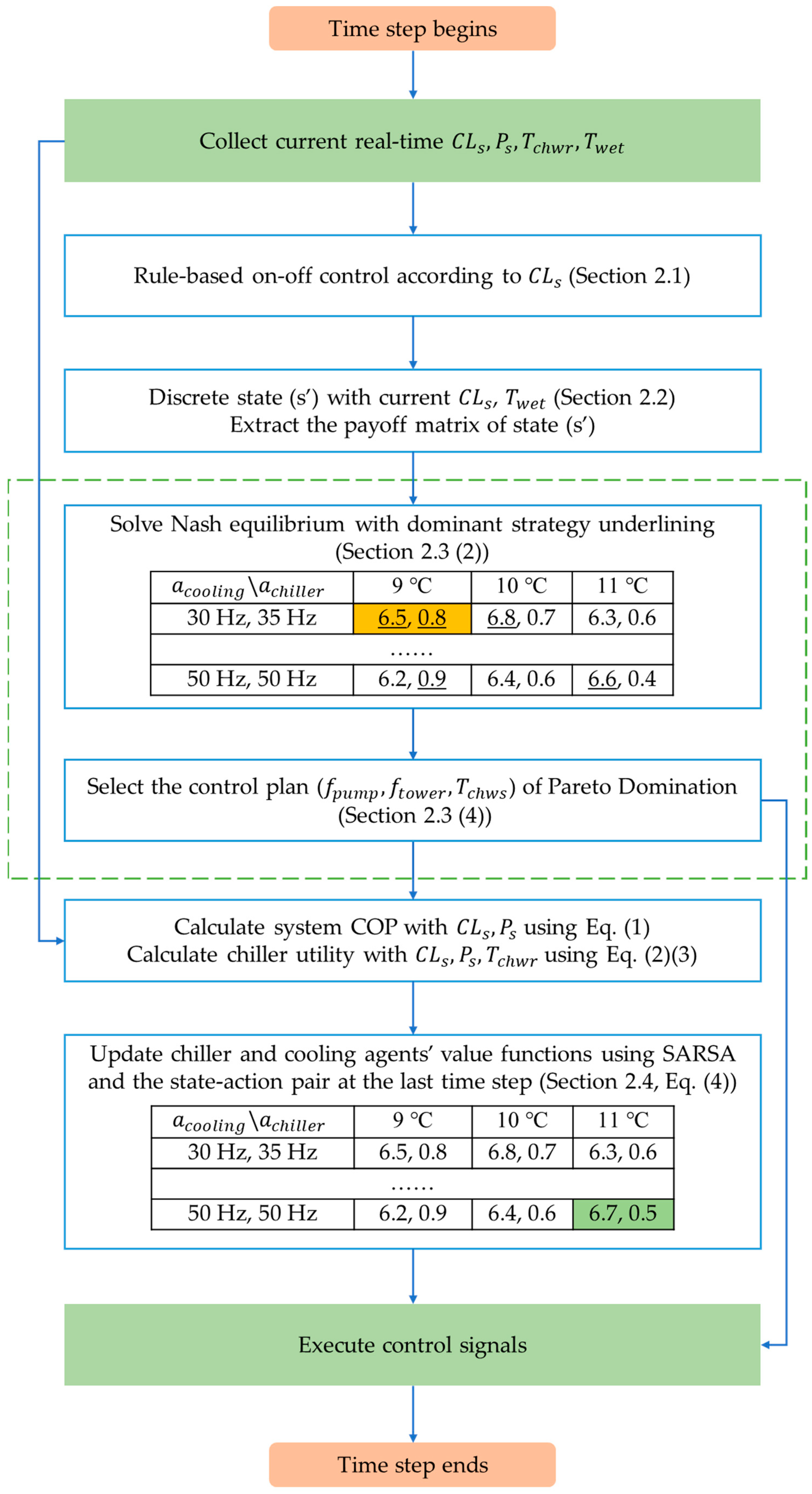
2.1. Overview
- (1)
- (2)
- All cooling towers operate simultaneously when the system is on to maximize heat exchange area [41].
- (3)
- Increase chiller running number only when is larger than current cooling capacity. Shutdown chiller(s) if fewer chillers still meet user’s cooling demand [8].
- (4)
- The number of running condenser and chilled water pumps is in accordance with the number of working chillers. Chilled water pump frequency is not optimized in this study.
2.2. RL Agent Formulation
2.3. Equilibrium Solving
- (1)
- In the beginning of every optimization time step, the system state is observed, and a certain matrix related to the current state (e.g., Table 2) can be extracted from the whole value function table (i.e., Table 1). In Table 2, (6.5, 0.8) means at current state, if cooling agent takes (30 Hz, 35 Hz) as the next action and chiller agent takes 9 as the next action, then their expected payoff would be 6.5 and 0.8, respectively.
- (2)
- Each agent underlines its optimal payoff for every potential action of the other agent. For instance (let us ignore the “…” part for now for simplicity), cooling agent needs to underline 6.5 in Table 2 because if chiller agent takes 9 at current time step, the maximal payoff (i.e., value function value) for the cooling agent would be 6.5, in accordance with its optimal action (30 Hz, 35 Hz). Similarly, cooling agent needs to underline 6.8 and 6.6 in case that chiller agent takes 10 or 11 . On the other hand, for the chiller agent, it needs to underline 0.8 and 0.9 in Table 2 because, according to the current value function table (i.e., Table 2), no matter which action is taken by cooling agent, chiller agent should take 9 to maximize its own payoff.
- (1)
- After underlining all optimal payoffs, find cells with two lines. In Table 2, there is one cell corresponding to a strategy set of (30 Hz, 35 Hz, 9 ), and this strategy set is a Nash equilibrium solution. If there are more than one strategy set, take the next step; otherwise the optimization of is competed with the only answer.
- (2)
- For matrix games with large strategy space (i.e., large action space of RL agents), there may be more than one Nash equilibrium solution. Under this circumstance, the proposed approach uses Pareto domination principle to refine the solutions [44]. Concretely, the proposed approach would compare all equilibrium solutions’ payoffs; if one solution’s payoff is dominated by anyone else, then this solution would be excluded. For instance, there are four solutions (i.e., four sets such as ) corresponding to four payoffs (6.6, 0.8), (6.6, 0.9), (6.8, 0.8) and (6.7, 0.9). In this case, (6.6, 0.8) is dominated by the other three; (6.6, 0.9) is dominated by (6.7, 0.9); while (6.8, 0.8) and (6.7, 0.9) do not dominate each other. Hence the two strategy sets of payoffs, (6.6, 0.8) and (6.6, 0.9), would be excluded from the alternatives. After the comparison above, the other two solutions remain as alternatives, and the solution with the maximal cooling agent payoff (which is (6.8, 0.8)) would be chosen as the optimal control action set; then the optimization of is complete.
2.4. Value Function Update with SARSA
2.5. Hyperparameter Setting
3. Simulation Case Study
3.1. Virtual Environment Establishment
3.2. Compared Control Algorithms
- (1)
- Typically the learning task in a MARL field can be categorized into fully cooperative task [49], fully competitive task [50] and non-fully cooperative (mixed) task. Among them, the mixed task is the most general and complicated task form. Different MARL algorithms could handle different types of tasks, WoLF-PHC is a universal algorithm that is capable of dealing with a non-fully cooperative (mixed) task [51], which is also the targeted problem in this study.
- (2)
- WoLF-PHC can work feasibly in heterogeneous multi-agent systems. That is, even if not all agents are embedded with the same learning algorithm, WoLF-PHC could still work normally [51].
- (3)
- WoLF-PHC does not require agent’s prior knowledge about the task, which is the same as the approach proposed in this study [52].
- (4)
4. Results and Discussion
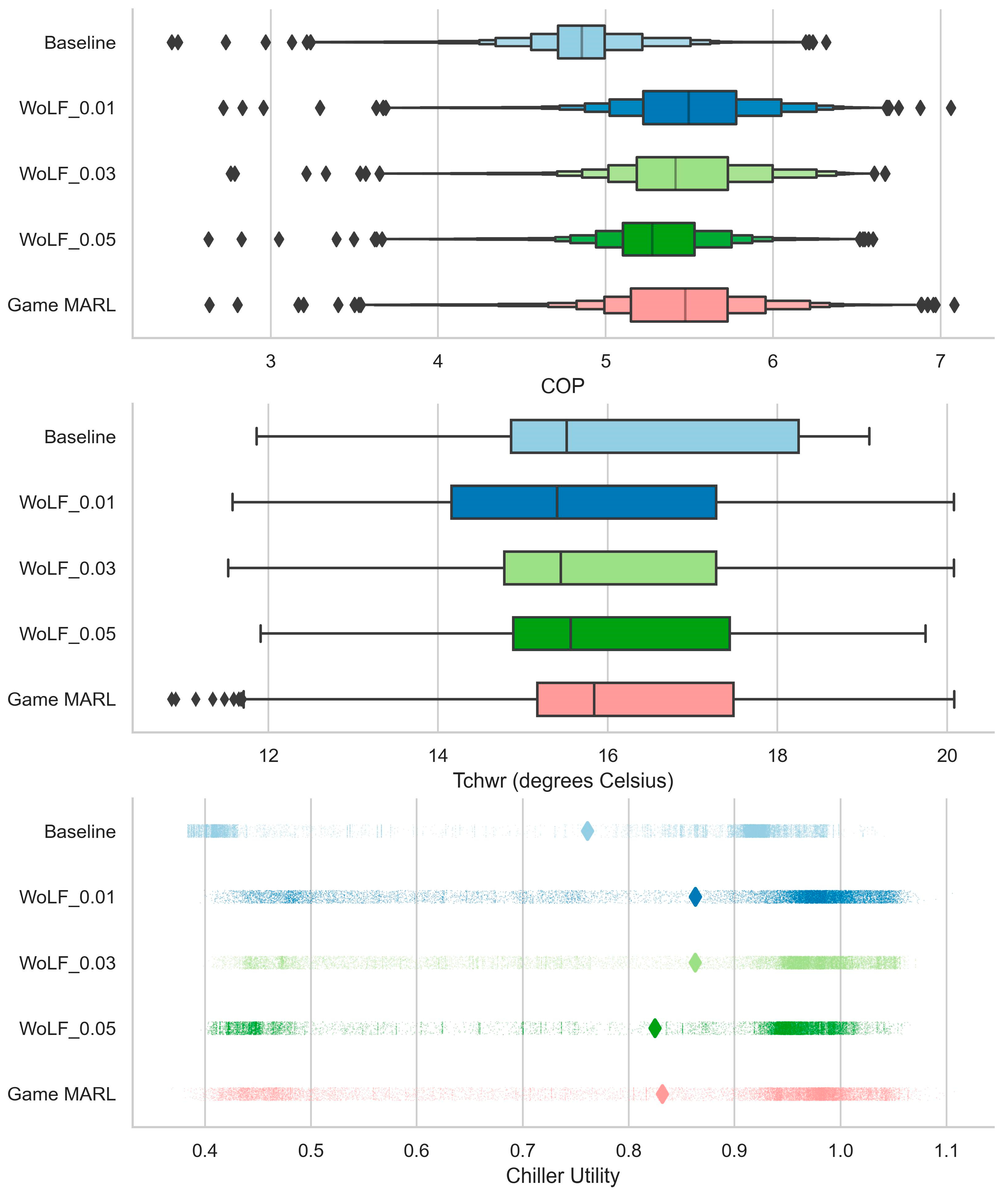
4.1. First Cooling Season Performance
4.2. Performance Evolution in Five Cooling Seasons
5. Conclusions and Future Work
5.1. Conclusions
5.2. Future Work
Author Contributions
Funding
Institutional Review Board Statement
Informed Consent Statement
Data Availability Statement
Conflicts of Interest
References
- Delmastro, C.; De Bienassis, T.; Goodson, T.; Lane, K.; Le Marois, J.-B.; Martinez-Gordon, R.; Husek, M. Buildings: Tracking Progress 2022; International Energy Agency: Paris, France, 2022. [Google Scholar]
- Wang, S.; Ma, Z. Supervisory and Optimal Control of Building HVAC Systems: A Review. Hvac R Res. 2008, 14, 3–32. [Google Scholar] [CrossRef]
- Commercial Buildings Energy Consumption Survey (CBECS). 2012 CBECS Survey Data; Commercial Buildings Energy Consumption Survey (CBECS): Washington, DC, USA, 2012.
- Taylor, S.T. Fundamentals of Design and Control of Central Chilled-Water Plants; ASHRAE Learning Institute: Atlanta, GA, USA, 2017. [Google Scholar]
- Qiu, S.; Li, Z.; Li, Z.; Wu, Q. Comparative Evaluation of Different Multi-Agent Reinforcement Learning Mechanisms in Condenser Water System Control. Buildings 2022, 12, 1092. [Google Scholar] [CrossRef]
- Chang, Y.C. A novel energy conservation method—Optimal chiller loading. Electr. Power Syst. Res. 2004, 69, 221–226. [Google Scholar] [CrossRef]
- Dai, Y.; Jiang, Z.; Wang, S. Decentralized control of parallel-connected chillers. Energy Procedia 2017, 122, 86–91. [Google Scholar] [CrossRef]
- Li, Z.; Huang, G.; Sun, Y. Stochastic chiller sequencing control. Energy Build. 2014, 84, 203–213. [Google Scholar] [CrossRef]
- Wang, L.; Lee, E.W.M.; Yuen, R.K.K.; Feng, W. Cooling load forecasting-based predictive optimisation for chiller plants. Energy Build. 2019, 198, 261–274. [Google Scholar] [CrossRef]
- Wang, J.; Hou, J.; Chen, J.; Fu, Q.; Huang, G. Data mining approach for improving the optimal control of HVAC systems: An event-driven strategy. J. Build. Eng. 2021, 39, 102246. [Google Scholar] [CrossRef]
- Wang, Y.; Jin, X.; Shi, W.; Wang, J. Online chiller loading strategy based on the near-optimal performance map for energy conservation. Appl. Energy 2019, 238, 1444–1451. [Google Scholar] [CrossRef]
- Hou, J.; Li, X.; Wan, H.; Sun, Q.; Dong, K.; Huang, G. Real-time optimal control of HVAC systems: Model accuracy and optimization reward. J. Build. Eng. 2022, 50, 104159. [Google Scholar] [CrossRef]
- Qiu, S.; Li, Z.; Fan, D.; He, R.; Dai, X.; Li, Z. Chilled water temperature resetting using model-free reinforcement learning: Engineering application. Energy Build. 2022, 255, 111694. [Google Scholar] [CrossRef]
- Zhu, N.; Shan, K.; Wang, S.; Sun, Y. An optimal control strategy with enhanced robustness for air-conditioning systems considering model and measurement uncertainties. Energy Build. 2013, 67, 540–550. [Google Scholar] [CrossRef]
- Azuatalam, D.; Lee, W.-L.; de Nijs, F.; Liebman, A. Reinforcement learning for whole-building HVAC control and demand response. Energy AI 2020, 2, 100020. [Google Scholar] [CrossRef]
- Henze, G.P.; Schoenmann, J. Evaluation of Reinforcement Learning Control for Thermal Energy Storage Systems. HVAC R Res. 2003, 9, 259–275. [Google Scholar] [CrossRef]
- Wang, Z.; Hong, T. Reinforcement learning for building controls: The opportunities and challenges. Appl. Energy 2020, 269, 115036. [Google Scholar] [CrossRef]
- Liu, S.; Henze, G.P. Experimental analysis of simulated reinforcement learning control for active and passive building thermal storage inventory. Part 2: Results and analysis. Energy Build. 2006, 38, 148–161. [Google Scholar] [CrossRef]
- Esrafilian-Najafabadi, M.; Haghighat, F. Towards self-learning control of HVAC systems with the consideration of dynamic occupancy patterns: Application of model-free deep reinforcement learning. Build. Environ. 2022, 226, 109747. [Google Scholar] [CrossRef]
- Crawley, D.B.; Lawrie, L.K.; Winkelmann, F.C.; Buhl, W.F.; Huang, Y.J.; Pedersen, C.O.; Strand, R.K.; Liesen, R.J.; Fisher, D.E.; Witte, M.J. EnergyPlus: Creating a new-generation building energy simulation program. Energy Build. 2001, 33, 319–331. [Google Scholar] [CrossRef]
- Li, W.; Xu, P.; Lu, X.; Wang, H.; Pang, Z. Electricity demand response in China: Status, feasible market schemes and pilots. Energy 2016, 114, 981–994. [Google Scholar] [CrossRef]
- Schreiber, T.; Eschweiler, S.; Baranski, M.; Müller, D. Application of two promising Reinforcement Learning algorithms for load shifting in a cooling supply system. Energy Build. 2020, 229, 110490. [Google Scholar] [CrossRef]
- Liu, X.; Ren, M.; Yang, Z.; Yan, G.; Guo, Y.; Cheng, L.; Wu, C. A multi-step predictive deep reinforcement learning algorithm for HVAC control systems in smart buildings. Energy 2022, 259, 124857. [Google Scholar] [CrossRef]
- Wang, D.; Gao, C.; Sun, Y.; Wang, W.; Zhu, S. Reinforcement learning control strategy for differential pressure setpoint in large-scale multi-source looped district cooling system. Energy Build. 2023, 282, 112778. [Google Scholar] [CrossRef]
- Qiu, S.; Li, Z.; Li, Z. Model-Free Optimal Control Method for Chilled Water Pumps Based on Multi-objective Optimization: Engineering Application. In Proceedings of the 2021 ASHRAE Virtual Conference, Phoenix, AZ, USA, 28–30 June 2021. [Google Scholar]
- Fu, Q.; Chen, X.; Ma, S.; Fang, N.; Xing, B.; Chen, J. Optimal control method of HVAC based on multi-agent deep reinforcement learning. Energy Build. 2022, 270, 112284. [Google Scholar] [CrossRef]
- Li, S.; Pan, Y.; Xu, P.; Zhang, N. A decentralized peer-to-peer control scheme for heating and cooling trading in distributed energy systems. J. Clean. Prod. 2021, 285, 124817. [Google Scholar] [CrossRef]
- Wang, Z.; Zhao, Y.; Zhang, C.; Ma, P.; Liu, X. A general multi agent-based distributed framework for optimal control of building HVAC systems. J. Build. Eng. 2022, 52, 104498. [Google Scholar] [CrossRef]
- Li, W.; Wang, S. A multi-agent based distributed approach for optimal control of multi-zone ventilation systems considering indoor air quality and energy use. Appl. Energy 2020, 275, 115371. [Google Scholar] [CrossRef]
- Li, W.; Li, H.; Wang, S. An event-driven multi-agent based distributed optimal control strategy for HVAC systems in IoT-enabled smart buildings. Autom. Constr. 2021, 132, 103919. [Google Scholar] [CrossRef]
- Li, S.; Pan, Y.; Wang, Q.; Huang, Z. A non-cooperative game-based distributed optimization method for chiller plant control. Build. Simul. 2022, 15, 1015–1034. [Google Scholar] [CrossRef]
- Homod, R.Z.; Yaseen, Z.M.; Hussein, A.K.; Almusaed, A.; Alawi, O.A.; Falah, M.W.; Abdelrazek, A.H.; Ahmed, W.; Eltaweel, M. Deep clustering of cooperative multi-agent reinforcement learning to optimize multi chiller HVAC systems for smart buildings energy management. J. Build. Eng. 2023, 65, 105689. [Google Scholar] [CrossRef]
- Zhang, K.; Yang, Z.; Baar, T. Multi-Agent Reinforcement Learning: A Selective Overview of Theories and Algorithms. arXiv 2019, arXiv:1911.10635. [Google Scholar] [CrossRef]
- Fudenberg, D.; Tirole, J. Game Theory, 1st ed.; The MIT Press: Cambridge, MA, USA, 1991; Volume 1. [Google Scholar]
- Myerson, R.B. Game Theory: Analysis of Conflict; Harvard University Press: Cambridge, MA, USA, 1997. [Google Scholar]
- Sun, S.; Shan, K.; Wang, S. An online robust sequencing control strategy for identical chillers using a probabilistic approach concerning flow measurement uncertainties. Appl. Energy 2022, 317, 119198. [Google Scholar] [CrossRef]
- Wang, J.; Huang, G.; Sun, Y.; Liu, X. Event-driven optimization of complex HVAC systems. Energy Build. 2016, 133, 79–87. [Google Scholar] [CrossRef]
- Ardakani, A.J.; Ardakani, F.F.; Hosseinian, S.H. A novel approach for optimal chiller loading using particle swarm optimization. Energy Build. 2008, 40, 2177–2187. [Google Scholar] [CrossRef]
- Lee, W.; Lin, L. Optimal chiller loading by particle swarm algorithm for reducing energy consumption. Appl. Therm. Eng. 2009, 29, 1730–1734. [Google Scholar] [CrossRef]
- Chang, Y.C.; Lin, J.K.; Chuang, M.H. Optimal chiller loading by genetic algorithm for reducing energy consumption. Energy Build. 2005, 37, 147–155. [Google Scholar] [CrossRef]
- Braun, J.E.; Diderrich, G.T. Near-optimal control of cooling towers for chilled-water systems. ASHRAE Trans. 1990, 96, 2. [Google Scholar]
- Zhao, Z.; Yuan, Q. Integrated Multi-objective Optimization of Predictive Maintenance and Production Scheduling: Perspective from Lead Time Constraints. J. Intell. Manag. Decis. 2022, 1, 67–77. [Google Scholar] [CrossRef]
- Qiu, S.; Feng, F.; Zhang, W.; Li, Z.; Li, Z. Stochastic optimized chiller operation strategy based on multi-objective optimization considering measurement uncertainty. Energy Build. 2019, 195, 149–160. [Google Scholar] [CrossRef]
- Matignon, L.; Laurent, G.J.; Le Fort-Piat, N. Independent reinforcement learners in cooperative Markov games: A survey regarding coordination problems. Knowl. Eng. Rev. 2012, 27, 1–31. [Google Scholar] [CrossRef] [Green Version]
- Rummery, G.; Niranjan, M. On-Line Q-Learning Using Connectionist Systems; Technical Report CUED/F-INFENG/TR 166; University of Cambridge, Department of Engineering: Cambridge, UK, 1994. [Google Scholar]
- Pedregosa, F.; Varoquaux, G.; Gramfort, A.; Michel, V.; Thirion, B.; Grisel, O.; Blondel, M.; Prettenhofer, P.; Weiss, R.; Dubourg, V.; et al. Scikit-learn: Machine Learning in Python. J. Mach. Learn. Res. 2011, 12, 2825–2830. [Google Scholar]
- Tao, J.Y.; Li, D.S. Cooperative Strategy Learning in Multi-Agent Environment with Continuous State Space; IEEE: New York, NY, USA, 2006; pp. 2107–2111. [Google Scholar]
- Xi, L.; Chen, J.; Huang, Y.; Xu, Y.; Liu, L.; Zhou, Y.; Li, Y. Smart generation control based on multi-agent reinforcement learning with the idea of the time tunnel. Energy 2018, 153, 977–987. [Google Scholar] [CrossRef]
- Lauer, M. An algorithm for distributed reinforcement learning in cooperative multiagent systems. In Proceedings of the 17th International Conference on Machine Learning, Stanford, CA, USA, 29 June–2 July 2000. [Google Scholar]
- Littman, M.L. Markov Games as a Framework for Multi-Agent Reinforcement Learning. In Machine Learning Proceedings 1994; Cohen, W.W., Hirsh, H., Eds.; Morgan Kaufmann: San Francisco, CA, USA, 1994; pp. 157–163. [Google Scholar]
- Buşoniu, L.; Babuška, R.; De Schutter, B. Multi-Agent Reinforcement Learning: An Overview, in Innovations in Multi-Agent Systems and Applications—1; Srinivasan, D., Jain, L.C., Eds.; Springer: Berlin/Heidelberg, Germany, 2010; pp. 183–221. [Google Scholar]
- Bowling, M.; Veloso, M. Multiagent learning using a variable learning rate. Artif. Intell. 2002, 136, 215–250. [Google Scholar] [CrossRef] [Green Version]
- Xi, L.; Yu, T.; Yang, B.; Zhang, X. A novel multi-agent decentralized win or learn fast policy hill-climbing with eligibility trace algorithm for smart generation control of interconnected complex power grids. Energy Convers. Manag. 2015, 103, 82–93. [Google Scholar] [CrossRef]
- Qiu, S.; Li, Z.; Li, Z.; Zhang, X. Model-free optimal chiller loading method based on Q-learning. Sci. Technol. Built Environ. 2020, 26, 1100–1116. [Google Scholar] [CrossRef]


| 24 °C, 1060 kW | 25 °C, 1060 kW | 28 °C, 2120 kW | |||
|---|---|---|---|---|---|
| 9 °C | 10 °C | 11 °C | |||
| 30 Hz, 35 Hz | 6.5, 0.8 | 6.8, 0.7 | 6.3, 0.6 | ||
| …… | …… | ||||
| 50 Hz, 50 Hz | 6.2, 0.9 | 6.4, 0.6 | 6.6, 0.4 | ||
| 30 Hz, 35 Hz | 6.5, 0.8 | 6.8, 0.7 | 6.3, 0.6 |
| …… | …… | ||
| 50 Hz, 50 Hz | 6.2, 0.9 | 6.4, 0.6 | 6.6, 0.4 |
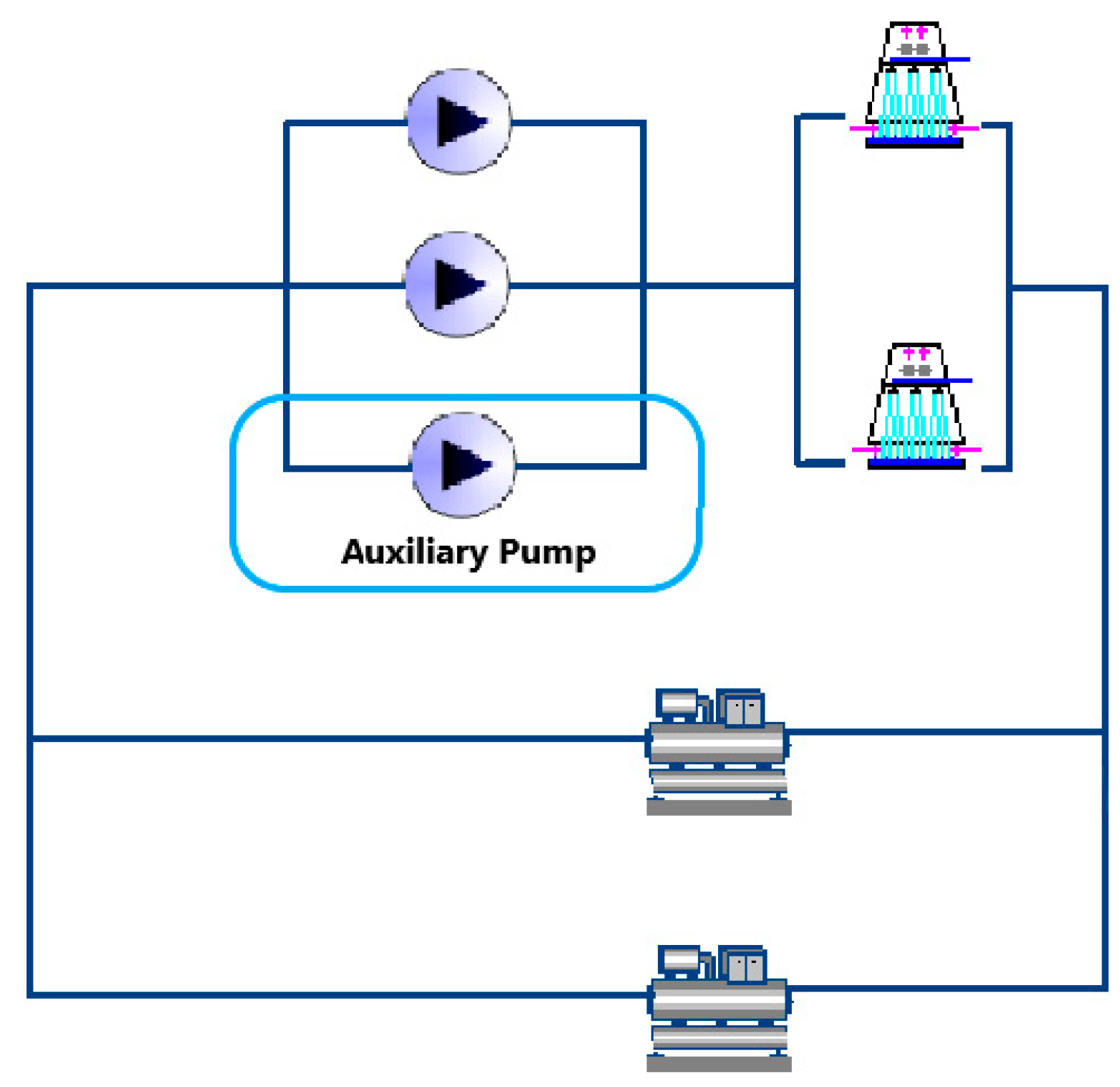
| Equipment | Number | Characteristics (Single Appliance) |
|---|---|---|
| Screw chiller | 2 | Cooling capacity = 1060 kW, power = 159.7 kW Chilled water temperature = 10/17 °C Chilled water flow rate = 131 m3/h (36.39 kg/s) |
| Condenser water pump | 2 + 1 (one auxiliary) | Power = 14.7 kW, flowrate = 240 m3/h Head: 20 m, variable speed |
| Cooling tower | 2 | Power = 7.5 kW, flowrate = 260 m3/h, variable speed |
| Variable | Description | Unit |
|---|---|---|
| Real-time overall electrical power of chillers, condenser water pumps and cooling towers | kW | |
| System cooling load | kW | |
| Ambient wet-bulb temperature | ||
| Common frequency of running condenser water pump(s) | Hz | |
| Current working number of condenser water pumps (equal to the running number of chillers and chilled water pumps) | ||
| Working frequency of running cooling tower(s) | Hz | |
| Current working number of cooling towers | ||
| Temperature of supplied chilled water | ||
| Temperature of returned chilled water | ||
| Nominal chilled water flowrate of single chiller | kg/s | |
| Specific heat capacity of water | kJ/(kg·K) | |
| Current working status of chillers: 1–only Chiller 1 is running, 2–only Chiller 2 is running, 3–both chillers are running, 0–no chiller is running |
| Case | Controller Algorithm | Cooling Tower Action | Condenser Pump Action | Chiller Action | Parameters | State | Reward |
|---|---|---|---|---|---|---|---|
| 1 | Baseline | 50 Hz | 50 Hz | 10 °C | / | / | / |
| 2 | WoLF-PHC | 30, 35, 40, 45, 50 Hz | 35, 40, 45, 50 Hz | 9, 10, 11 °C | , | System COP, chiller utility | |
| 3 | |||||||
| 4 | |||||||
| 5 | Game theory MARL | Jointed action-like (pump 50 Hz, tower 30 Hz) | 9, 10, 11 °C | ||||
| Case | Total energy Consumption (kWh) | Cumulated Chiller Utility |
|---|---|---|
| 1 | 549,101 | 11,511.58 |
| 2 | 486,865 | 13,055.17 |
| 3 | 490,685 | 13,052.78 |
| 4 | 505,180 | 12,474.10 |
| 5 | 491,623 | 12,579.88 |
Disclaimer/Publisher’s Note: The statements, opinions and data contained in all publications are solely those of the individual author(s) and contributor(s) and not of MDPI and/or the editor(s). MDPI and/or the editor(s) disclaim responsibility for any injury to people or property resulting from any ideas, methods, instructions or products referred to in the content. |
© 2023 by the authors. Licensee MDPI, Basel, Switzerland. This article is an open access article distributed under the terms and conditions of the Creative Commons Attribution (CC BY) license (https://creativecommons.org/licenses/by/4.0/).
Share and Cite
Qiu, S.; Li, Z.; Pang, Z.; Li, Z.; Tao, Y. Multi-Agent Optimal Control for Central Chiller Plants Using Reinforcement Learning and Game Theory. Systems 2023, 11, 136. https://doi.org/10.3390/systems11030136
Qiu S, Li Z, Pang Z, Li Z, Tao Y. Multi-Agent Optimal Control for Central Chiller Plants Using Reinforcement Learning and Game Theory. Systems. 2023; 11(3):136. https://doi.org/10.3390/systems11030136
Chicago/Turabian StyleQiu, Shunian, Zhenhai Li, Zhihong Pang, Zhengwei Li, and Yinying Tao. 2023. "Multi-Agent Optimal Control for Central Chiller Plants Using Reinforcement Learning and Game Theory" Systems 11, no. 3: 136. https://doi.org/10.3390/systems11030136