Parallel Learning of Dynamics in Complex Systems

Abstract

Dynamics always exist in complex systems. Graphs (complex networks) are a mathematical form for describing a complex system abstractly. Dynamics can be learned efficiently from the structure and dynamics state of a graph. Learning the dynamics in graphs plays an important role in predicting and controlling complex systems. Most of the methods for learning dynamics in graphs run slowly in large graphs. The complexity of the large graph’s structure and its nonlinear dynamics aggravate this problem. To overcome these difficulties, we propose a general framework with two novel methods in this paper, the Dynamics-METIS (D-METIS) and the Partitioned Graph Neural Dynamics Learner (PGNDL). The general framework combines D-METIS and PGNDL to perform tasks for large graphs. D-METIS is a new algorithm that can partition a large graph into multiple subgraphs. D-METIS innovatively considers the dynamic changes in the graph. PGNDL is a new parallel model that consists of ordinary differential equation systems and graph neural networks (GNNs). It can quickly learn the dynamics of subgraphs in parallel. In this framework, D-METIS provides PGNDL with partitioned subgraphs, and PGNDL can solve the tasks of interpolation and extrapolation prediction. We exhibit the universality and superiority of our framework on four kinds of graphs with three kinds of dynamics through an experiment.

1. Introduction

Complex networks or graphs are ubiquitous in life, and each individual is a node or vertex in many kinds of graphs. It is very important to know what complex networks are and how they affect us. Many systematic problems can be constructed as the mathematical tool of a ‘Graph’ to carry out research and solve many practical problems, such as the global outbreak of the WannaCry computer blackmail virus [1], the COVID-19 global pandemic [2], the rapid spread of monkeypox [3], and the spread of rumors in social networks [4]. All of these can be modeled as a graph or a complex network model. For these complex systems, constructing effective graph models is helpful for better predictions and control. Specifically, graphs help us to prevent the spread of epidemics, block the spread of computer viruses, crack down on terrorist networks [5], improve the robustness of power grids, strengthen public opinion monitoring, and so on. Dynamics is a mainstream approach for studying the dynamic processes of vertexes in a graph. There are now many studies on network dynamics [6], and the existing dynamics models of graphs are still worthy of further study. Dynamics makes the solution to the dynamic process of the network easily explainable. Nonlinear dynamics models have been widely studied and applied in different fields, including applied mathematics [7,8], statistical physics [9], and engineering [10]. Some networks’ evolution mechanisms are known at the beginning of their establishment, but the real world is so complex that the potential dynamics of a large number of complex networks are unknown. It is difficult to construct complex models of these unknown differential equations. Dynamics modeling on a graph also becomes more challenging when considering the unknown elements of dynamics and the large scale of the complex system itself.

Fortunately, in the era of big data, many complex network systems have produced a large amount of available data in the process of dynamic development. When seeking a model for the data, we can learn its dynamics on a graph with a combination of ODEs and GNNs. In addition, after the complex system is abstracted into a graph, its complex network structure, large-scale edges and vertexes, and complex dynamics processes form a series of NP-complete problems [11,12]. This results in the poor performance of many models and algorithms on the graph. However, there is a better method, namely, graph partition. This process evenly divides the large-scale graph into a series of subgraphs to adapt to distributed applications. Therefore, the learning process of the dynamics on a graph can be accelerated by graph partition. Based on this, we proposed a model framework for graph partition to accelerate the graph neural dynamics learning process. This method skillfully combines the dynamic process on the graph with the fast graph-partition algorithm METIS and realizes a large-scale graph-partition method considering a dynamic process. After the large graph is divided evenly, the dynamics of each subgraph can further be learned in parallel by combining GNNs [13,14,15,16] and differential equations. This helps us to recognize, predict, and control a complex system more quickly and accurately.

Our work can be used for two tasks in a general framework. One is partitioning a large graph with network dynamics for parallel tasks downstream. Another is learning the unequal time interval states of subgraph dynamics for interpolation and extrapolation predictions. In task one, this model is more accurate and faster than the usual spectral clustering; the execution efficiency is very high, i.e., one to two orders of magnitude faster than the common partition algorithm; and a graph with millions of vertexes can be divided into 256 classes in a few seconds. In task two, the model can learn unequal interval (continuous-time) dynamics in graphs. It obtains more accurate results than most graphs and dynamics, and it is more than twice as fast as other models.

Overall, the main contributions of this paper are as follows:

(1)

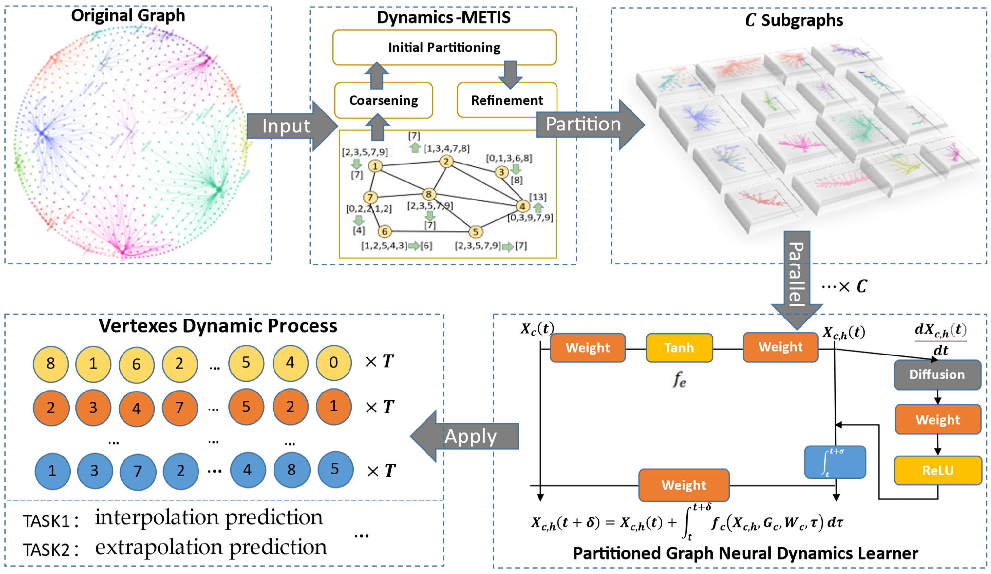
A novel algorithm: We propose a novel algorithm for graph partition, namely, Dynamics-METIS (D-METIS). D-METIS can partition a large graph into multiple subgraphs, and it innovatively considers two balances of the subgraphs, i.e., the balance of vertexes and the balance of cumulative dynamic changes.

(2)

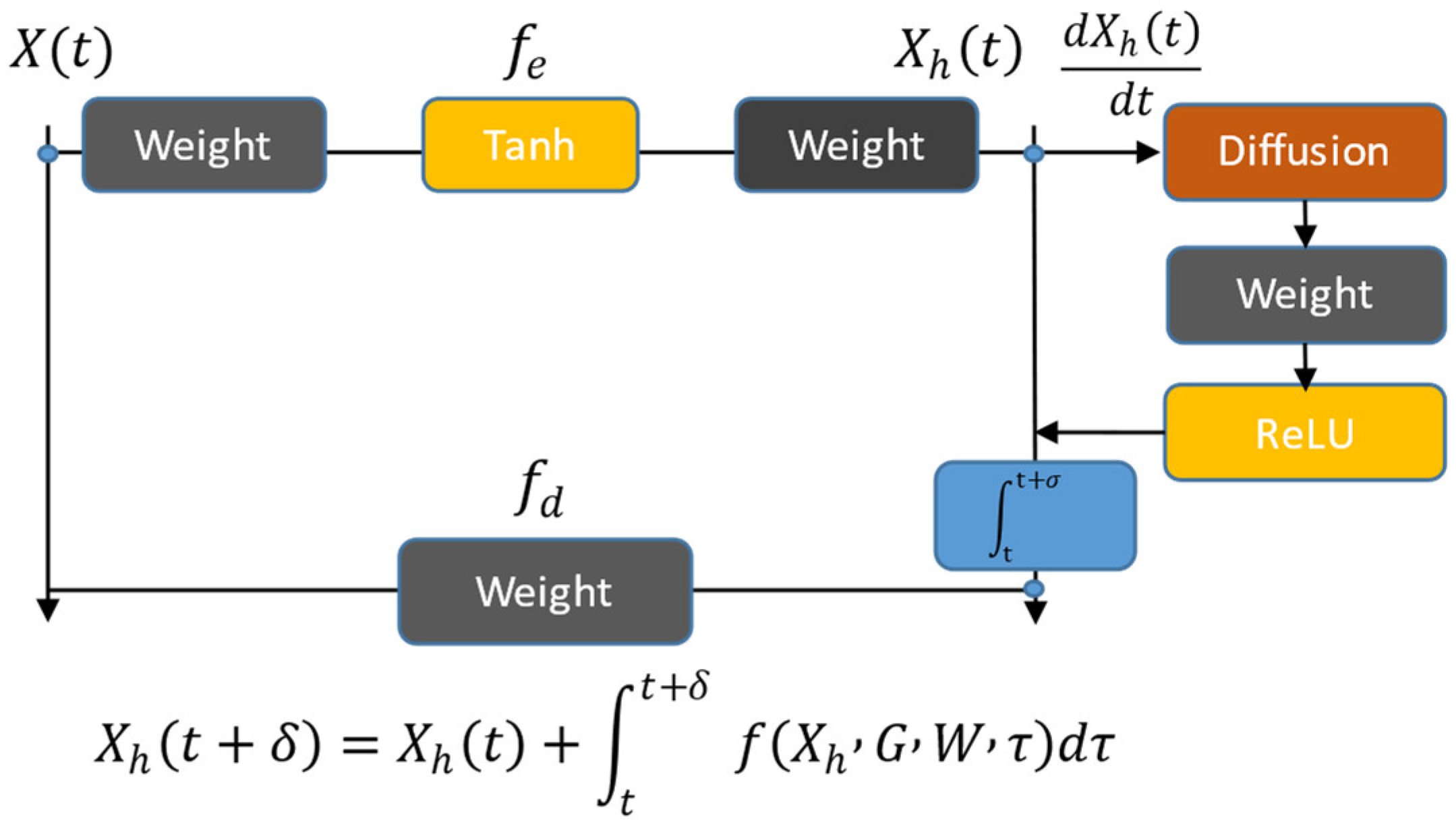
A novel model: This novel model is called the Partitioned Graph Neural Dynamics Learner (PGNDL). The PGNDL is a parallel model that combines ordinary differential equation systems and GNN. Thus, it can quickly learn the dynamics of large graphs. It can also learn unequal interval (continuous-time) dynamics on any graph.

(3)

More efficient parallel general framework: The experimental results show that our framework completed the tasks on various graphs faster than the most well-known framework, NDCN [17], with at least twice the efficiency.

(4)

More accurate in regression tasks: The PGNDL (D-METIS) performs accurately on various dynamics and networks.

The main purpose of this paper is to accelerate the dynamics learning process on large graphs, apply the graph-partition algorithm to cut large graphs into needed subgraphs, and then implement the neural dynamics learning model in parallel in each subgraph. Compared to the existing method of graph partition, our model can learn more complex dynamics on larger graphs and achieve faster, more accurate, and more interpretable results. Our D-METIS considers not only the balance of the number of nodes in each subgraph but also the balance of the degree of dynamic changes in each subgraph. Additionally, our PGNDL model is different from other existing GNNs [14,15,16,17]. It is a parallel learning method, which can reduce the complexity of each thread and improve the computational efficiency.

To illustrate the proposed framework, we review knowledge of graph partition and GNNs with ODE (Section 2). Then, we define the methods and framework’s terminology and its algorithms (Section 3). Following this, we demonstrate the framework on different graphs with different dynamics using 24 datasets consisting of 400 vertexes and 2000 vertexes (Section 4). Finally, we summarize this work (Section 5).

2. Related Work

2.1. Graph Partition

Graph partitioning involves evenly dividing a large graph into a series of subgraphs. This means subgraphs can be executed in parallel. If the current subgraph needs information from other subgraphs, partitioning must consider information transfer. The quality of the graph partition affects the storage cost of each machine and the communication cost among machines. According to the memory cost of partition, it can be divided into offline and streaming partition algorithms. For large-scale graph data, streaming partition is particularly important when the memory of a single machine cannot meet the requirements of the partition algorithm [18]. The partition method of graph data can be divided into vertex partitioning or edge-cut partitioning. For graph data with power law distribution, some vertexes may have many edges; if we run the vertex partitioning, many edges will be missing, and the edge load will be uneven, but edge partition can deal with this kind of problem [19]. The two goals of graph partition are load balancing (reducing storage costs) and minimizing cuts (reducing communication costs). At the same time, the two goals of optimization are balanced graph partitioning.

As you can see, graph partition is an NP-hard problem [19]. In normal circumstances, the relaxation is to optimize load balancing and ensure minimum cuts as much as possible. We can define a Graph as $G=\left(V,E\right)$, which means graph $G$ has $\left|V\right|$ vertexes and $\left|E\right|$ edges.

The edge partitioning is shown as follows:

$$\underset{i\in \left[1,k\right]}{max}\left|E_i\right|\le \frac{\left(1+\alpha \right)\left|E\right|}{k}$$

(1)

$$R{F}_v={\displaystyle \sum }_{i-1}^k\frac{V\left(E_i\right)}{\left|V\right|}$$

(2)

In Formula (1), the balanced graph-partitioning problem is defined as creating $k$ disjoint sets of vertices (partitions); $\left|E\right|$ means the number of edges in graph G; $V\left(E_i\right)$ means a set of vertexes representing the association of all edges $E_i$ in a subgraph; and the parameter $\alpha$ controls the balance rate. In Formula (2) $R{F}_v$ represents the replication factor of the vertex and measures the number of vertex cuts. Regarding edge partition, linear deterministic greedy partitioning (LDG) [18] considers using a greedy algorithm to put neighbor vertexes together during partition to reduce edge cutting and ensure the vertex load balance of each subgraph. Compared with LDG, Fennel’s [20] scoring function has relaxed the constraint on the number of vertexes in the subgraph from multiplication to subtraction. METIS [21] is a hierarchical partitioning algorithm. The core idea is to reduce the size of the original graph via continuously sparsely merging vertexes and edges for a given original graph structure and then, to a certain extent, segmenting the reduced graph structure. Finally, the small, segmented graph is restored to the original graph structure to ensure the balance of each subgraph. METIS adopts the heavy edge-matching strategy in the sparse phase. When dividing the reduced subgraph, it randomly initializes a node to conduct a width first search to obtain the subgraph with the minimum tangent edge and then maps it to the original graph structure. Because METIS needs to traverse and scale the entire graph structure, it is inefficient when segmenting large-scale graphs with large memory consumption.

Additionally, the edge partitioning is as follows:

$$\underset{i\in \left[1,k\right]}{max}\left|V_i\right|\le \frac{\left(1+\alpha \right)\left|V\right|}{k}$$

(3)

where $\left|V_i\right|$ means the number of vertexes in each subgraph, representing the load balancing of the vertex; and the parameter $\alpha$ controls the balance rate. Regarding edge partition, neighbor expansion (NE) [19] edge partition also considers the locality of neighbors; for the boundary vertex, it selects a candidate vertex whose neighbor is the closest to the outside of the boundary, which can ensure the maximization of the assigned neighbor edge to ensure the minimum node-repetition rate. Degree-Based Hashing (DBH) [22] divides the vertex allocation edge by judging the degree information of the vertex. For power-law graphs, the locality of low-degree vertexes is easy to maintain. Meanwhile, for high-degree vertexes, it is impossible to allocate all edges on a subgraph because there are too many vertexes associated. Thus, the algorithm tries to maintain the locality of low-degree vertexes as much as possible. Additionally, the generalizable approximate graph-partitioning (GAP) framework [23] is a vertex-partition algorithm based on GNN.

2.2. GNNs with ODE

This is a new way to combine Ordinary Differential Equations (ODE) [17,24,25,26] and GNNs to learn the non-linear and high-dimensional dynamics of graphs. Neural Dynamics on Complex Networks (NDCN) [17] is a successful network class. NDCN captures the instantaneous rate of change of vertex states by differential equation systems and GNNs instead of mapping through a discrete number of layers forward. It integrates GNN layers in continuous time rather than discrete depth. The continuous-time dynamics on a graph can describe by a differential equation system, such as Formula (4).

$$\frac{dX\left(t\right)}{dt}=f\left(X,G,W,t\right)$$

(4)

where $X\left(t\right)\in {ℝ}^{v\times d}$ represents the state of a dynamic system consisting of $v$-linked vertexes at time $t\in \left[0,\infty \right)$, and $X\left(0\right)$ is the initial state of this system at time $t=0$. Each vertex is characterized by $v$ dimensional features. $G=\left(V,E\right)$ is the network structure capturing how vertexes interact with each other. $W\left(t\right)$ are parameters that control how the system evolves. The function $f$ governs the instantaneous rate of change of dynamics on the graph. We can obtain the NDCN model as follows:

$$\underset{W\left(t\right),\mathsf{\Theta }\left(T\right)}{\arg min} ℒ={{\displaystyle \int }}_0^T\mathcal{R}\left(X,G,W,t\right)dt+\mathcal{S}\left(Y\left(X\left(T\right),\mathsf{\Theta }\right)\right)$$

(5)

$$\begin{array}{c}subject to X_h\left(t\right)=f_e\left(X\left(t\right),W_e\right)\\ \frac{d{X}_h\left(t\right)}{dt}=f\left(X_h,G,W_h,t\right)\\ X\left(t\right)=f_d\left(X_h\left(t\right),W_d\right)\end{array}$$

(6)

where ${{\displaystyle \int }}_0^Tℛ\left(X,G,W,t\right)dt$ is the ‘running‘ loss of the continuous-time dynamics on graphs from t = 0 to T, and $\mathcal{S}\left(Y\left(X\left(T\right),\mathsf{\Theta }\right)\right)$ is the ‘terminal’ loss at time T. Vertexes can have various semantic labels encoded by one-hot encoding $Y\left(X\left(T\right),\mathsf{\Theta }\right)$, and Θ represents the parameters of this classification function. The first constraint transforms $X\left(t\right)$ into hidden space $X_h\left(t\right)$ through encoding function $f_e$, and $X\left(0\right)=X_0$. The second constraint is the governing dynamics in the hidden space. The third constraint decodes the hidden signal back to the original space with a decoding function.

The neural structures of the model are illustrated in Figure 1.

We can see that the input of NDCN is the node state $X\left(t\right)$ at time $t$, while the output is the node state after time $\left(t+\delta \right)$. The NDCN will first map the input X(t) into the hidden space using $X_h\left(t\right)$ to represent $X\left(t\right)$ after the hidden layer. The hidden layer is an encoding function $f_e$. Additionally, the dynamics of influence and information diffusion between nodes are modeled in the hidden space, which is completed through the GNN. By integrating the dynamic process $X_h\left(t\right)$ from t to t + δ, we can obtain the output state. Then, we use the decoder $f_d$ to obtain the status of nodes in the original space. Moreover, $f_e$ and $f_d$ are flexible as any deep neural structure (including the linear weighting layer and activation function).

From the point of view of the dynamic system, continuous depth can be interpreted as continuous physical time, and the output of any hidden GNN layer at time t is the instantaneous network dynamics process of conventional neural network models. Additionally, a unified framework for automated interactions and dynamics discovery (AIDD) was proposed [27]. It is based on the more rigorous mathematical form of Markov dynamics and local network interaction to express the problem. Additionally, it provides a unified objective function based on logarithmic likelihood. This kind of model has been applied to many fields, such as climate studies [28], rumor detection [29], and healthcare [30].

3. Methodology

Cutting a graph with dynamic characteristics is a new problem. Additionally, finding a graph-partition method that can match the downstream applications and how to dynamically reconstruct each subgraph are two difficulties inherent in this problem. The following methods and frameworks are proposed to resolve this problem.

In this section, we propose the Dynamics METIS (D-METIS) algorithm to solve the first difficulty of the problem. For the second difficulty, we use the data-driven method based on GNNs to obtain the dynamics of subgraphs cut by D-METIS, called the Partitioned Graph Neural Dynamics Learner (PGNDL), and we give its application ways to resolve the regression task of interpolation prediction and extrapolation prediction. Finally, we elaborate on the general framework.

3.1. Dynamics METIS

We proposed a novel method named Dynamics METIS (D-METIS) for cutting large graphs while considering the dynamics in the graph. There are three given rules when designing D-METIS:

• The graph structure damage caused by partitioning should be minimized;
• The structure of each subgraph should be evenly distributed to facilitate the synchronization and parallel assessment of downstream tasks;
• The distribution of the dynamics state change degree of each subgraph should be even and convenient for downstream application and analysis.

Thus, our D-METIS method can compress the dynamics states for more efficient graph-partitioning tasks and also take advantage of the information on state changes of vertexes, which takes the partitioning task closer to reality.

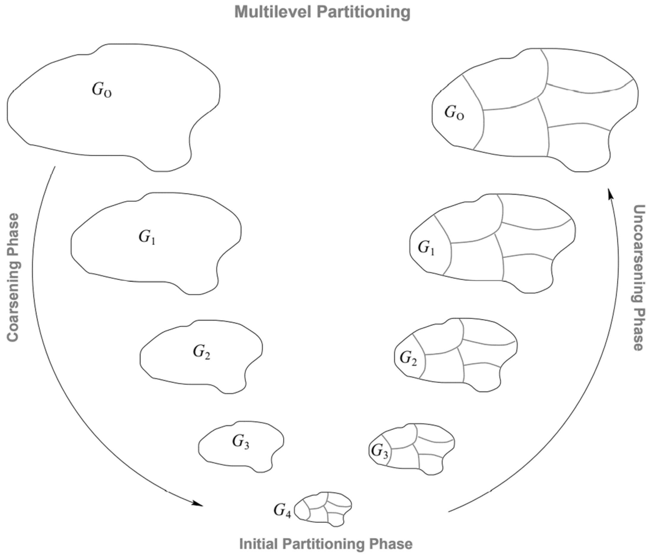
3.1.1. METIS Algorithm

METIS is a multilevel k-way partition algorithm [21]. The graph $G=\left(V,E\right)$ is first coarsened into a small-scale graph, which contains a small number of points. Then, the k-path is divided for the coarsened graph. At this time, the number of points is greatly reduced due to the coarsening, so a much smaller graph needs to be divided now, and the time complexity is greatly reduced. After the partition, each subgraph is refined step-by-step until the number of original points is restored to obtain the original graph. The three steps of coarsening, dividing, and refining can be seen graphically in Figure 2.

3.1.2. METIS for a Graph with Dynamics

The traditional METIS algorithm is applied to some static graphs without dynamics. However, there are many graphs with dynamics in the real world, so we need a new method for partitioning with dynamics. We enabled the METIS algorithm to be suitable for a graph with dynamics by designing the dynamic process compression strategy of vertexes. First, we give a case of dynamic process compression on a graph, as shown in Figure 3; in Figure 3a, we give every vertex five states; and in Figure 3b, we sequentially compute the sum of dynamic changes for each vertex as the new weight for vertexes. For example, the vertex numbered 1 has five states: 2→3→5→7→9, and is then compressed into a weight = 7. This compression method will be mathematically detailed later.

Let $G=\left(V, E\right)$ denote an undirected graph consisting of a vertex set $V$ and an edge set $E$. A pair of vertexes makes up an edge $\left(\mathrm{i}.\mathrm{e}., e=\left\{v_1, v_2\right\}\mathrm{where}{v}_1, v_2 \in V\right)$. The number of vertexes in the graph is denoted as $n=\left|V\right|,$ and the number of edges is denoted by $m=\left|E\right|$.

Additionally, vertexes can have a group of weights $v_i\left(t\right)$. $\mathrm{where} i\in \left(1, 2 ,3, \dots ,n\right),v_i\in V, t\in \left[0,T\right].$ If there are no weights specified on vertexes, they are assumed to be one.

To facilitate the partitioning of graphs with dynamics, the total dynamic change of vertexes is counted as the new unique weight of vertexes denoted by $w_i$ and is calculated as Formula (7).

$$w_i={\displaystyle \sum }_{t=0}^T\left|v_i\left(t\right)-v_i\left(t+1\right)\right|$$

(7)

Therefore, referring to the original steps of the METIS algorithm [21], the steps of our D-METIS algorithm are as follows:

• Obtaining graph data;
• Compressing dynamics process information;
• Converting the adjacency matrix to Compressed Sparse Row (CSR) format;
• Coarsening;
• Initial partitioning;
• Refinement.

This is a model for large graph partition with its dynamic changes. The balanced graph-partitioning problem is defined as creating $C$ disjoint sets of partitions, $V=V_1 \cup V_2 \dots \cup V_C$, with the constraint that the sum of the weights in any given set does not exceed some threshold $\epsilon$, which is greater than the average weight of a set $V_c$.

$$C\frac{\underset{c}{max}\left|V_c\right|}{\left|V\right|}\le 1+\epsilon$$

(8)

D-METIS’s objective is to minimize the weight of inter-partition edge $edgecuts$ while not exceeding the balance constraint.

$$edgecuts={\displaystyle \sum }_{c=1}^C{\displaystyle \sum }_{v\in V_c}{\displaystyle \sum }_{u\in \mathsf{\Gamma }\left(v\right),u\notin V_c}\mathsf{\theta }\{v,u\}$$

(9)

$${\displaystyle \sum }_{c=1}^C{G}_c+relink\left(edgecuts\right)=G$$

(10)

where $v, u\in V, c\in \left\{1, 2, 3, \dots ,C\right\},V_c\subseteq V$. The links between vertexes and the vertexes in each $V_c$ form a subgraph $G_c$. $relink\left(edgecuts\right)$ is a function for relinking all the cut edges between subgraphs; it turns the subgraphs into the original large graph $G$.

The specific value of $C$ depends on downstream task requirements. A larger value can be taken for faster results, and a smaller value can be used for improved accuracy. As we determined after many experiments, $C=\left|V\right|/l$, $l\in \left(100, 400\right), C\ge 2$ is best.

3.2. Partitioned Graph Neural Dynamics Learner

The Partitioned Graph Neural Dynamics Learner (PGNDL) is a model of learning dynamics on partitioned graphs. It is a parallel model proposed specifically for large graphs. First of all, we used a differential equation system, as presented in Formula (11), to describe the dynamics on subgraphs cut by D-METIS.

$$\frac{d{X}_c\left(t\right)}{dt}=f_c\left(X_c,G_c,W_c,t\right)$$

(11)

where $X_c\left(t\right)\in {ℝ}^{v\times d}$ represents the state of a dynamic system consisting of $v$-linked vertexes in the subgraph $G_c$ at time $t\in \left[0,T\right]$. $W_c\left(t\right)$ are parameters that control how the system evolves. The function $f_c$ governs the instantaneous rate of change of dynamics on the subgraph $G_c$.

Such a problem can be seen as an optimal control problem so that the goal becomes to learn the best control parameters $W_c\left(t\right)$ for Formula (11). Unlike the traditional optimal control modeling, we modeled Formula (10) using GNN. After integrating Formula (11) over continuous time, the graph neural ODE model was proposed, illustrated as Formula (12).

$$X_c\left(t\right)=X_c\left(0\right)+{{\displaystyle \int }}_0^t{f}_c\left(X_c,G_c,W_c,\tau \right)d\tau$$

(12)

Formula (11) can have continuous layers with a real number $t$ depth corresponding to the continuous-time dynamics on subgraph $G_c$. Thus, it can also be interpreted as a continuous-time GNN; the concept of continuous-time GNN was elaborated on in [17]. To increase the express ability of this model, we can encode the subgraph signals $X_c\left(t\right)$ from the original space to hidden space signals $X_{c,h}\left(t\right)$ so that this model can learn the dynamics better in a hidden space.

Then, a general model of graph neural dynamics learner can be denoted as follows:

$$\underset{W\left(t\right)}{\arg min}ℒ={\displaystyle \sum }_{c=1}^C \left({{\displaystyle \int }}_0^Tℛ\left(X_c,G_c,W_c,t\right)dt\right)$$

(13)

Subject to

$$X_{c,h}\left(t\right)=f_e\left(X_c\left(t\right),W_{c,e}\right)$$

(14)

$$\frac{d{X}_{c,h}\left(t\right)}{dt}=f\left(X_{c,h},G_c,W_{c,h},t\right)$$

(15)

$$X_c\left(t\right)=f_d\left(X_{c,h}\left(t\right),W_{c,d}\right)$$

(16)

where the objective formula, Formula (13), means the total loss of the continuous-time dynamics on subgraphs {$G_1, G_2, G_3,\dots \dots \dots ,G_C$} from $t=0 \mathrm{to} t=T$. The constraint formula, Formula (14), transforms $X_c\left(t\right)$ into hidden space $X_{c,h}\left(t\right)$, and $f_e$ is the encoding function. The constraint formula, Formula (15), is the governing dynamics in the hidden space by $f$. The constraint formula, Formula (16), decodes the hidden signal back to the original space by decoding function $f_d$. Additionally, $f_e$, $f$, and $f_d$ are flexible to be any deep neural structures.

The PGNDL can learn differential equation systems to predict unequal interval states of the vertex, which means the PGNDL can learn the continuous-time dynamics on a graph (or subgraphs) at an arbitrary physical time $t$. The arbitrary physical times mean is unequally sampled with different observational time intervals. Additionally, there are two situations: when $t<T$ and $t$ is not in $\left\{t, t+a, t+2a, \dots \right\}$ ($a$ is the value of equal sampling interval), it can be called interpolation prediction; when $t>T$, it is called extrapolation prediction.

We used ℓ1-norm loss as the loss function of the continuous-time dynamics on subgraphs and adopted two fully connected neural layers with a nonlinear hidden layer as $f_e$. A GCN model with a simplified diffusion operator $\mathsf{\Phi }$ denotes the instantaneous rate of dynamics changes on subgraphs in the hidden space, and $f_d$ is a linear decoding function to obtain the original signal for regression tasks. In addition, since our model uses a parallel learning mechanism on multiple subgraphs to minimize the total prediction error, it is easy to think of summing the errors of each subgraph to obtain the objective function (17). Thus, the model is:

$$\underset{W_{*},b_{*}}{\arg min}ℒ={\displaystyle \sum }_{c=1}^C({{\displaystyle \int }}_0^T|X_c\left(t\right)-\widehat{X_c\left(t\right)}|dt)$$

(17)

Subject to

$$X_{c,h}\left(t\right)=tanh\left(X_c\left(t\right)W_{c,e}+b_{c,e}\right)W_0+b_0$$

(18)

$$\frac{d{X}_{c,h}\left(t\right)}{dt}=ReLU\left(\mathsf{\Phi }{X}_{c,h}\left(t\right)W_c+b_c\right)$$

(19)

$$X_c\left(t\right)=X_{c,h}\left(t\right)W_{c,d}+b_{c,d}$$

(20)

where $\widehat{X_c\left(t\right)}$ $\in {ℝ}^{n\times d}$ is the supervised dynamic information available at time stamp t. $|\cdot |$ denotes $l_1$-norm loss between $X_c\left(t\right)\mathrm{and}\widehat{X_c\left(t\right)}$ at time $t\in \left[0,T\right]$. $\mathsf{\Phi }$ is the normalized graph Laplacian, $\mathsf{\Phi }=D^{-\frac{1}{2}}\left(D-A\right)D^{-\frac{1}{2}},$ where $A\in {ℝ}^{n\times n}$ is the adjacency matrix of the network and $D\in {ℝ}^{n\times n}$ is the corresponding node degree matrix of subgraph c. $W_c\in {ℝ}^{d_e\times d_e}$ and $b_c\in {ℝ}^{n\times d_e}$ are shared parameters in subgraph c. $W_{c,e}\in R^{d\times d_e}\mathrm{and}{W}_0\in R^{d_e\times d_e}$ are the matrices in linear layers for encoding, and $W_d\in {ℝ}^{d_e\times d}$ are for decoding. $b_{c,e},b_0,b_c, \mathrm{and} b_{c,d}$ are the biases at the corresponding layers. Additionally, we designed the graph neural differential equation system as (19) to learn the network dynamics in a data-driven way. Thus, we can obtain $X_c\left(t\right)$, which means the states of subgraph $c$ at time t.

3.3. General Framework

In this part, we summarize the general parallel framework of the work in a flowchart, as shown in Figure 4.

In this framework, the original graph is taken as input data and contains the adjacency matrix $A_{i,j}$, and dynamic states of each vertex. We need to convert $A_{i,j}$ into the CSR format, then input $CSR(A_{i,j}$) and dynamic states of vertexes into the D-METIS algorithm. In the D-METIS algorithm, the total changes of states of each vertex on the original graph are first calculated as a compressed representation of the vertex dynamics changes. Additionally, coarsening, initial partitioning, and refinement are executed just like METIS [21]. After dividing the original large graph into $C$ subgraphs, we can use PGNDL on $C$ subgraphs in parallel to learn the dynamics of each subgraph. Then, the dynamic states of any vertex at a continuous time can be predicted according to the actual demands and tasks.

4. Experiments

4.1. Setup

In setup, four classes of graphs and three dynamics models were used to generate the simulation data. All the experiments were conducted with 11th Gen Intel (R) CPU @ 2.30 GHz with 32 GB of RAM. To ensure the generality of the results, each dataset was executed 10 times to obtain the average value.

4.1.1. Datasets

We chose the following graphs as our experimental datasets to verify the effectiveness of the model and framework:

• Random graph proposed by Erdós and Rényi [31];
• Power-law graph proposed by Albert Barabási [32];
• Community graph proposed by Santo Fortunato [33];
• Small World graph proposed by Watts and Strogatz [34].

Therefore, we obtained 4 graphs with 400 vertexes and 4 graphs with 2000 vertexes using the 4 classes of network models. Additionally, we set the initial value $X\left(0\right)$ the same for all the experiments, and thus, different dynamics were only due to their different dynamics’ rules and networks’ structures. We generated these graphs using the python package ‘networkx2.0′. The specific generation parameters are shown in Appendix A (open source code in Github).

As we can see in

Table 1. Statistics for four simulated datasets.

Graphs	$\left|\mathit{V}\right|$	$\left|\mathit{E}\right|$
Random	400	8050
	2000	200,160
Power Law	400	1975
	2000	9975
Community	400	1201
	2000	159,866
Small World	400	6308
	2000	5976

, there are four classes of graphs, where $\left|V\right| \mathrm{and} \left|E\right|$ mean the numbers of vertexes and edges in different graphs, respectively.

4.1.2. Dynamics Simulation on the Graph

The following three continuous-time network dynamics were used for dynamic simulation on the graph, where $\overrightarrow{x_i\left(t\right)}\in {ℝ}^{d\times 1}$ is the $d$ dimensional features of vertex $i$ at time $t$, $X\left(t\right)$ = ${\left[\dots ,\overrightarrow{x_i\left(t\right)},\dots \right]}^T\in {ℝ}^{n\times d}$.

• Mutualistic interaction dynamics [35].
• This is a dynamic among species in ecology, and its equation is

$$\frac{\overrightarrow{d{x}_i\left(t\right)}}{dt}=b_i+\overrightarrow{x_i}\left(1-\frac{\overrightarrow{x_i}}{k_i}\right)\left(\frac{\overrightarrow{x_i}}{c_i}-1\right)+{\displaystyle \sum }_{j=1}^n A_{i,j}\frac{\overrightarrow{x_i}\overrightarrow{x_j}}{d_i+e_i\overrightarrow{x_i}+h_j\overrightarrow{x_j}}$$

(21)

• The operations there between vectors are element-wise. The mutualistic differential equation systems capture the abundance $\overrightarrow{x_i\left(t\right)}$ of species $i$, consisting of incoming migration term $b_i$, logistic growth with population capacity $k_i$ and Allee effect with cold-start threshold $c_i$, and the mutualistic interaction term with interaction network $A$.
• Gene-regulatory dynamics [36].
• This can be described by an equation as follows:

$$\frac{d\overrightarrow{x_i\left(t\right)}}{dt}=-b_i\overrightarrow{x_i}f+{\displaystyle \sum }_{j=1}^n A_{i,j}\frac{\overrightarrow{x_j^h}}{{\overrightarrow{x}}_j^h+1}$$

(22)

• where the first term models degradation when $f=1$ or dimerization when $f=2$, and the second term captures genetic activation tuned by the Hill coefficient $h.$
• SIS dynamics [37,38].
• S (Susceptible), a susceptible person, refers to a healthy person who lacks immunity and is vulnerable to infection after contact with an infected person. I (Infectious), the patient, refers to the infectious patient, and the infection can be transmitted to S and changed into I; R (Recovered) refers to a person with immunity after recovery. If the disease is a lifelong immune infectious disease, a person cannot be changed into S or I again. If the immune period is limited, a person can be changed into S again and then be reinfected. The mathematical expression is

$$N^{*} di\left(t\right)/dt={\lambda }^{*} s{\left(t\right)}^{*} N^{*}i\left(t\right)-{\mu }^{*} N^{*} i\left(t\right)$$

(23)

• The total number of people is $N$. At time $t$, the ratio of various groups to the total number of people is, respectively, recorded as $s\left(t\right)$ and $i\left(t\right)$, and the number of various groups is $S\left(t\right)$ and $I\left(t\right)$. When $t=0$ at the initial time, the initial ratio of the number of different types of people is $s0 \mathrm{and} i0$. The average number of susceptible persons effectively contacted by each patient at each time point is λ, and the ratio of the number of cured patients to the total number of patients at each time point is μ.

4.2. Balance Analysis of D-METIS

We analyzed the graph-partition effect of the D-METIS algorithm from two aspects: the balance of the vertex number in every subgraph and the dynamic cumulative change of subgraphs.

4.2.1. Dynamic Cumulative Change of Subgraphs

As far as we know, this work is the first to consider how to segment a graph with dynamic processes. To analyze the dynamic balance effect of the D-METIS algorithm on each segmented subgraph, we compared three graph-partition methods, namely, random partition, METIS, and D-METIS, which are all graph-partition tasks for 400-node power-law networks. The partition results were positioned from 3 subgraphs to 11 subgraphs to verify the stability of our D-METIS algorithm through various cutting degrees.

As shown in Figure 5, the abscissa is the number of cut subgraphs; the ordinate is the number of nodes/dynamics-changes in subgraphs. The red lines are our D-METIS, which ensures the stability of dynamic cumulative change in each task. METIS performs poorly, and random partition performs worst.

4.2.2. Vertex Distribution of Subgraphs

Additionally, we compared the three graph-partition methods to analyze the vertex distribution balance effect of the D-METIS algorithm on each subgraph; as seen in Figure 6, D-METIS performs much better than random partition and a little worse than METIS, as D-METIS should consider the constraint of dynamics balance. Despite this, D-METIS still splits the large graph evenly into multiple subgraphs. This is enough to balance the running time of downstream parallel tasks.

4.3. Learning Graph Dynamics with Unequal Interval Sampling

The PGNDL can be used for learning graph dynamics with unequal interval sampling and can complete interpolation/extrapolation prediction tasks using the ‘dopri5′ method with time-step 1 in the forward-integration process. To verify the progressiveness of the model, we compared and analyzed the NDCN [17] model, the PGNDL (with METIS), and our PGNDL (with D-METIS). In the PGNDL (with METIS) and PGNDL (with D-METIS), we ran the PGNDL (with METIS) and PGNDL (with D-METIS) in parallel on the subgraphs from the original graphs generated by three dynamic models and four graph types mentioned above. The NDCN is a single-threaded model used as our baseline. The three models used parameters of the same scale. Additionally, we repeated this experiment 10 times in the same way in each large graph; each repetition had 1000 iterations. We analyzed the fixed vertex numbers of 400 and 2000 and took the average ℓ1 loss of 10 runs as the final result for comparison. According to the same specifications, we also analyzed the efficiency of our models.

Using the ℓ1 loss results of the above three models, we analyzed the effect of graph dynamics learning with METIS and D-METIS algorithms in various graphs and their dynamics models. The experimental results proved the effectiveness of D-METIS. In terms of the calculation run time, the advantages of our model are obvious.

4.3.1. Interpolation-Prediction Task

We irregularly sampled 120 snapshots of the $\left[0,T\right]$ dynamics $\{X_c\left(\widehat{t_1}\right),\dots ,X_c\left(\widehat{t_{120}}\right)\mid 0\le t_1<\dots <t_{120}\le T\}$; the intervals between $t_1\dots t_{120}$ were random and different. Then, we picked 80 snapshots randomly from the top 100 as the training set and used the remained 20 snapshots in the top 100 to test the interpolation-prediction task.

The experimental results for the NDCN, PGNDL (METIS), and our PGNDL (D-METIS) are shown in Table 2 (for n = 400) and Table 3 (for n = 2000).

Table 2. Accuracy of the interpolation-prediction task. The original graph size is ${\mathit{A}}_{\mathbf{400}\times \mathbf{400}}$, and cut every graph into 4 subgraphs.

Model	Dynamics	Random	Power Law	Community	Small World
NDCN	SIS Dynamics	0.023	0.287	0.025	0.037
	Mutualistic interaction	0.472	0.341	0.831	0.436
	Gene Regulation	1.951	0.719	2.529	1.053
PGNDL (METIS)	SIS Dynamics	0.005	0.291	0.012	0.033
	Mutualistic interaction	0.503	0.437	0.523	0.393
	Gene Regulation	3.451	1.534	2.671	0.891
PGNDL (D-METIS)	SIS Dynamics	0.004 ↑↑	0.273 ↑↑	0.011 ↑↑	0.033 ↑-
	Mutualistic interaction	0.460 ↑↑	0.486 ↓↓	0.457 ↑↑	0.407 ↑↓
	Gene Regulation	2.780 ↓↑	1.568 ↓↓	2.456 ↑↑	0.849 ↑↑

The following is an explanation of some symbols used in the tables: ↑↑ means the marked result is better than that of the NDCN and PGNDL (METIS). ↑↓ means the marked result is better than that of the NDCN but worse than the PGNDL (METIS). ↓↓ means the marked result is worse than that of the NDCN and PGNDL (METIS). ↓↑ means the marked result is worse than that of the NDCN but better than the PGNDL (METIS). -↑ means the marked result is equal to that of the NDCN and better than the PGNDL (METIS). ↑- means the marked result is better than that of the NDCN and equal to the PGNDL (METIS). -↓ means the marked result is equal to that of the NDCN but worse than the PGNDL (METIS). ↓- means the marked result is worse than that of the NDCN and equal to the PGNDL (METIS). The symbol definitions above also apply to Table 3, Table 4 and Table 5.

Table 2. Accuracy of the interpolation-prediction task. The original graph size is ${\mathit{A}}_{\mathbf{400}\times \mathbf{400}}$, and cut every graph into 4 subgraphs.

Model	Dynamics	Random	Power Law	Community	Small World
NDCN	SIS Dynamics	0.023	0.287	0.025	0.037
	Mutualistic interaction	0.472	0.341	0.831	0.436
	Gene Regulation	1.951	0.719	2.529	1.053
PGNDL (METIS)	SIS Dynamics	0.005	0.291	0.012	0.033
	Mutualistic interaction	0.503	0.437	0.523	0.393
	Gene Regulation	3.451	1.534	2.671	0.891
PGNDL (D-METIS)	SIS Dynamics	0.004 ↑↑	0.273 ↑↑	0.011 ↑↑	0.033 ↑-
	Mutualistic interaction	0.460 ↑↑	0.486 ↓↓	0.457 ↑↑	0.407 ↑↓
	Gene Regulation	2.780 ↓↑	1.568 ↓↓	2.456 ↑↑	0.849 ↑↑

The following is an explanation of some symbols used in the tables: ↑↑ means the marked result is better than that of the NDCN and PGNDL (METIS). ↑↓ means the marked result is better than that of the NDCN but worse than the PGNDL (METIS). ↓↓ means the marked result is worse than that of the NDCN and PGNDL (METIS). ↓↑ means the marked result is worse than that of the NDCN but better than the PGNDL (METIS). -↑ means the marked result is equal to that of the NDCN and better than the PGNDL (METIS). ↑- means the marked result is better than that of the NDCN and equal to the PGNDL (METIS). -↓ means the marked result is equal to that of the NDCN but worse than the PGNDL (METIS). ↓- means the marked result is worse than that of the NDCN and equal to the PGNDL (METIS). The symbol definitions above also apply to Table 3, Table 4 and Table 5.

Table 3. Accuracy of the interpolation-prediction task. The original graph size is ${\mathit{A}}_{\mathbf{2000}\times \mathbf{2000}}$, and we cut every graph into 8 subgraphs.

Model	Dynamics	Random	Power Law	Community	Small World
NDCN	SIS Dynamics	0.028	0.137	0.024	0.111
	Mutualistic interaction	0.538	0.368	1.098	0.482
	Gene Regulation	11.150	1.248	24.090	1.110
PGNDL (METIS)	SIS Dynamics	0.024	0.024	0.014	0.043
	Mutualistic interaction	0.644	0.538	0.697	0.446
	Gene Regulation	11.582	2.085	47.890	2.892
PGNDL (D-METIS)	SIS Dynamics	0.008 ↑↑	0.022 ↑↑	0.005 ↑↑	0.037 ↑↑
	Mutualistic interaction	0.664 ↓↓	0.635 ↓↓	0.735 ↑↓	0.431 ↑↑
	Gene Regulation	10.141 ↓↑	1.548 ↓↑	35.250 ↓↑	2.030 ↓↑

Table 3. Accuracy of the interpolation-prediction task. The original graph size is ${\mathit{A}}_{\mathbf{2000}\times \mathbf{2000}}$, and we cut every graph into 8 subgraphs.

Model	Dynamics	Random	Power Law	Community	Small World
NDCN	SIS Dynamics	0.028	0.137	0.024	0.111
	Mutualistic interaction	0.538	0.368	1.098	0.482
	Gene Regulation	11.150	1.248	24.090	1.110
PGNDL (METIS)	SIS Dynamics	0.024	0.024	0.014	0.043
	Mutualistic interaction	0.644	0.538	0.697	0.446
	Gene Regulation	11.582	2.085	47.890	2.892
PGNDL (D-METIS)	SIS Dynamics	0.008 ↑↑	0.022 ↑↑	0.005 ↑↑	0.037 ↑↑
	Mutualistic interaction	0.664 ↓↓	0.635 ↓↓	0.735 ↑↓	0.431 ↑↑
	Gene Regulation	10.141 ↓↑	1.548 ↓↑	35.250 ↓↑	2.030 ↓↑

Table 4. Accuracy of the extrapolation-prediction task. The original graph size is ${\mathit{A}}_{\mathbf{400}\times \mathbf{400}}$, and we cut every graph into 4 subgraphs.

Model	Dynamics	Random	Power Law	Community	Small World
NDCN	SIS Dynamics	0.017	0.021	0.008	0.021
	Mutualistic interaction	0.223	0.245	0.434	0.227
	Gene Regulation	2.287	0.371	3.070	0.870
PGNDL (METIS)	SIS Dynamics	0.009	0.019	0.014	0.024
	Mutualistic interaction	0.516	0.390	0.512	0.300
	Gene Regulation	3.592	1.312	2.501	0.994
PGNDL (D-METIS)	SIS Dynamics	0.005 ↑↑	0.020 ↑↓	0.006 ↑↑	0.019 ↑↑
	Mutualistic interaction	0.420 ↓↑	0.360 ↓↑	0.220 ↑↑	0.210 ↑↑
	Gene Regulation	2.860 ↓↑	1.907 ↓↓	2.597 ↑↓	2.490 ↓↓

Table 4. Accuracy of the extrapolation-prediction task. The original graph size is ${\mathit{A}}_{\mathbf{400}\times \mathbf{400}}$, and we cut every graph into 4 subgraphs.

Model	Dynamics	Random	Power Law	Community	Small World
NDCN	SIS Dynamics	0.017	0.021	0.008	0.021
	Mutualistic interaction	0.223	0.245	0.434	0.227
	Gene Regulation	2.287	0.371	3.070	0.870
PGNDL (METIS)	SIS Dynamics	0.009	0.019	0.014	0.024
	Mutualistic interaction	0.516	0.390	0.512	0.300
	Gene Regulation	3.592	1.312	2.501	0.994
PGNDL (D-METIS)	SIS Dynamics	0.005 ↑↑	0.020 ↑↓	0.006 ↑↑	0.019 ↑↑
	Mutualistic interaction	0.420 ↓↑	0.360 ↓↑	0.220 ↑↑	0.210 ↑↑
	Gene Regulation	2.860 ↓↑	1.907 ↓↓	2.597 ↑↓	2.490 ↓↓

Table 5. Accuracy of the extrapolation-prediction task. The original graph size is ${\mathit{A}}_{\mathbf{2000}\times \mathbf{2000}}$, and we cut every graph into 8 subgraphs.

Model	Dynamics	Random	Power Law	Community	Small World
NDCN	SIS Dynamics	0.004	0.021	0.004	0.019
	Mutualistic interaction	0.103	0.299	0.493	0.194
	Gene Regulation	15.710	0.548	25.940	1.258
PGNDL(METIS)	SIS Dynamics	0.004	0.024	0.004	0.023
	Mutualistic interaction	0.644	0.538	0.686	0.346
	Gene Regulation	11.582	2.025	54.130	3.271
PGNDL(D-METIS)	SIS Dynamics	0.004 --	0.020 ↑↑	0.003 ↑↑	0.019 -↑
	Mutualistic interaction	0.634 ↓↑	0.530 ↓↑	0.487 ↑↑	0.337 ↓↑
	Gene Regulation	10.611 ↑↓	2.034 ↓↓	32.640 ↓↑	2.625 ↓↑

Table 5. Accuracy of the extrapolation-prediction task. The original graph size is ${\mathit{A}}_{\mathbf{2000}\times \mathbf{2000}}$, and we cut every graph into 8 subgraphs.

Model	Dynamics	Random	Power Law	Community	Small World
NDCN	SIS Dynamics	0.004	0.021	0.004	0.019
	Mutualistic interaction	0.103	0.299	0.493	0.194
	Gene Regulation	15.710	0.548	25.940	1.258
PGNDL(METIS)	SIS Dynamics	0.004	0.024	0.004	0.023
	Mutualistic interaction	0.644	0.538	0.686	0.346
	Gene Regulation	11.582	2.025	54.130	3.271
PGNDL(D-METIS)	SIS Dynamics	0.004 --	0.020 ↑↑	0.003 ↑↑	0.019 -↑
	Mutualistic interaction	0.634 ↓↑	0.530 ↓↑	0.487 ↑↑	0.337 ↓↑
	Gene Regulation	10.611 ↑↓	2.034 ↓↓	32.640 ↓↑	2.625 ↓↑

As can be seen in Table 2 and Table 3, our PGNDL (D-METIS) model attained 17 ↑ and 1—symbols when n = 400 and 15 ↑ when n = 2000; this means our model performs better in most cases. Additionally, we noticed that the PGNDL performs best if the dynamics is SIS Dynamics. Similarly, we also found that when the class of the graph was Community or Small World, using our model for the interpolation-prediction task was a better choice.

4.3.2. Extrapolation-Prediction Task

Different from the interpolation-prediction task, extrapolation prediction requires 80 snapshots in the top 100 as the training set and 20 snapshots of the tail 20 for testing.

The results of the extrapolation-prediction task are shown in Table 4 and Table 5. We attained 16 ↑ when n = 400 and 13 ↑ and 2—when n = 2000. This result is similar to the result of the interpolation-prediction task and shows that our model is very suitable for SIS Dynamics and Community graphs.

In addition, we also found that the results of almost all PGNDL models based on D-METIS are more accurate than those using only METIS. This shows that D-METIS plays a positive role in helping the model learn dynamics in the graph.

4.3.3. Complexity and Time-Consumption Analysis

First, we compared the space complexity of NDCN and PGNDL:

$$\frac{O_{PGNDL}\left({\left|V\right|}^2·Par{a}_{GNN}\right)}{O_{NDCN}\left({\left(\frac{\left|V\right|}{\left|C\right|}\right)}^2·Par{a}_{GNN}\right)}=\frac{1}{\left|C\right|}$$

(24)

where $Par{a}_{GNN}$ is the parameters in the GNN’s neural network structure to be optimized; thus, the space complexity of our PGNDL is $\frac{1}{\left|C\right|}$ of the NDCN.

Additionally, since our PGNDL is a parallel implementation of the NDCN, the time complexity is consistent with the NDCN.

To further analyze the actual efficiency of the PGNDL, it is necessary to conduct a detailed analysis of the runtime, which is beneficial for summarizing engineering experience for practice. The PGNDL can complete the extrapolation- and interpolation-prediction tasks simultaneously due to the same training process. Therefore, we can estimate the time consumption of two tasks at once. In other words, the time consumption of these two tasks is consistent. We recorded the above experimental runtime of extrapolation prediction and interpolation prediction.

The running-time statistics of each model are as follows.

It can be seen in

Table 6. Time consumption. The original graph size: ${\mathit{A}}_{\mathbf{400}\times \mathbf{400}}$; number of subgraphs is 4.

Model	Dynamics	Random	Power Law	Community	Small World
NDCN	SIS Dynamics	66.8	67.6	64.1	67.4
	Mutualistic interaction	74.8	75.8	74.6	73.2
	Gene Regulation	82.5	78.2	83.4	74.9
PGNDL (METIS)	SIS Dynamics	35.4	30.2	37.6	29.5
	Mutualistic interaction	35.5	30.4	37.8	29.8
	Gene Regulation	35.4	30.2	37.9	29.9
PGNDL (D-METIS)	SIS Dynamics	34.2	28.5	36.8	28.2
	Mutualistic interaction	33.4	28.7	37.2	28.4
	Gene Regulation	33.9	28.5	37.1	28.4

that our PGNDL (D-METIS) is the fastest model in every class of graph or dynamics; it is 2 to 3 times faster than NDCD when n = 400.

When n = 2000, as seen in the results of

Table 7. Time consumption. The original graph size: ${\mathit{A}}_{\mathbf{2000}\times \mathbf{2000}}$; number of subgraphs is 8.

Model	Dynamics	Random	Power Law	Community	Small World
NDCN	SIS Dynamics	207.8	234.7	223.6	179.4
	Mutualistic interaction	198.8	240.7	260.8	276.1
	Gene Regulation	342.9	238.5	432.3	286.8
PGNDL (METIS)	SIS Dynamics	118.3	77.3	145.3	77.0
	Mutualistic interaction	119.2	80.1	146.6	77.5
	Gene Regulation	118.6	79.7	147.8	77.4
PGNDL (D-METIS)	SIS Dynamics	115.7	76.7	146.2	75.1
	Mutualistic interaction	116.9	77.8	149.2	76.2
	Gene Regulation	116.1	77.3	148.5	77.5

, our model PGNDL with D-METIS is 2 to 4 times faster than NDCD.

In addition, by comparing 400 vertexes with 2000 vertexes, we can infer that as the number of vertexes increases, the number of cut subgraphs will increase, and the acceleration effect will be more significant.

5. Conclusions

This work proposed a general parallel framework that contains a graph-partition accelerated graph neural dynamics learning model called the PGNDL and a novel graph-partition algorithm entitled D-METIS for graphs with dynamics. The PGNDL can learn unequal interval sampled dynamics states in graphs. Different from other graph-learning methods, our model has an appropriate graph-partition mechanism that reduces the graph size and then uses parallel learning for subgraphs; benefiting from this, our model is more than twice as fast as others. Furthermore, we obtained more accurate results on some mainstream network types and dynamics. We used the PGNDL to learn unequal time interval states of subgraphs dynamics for interpolation prediction and extrapolation prediction in parallel. Based on the PGNDL, four graph networks and three dynamic processes were tested and analyzed in the experimental part. We found that the graph dynamics learning of the graph-partition parallel acceleration method was faster than other methods by at least 200%, and it is very suitable for SIS dynamics and Community graphs; in these cases, our model performed accurately and efficiently. In the future, we will try to apply D-METIS and PGNDL to the prevention and control of infectious diseases in large communities and the prediction of interest transfer in large communities. Additionally, we will explore its limitations and wider application scope.

References

1. Christensen, K.K.; Liebetrau, T. A new role for ‘the public’? Exploring cyber security controversies in the case of WannaCry. Intell. Natl. Secur. 2019, 34, 395–408. [Google Scholar] [CrossRef]
2. Akaev, A.; Zvyagintsev, A.I.; Sarygulov, A.; Devezas, T.; Tick, A.; Ichkitidze, Y. Growth Recovery and COVID-19 Pandemic Model: Comparative Analysis for Selected Emerging Economies. Mathematics 2022, 10, 3654. [Google Scholar] [CrossRef]
3. Abdelhamid, A.A.; El-Kenawy, E.-S.M.; Khodadadi, N.; Mirjalili, S.; Khafaga, D.S.; Alharbi, A.H.; Ibrahim, A.; Eid, M.M.; Saber, M. Classification of Monkeypox Images Based on Transfer Learning and the Al-Biruni Earth Radius Optimization Algorithm. Mathematics 2022, 10, 3614. [Google Scholar] [CrossRef]
4. Doerr, B.; Fouz, M.; Friedrich, T. Why rumors spread so quickly in social networks. Commun. ACM 2012, 55, 70–75. [Google Scholar] [CrossRef]
5. Fan, C.; Zeng, L.; Sun, Y.; Liu, Y.-Y. Finding key players in complex networks through deep reinforcement learning. Nat. Mach. Intell. 2020, 2, 317–324. [Google Scholar] [CrossRef]
6. Tanaka, G.; Morino, K.; Aihara, K. Dynamical robustness in complex networks: The crucial role of low-degree nodes. Sci. Rep. 2012, 2, 232. [Google Scholar] [CrossRef] [Green Version]
7. Acharya, A. An action for nonlinear dislocation dynamics. J. Mech. Phys. Solids 2022, 161, 104811. [Google Scholar] [CrossRef]
8. Lyu, J.; Liu, F.; Ren, Y. Fuzzy identification of nonlinear dynamic system based on selection of important input variables. J. Syst. Eng. Electron. 2022, 33, 737–747. [Google Scholar] [CrossRef]
9. Newman, M.E.; Barabási, A.L.E.; Watts, D.J. The Structure and Dynamics of Networks; Princeton University Press: Princeton, NJ, USA, 2011; Volume 12. [Google Scholar]
10. Lü, J.; Wen, G.; Lu, R.; Wang, Y.; Zhang, S. Networked Knowledge and Complex Networks: An Engineering View. IEEE/CAA J. Autom. Sin. 2022, 9, 1366–1383. [Google Scholar] [CrossRef]
11. Wood, R.K. Deterministic network interdiction. Math. Comput. Model. 1993, 17, 1–18. [Google Scholar] [CrossRef]
12. Phillips, C.A. The network inhibition problem. In Proceedings of the Twenty-fifth Annual ACM Symposium on Theory of Computing, San Diego, CA, USA, 16–18 May 1993; pp. 776–785. [Google Scholar]
13. Brockschmidt, M. GNN-FiLM: Graph Neural Networks with Feature-wise Linear Modulation. In Proceedings of the 37th International Conference on Machine Learning, PMLR 119, Virtual, 13–18 July 2020; pp. 1144–1152. [Google Scholar]
14. Narayan, A.; Roe, P.H.O. Learning graph dynamics using deep neural networks. Ifac-Papersonline 2018, 51, 433–438. [Google Scholar] [CrossRef]
15. Seo, Y.; Defferrard, M.; VanderGheynst, P.; Bresson, X. Structured sequence modeling with graph convolutional recurrent networks. In Proceedings of the International Conference on Neural Information, Siem Reap, Cambodia, 13–16 December 2018; Springer: Cham, Switzerland, 2018; pp. 362–373. [Google Scholar]
16. Ma, S.; Liu, J.; Zuo, X. Survey on Graph Neural Network. J. Comput. Res. Dev. 2022, 59, 47–80. [Google Scholar]
17. Zang, C.; Wang, F. Neural Dynamics on Complex Networks. In Proceedings of the 26th ACM SIGKDD International Conference on Knowledge Discovery & Data Mining, ACM, Virtual Event, 6–10 July 2020; pp. 892–902. [Google Scholar]
18. Stanton, I.; Kliot, G. Streaming graph partitioning for large distributed graphs. In Proceedings of the 18th ACM SIGKDD International Conference on Knowledge Discovery and Data Mining, KDD ’12, New York, NY, USA, 12–16 August 2012; pp. 1222–1230. [Google Scholar]
19. Zhang, C.; Wei, F.; Liu, Q.; Tang, Z.G.; Li, Z. Graph edge partitioning via neighborhood heuristic. In Proceedings of the 23rd ACM SIGKDD International Conference on Knowledge Discovery and Data Mining, Halifax, NS, Canada, 13–17 August 2017; Volume 8, pp. 605–614. [Google Scholar]
20. Tsourakakis, C.; Gkantsidis, C.; Radunovic, B.; Vojnovic, M. Fennel: Streaming graph partitioning for massive scale graphs. In Proceedings of the 7th ACM International Conference on Web Search and Data Mining, ACM, New York City, NY, USA, 24–28 February 2014; pp. 333–342. [Google Scholar]
21. Karypis, G.; Kumar, V. A fast and high quality multilevel scheme for partitioning irregular graphs. SIAM J. Sci. Comput. 1998, 20, 359–392. [Google Scholar] [CrossRef]
22. Xie, C.; Yan, L.; Li, W.J.; Zhang, Z. Distributed Power-Law Graph Computing: Theoretical and Empirical Analysis. In Proceedings of the Advances in Neural Information Processing Systems, Montreal, QC, Canada, 8–13 December 2014; pp. 1673–1681. [Google Scholar]
23. Nazi, A.; Hang, W.; Goldie, A.; Ravi, S.; Mirhoseini, A. Gap: Generalizable approximate graph partitioning framework. arXiv 2019, arXiv:1903.00614. [Google Scholar]
24. Craig, T. A Treatise on Linear Differential Equations. Nature 1890, 41, 508–509. [Google Scholar]
25. Shampine, L.F. Computer Methods for Ordinary Differential Equations and Differential-Algebraic Equations (Book Review); SIAM Review: Philadelphia, PA, USA, 1999; Volume 41, pp. 400–401. [Google Scholar]
26. Chen, R.T.Q.; Rubanova, Y.; Bettencourt, J.; Duvenaud, D.K. Neural Ordinary Differential Equations. Adv. Neural Inf. Process. Syst. 2018, 31, 6571–6583. [Google Scholar]
27. Zhang, Y.; Guo, Y.; Zhang, Z.; Chen, M.; Wang, S.; Zhang, J. Universal framework for reconstructing complex networks and node dynamics from discrete or continuous dynamics data. Phys. Rev. E 2022, 106, 034315. [Google Scholar] [CrossRef]
28. Yu, D.; Zhou, Y.; Zhang, S.; Liu, C. Heterogeneous Graph Convolutional Network-Based Dynamic Rumor Detection on Social Media. Complexity 2022, 2022, 8393736. [Google Scholar] [CrossRef]
29. Hwang, J.; Choi, J.; Choi, H.; Lee, K.; Lee, D.; Park, N. Climate Modeling with Neural Diffusion Equations. In Proceedings of the 2021 IEEE International Conference on Data Mining (ICDM), Auckland, New Zealand, 7–10 December 2021. [Google Scholar]
30. Wang, F.; Cui, P.; Pei, J.; Song, Y.; Zang, C. Recent Advances on Graph Analytics and Its Applications in Healthcare. In Proceedings of the KDD ’20: 26th ACM SIGKDD International Conference on Knowledge Discovery & Data Mining, Virtual Event, 6–10 July 2020. [Google Scholar]
31. Erdős, P.; Rényi, A. On the evolution of random graphs. Publ. Math. Inst. Hung. Acad. Sci. 1960, 5, 17–60. [Google Scholar]
32. Barabási, A.-L.; Albert, R. Emergence of scaling in random networks. Science 1999, 286, 509–512. [Google Scholar] [CrossRef] [PubMed] [Green Version]
33. Fortunato, S. Community detection in graphs. Phys. Rep. 2009, 486, 75–174. [Google Scholar] [CrossRef] [Green Version]
34. Watts, D.J.; Strogatz, S.H. Collective dynamics of ‘small world’ networks. Nature 1998, 393, 440–442. [Google Scholar] [CrossRef] [PubMed]
35. Gao, J.; Barzel, B.; Barabási, A.-L. Author Correction: Universal resilience patterns in complex networks. Nature 2019, 568, E5. [Google Scholar] [CrossRef] [Green Version]
36. Alon, U. An Introduction to Systems Biology: Design Principles of Biological Circuits; Chapman & Hall/CRC: London, UK, 2007; 320p, ISBN 1584886420. GBP 30.99. [Google Scholar]
37. Tong, Y.; Ahn, I.; Lin, Z. The impact factors of the risk index and diffusive dynamics of a SIS free boundary model. Infect. Dis. Model. 2022, 7, 605–624. [Google Scholar] [CrossRef] [PubMed]
38. Jing, X.; Liu, G.; Jin, Z. Stochastic dynamics of an SIS epidemic on networks. J. Math. Biol. 2022, 84, 50. [Google Scholar] [CrossRef]
Figure 1. Illustration of an NDCN instance.
Systems 10 00259 g001
Figure 2. The three steps of multilevel k-way graph partitioning. G 0 is the input, which is also the finest graph, G i + 1   is the second most coarse graph of G i , and G 4 is the coarsest graph.
Systems 10 00259 g002
Figure 3. Dynamic process compression on a graph. (a) Original graph with dynamics process; (b) Compression result of a graph with dynamics.
Systems 10 00259 g003
Figure 4. General framework.
Systems 10 00259 g004
Figure 5. Balance analysis: dynamic cumulative change of subgraphs.
Systems 10 00259 g005
Figure 6. Balance analysis: vertex distribution of subgraphs.
Systems 10 00259 g006