Article

Habitats and Biotopes in the German Baltic Sea

1
Leibniz Institute for Baltic Sea Research Warnemünde, Seestrasse 15, D-18119 Rostock, Germany
2
German Federal Agency for Nature Conservation, Isle of Vilm/Rügen Office, D-18581 Putbus, Germany
*
Author to whom correspondence should be addressed.
Biology 2024, 13(1), 6; https://doi.org/10.3390/biology13010006
Submission received: 13 October 2023 / Revised: 8 December 2023 / Accepted: 13 December 2023 / Published: 21 December 2023

Abstract

:

Simple Summary

This study provides full-coverage maps of the habitats and biotopes in the German Baltic Sea at an unprecedented level of resolution. We combined geological and biological surveys to map the seabed and collected extensive data to classify different habitats and their inhabitants. Using newly established national guidelines and modelling, we produced highly accurate maps. These maps are of practical use in meeting national and regional reporting requirements, facilitating management decisions, supporting marine spatial planning, and answering research questions.

Abstract

To maintain or enhance biodiversity and sea floor integrity, mapping benthic habitats is a mandatory requirement in compliance with the Marine Strategy Framework Directive (MSFD). The EU Commission Decision distinguishes between Broad Habitat Types (BHTs) and Other Habitat Types (OHTs). At the regional level, biotopes in the Baltic Sea region are classified according to the HELCOM underwater biotope and habitat classification (HUB). In this study, the habitats and their benthic communities were mapped for the entire German Baltic Sea at a high spatial resolution of 1 km. In two nature conservation areas of the Exclusive Economic Zone (EEZ) as well as selected focus areas in the coastal waters, the resolution we provide is even more detailed at 50 × 50 m. Hydroacoustic data recording and benthological surveys (using bottom grabs, underwater towing camera technology, and diver sampling) helped identify biotopes in high resolution. Based on these data, together with additional data acquired since 2010 (a total of over 7000 stations and transect sections), we were able to spatially delineate benthic biotopes and their communities via predictive habitat modelling. The results are provided as full-coverage maps each for BHT, OHT, and HUB (9 classes of BHTs, 5 classes of OHTs, and 84 classes of HUB) with a level of spatial detail that does not yet exist for the Baltic Sea, and they form an essential basis for future monitoring, status assessments, and protection and management measures.

1. Introduction

A good environmental status in our oceans is more important than ever. The Baltic Sea is particularly vulnerable to anthropogenic pressures due to its unique and fragile ecosystem (involving marine and limnic influences, a shallow depth, and limited water exchange through the shallow Strait system) [1,2]. Over the past century, the Baltic Sea has experienced human-induced regime shifts towards a eutrophic state with altered species composition [3], affecting entire food webs [4]. To overcome transnational challenges, regional regulatory frameworks were created to protect marine ecosystems. The Marine Strategy Framework Directive (MSFD, 2008/56/EC [5]) was initiated at the EU level to protect, conserve, and, where feasible, restore the marine environment. Among other things, the Directive requires EU member states to assess and monitor the current ecological status of their marine waters, with the aim to implement measures to reduce pressures as well as monitor their effectiveness. Benthic habitats and their specific benthic communities (together considered as biotopes) are of ecological importance as integral parts of the food web, providing breeding, nursery, and feeding grounds for benthic and pelagic species, as well as migratory birds, and may even represent a biodiversity hotspot [6]. Consequently, the Directive considers the seafloor and its inhabitants under Descriptor 1 (“Benthic Habitats”) and Descriptor 6 (“Seafloor Integrity”) with the view that benthic ecosystems and physical disturbance as well as loss of the seabed should be avoided, and that they should not be adversely affected (MSFD Annex I). To implement the requirements of the MSFD, but also other EU legislation and regional programmes, e.g., the Habitats Directive (HD, Article 11, 92/43/EEC [7]) and the Baltic Sea Action Plan set by HELCOM (Baltic Marine Environment Protection Commission, or shortly, Helsinki Commission), reliable full coverage maps of the distribution and extent of benthic habitats as well as their changes over time are essential. The respective regulations are based on different habitat and biotope classification systems which have been adapted to each other over time. For the Habitats Directive, delimitation rules for habitat indication had to be created [8], while the MSFD is based on the European Nature Information System (EUNIS), and HELCOM developed its own system (HUB—HELCOM Underwater Biotope and Habitat Classification [9]).
The assessment within the framework of the MSFD must be carried out separately for benthic broad habitat types (BHTs) and other habitat types (OHTs) [10]. Examples of BHTs, which are specified according to the EU Commission Decision (2017/848/EU [11]), are “Infralittoral/circalittoral rock and biogenic reef”, “Infralittoral/circalittoral mixed sediment”, “Infralittoral/circalittoral coarse sediment”, “Infralittoral/circalittoral sand”, and “Infralittoral/circalittoral mud”. The delimitation of these habitats is based on the definition of the European Nature Information System, EUNIS, and corresponds to EUNIS level 2 (ending at level 3 with regard to the Baltic Sea). EUNIS covers, in a hierarchical way, marine benthic habitats with their sedimentological and biological components. Infralittoral refers to the light-flooded zone that allows for the growth of vascular plants and green algae [12]. In contrast, the circalittoral is not sufficiently flooded with light. EUNIS also distinguishes between the offshore circalittoral and the (nearshore) circalittoral. However, the offshore circalittoral is not relevant in Germany.
Additional benthic habitat types (so-called other habitat types, OHTs) can be selected by the respective EU member state to be assessed separately from BHTs, e.g., due to their ecological relevance as protected biotopes [10]. Such OHTs for German marine waters include biotope types according to §30 of the German Federal Nature Conservation Act (BNatSchG), according to the European Habitats Directive (92/43/EEC), as well as the Baltic Sea-wide HELCOM Red List types [13]. Relevant OHTs of the German Baltic Sea are “species-rich areas of gravel, coarse-sand and shell-gravel areas”, “seagrass meadows and other marine macrophyte populations”, “reefs”, “sandbanks which are slightly covered by sea water all the time”, and “Baltic aphotic muddy sediment dominated by ocean quahog (Arctica islandica)”.
The latter biotope originates from the HELCOM HUB system. It is a hierarchical system, in which the Baltic Sea marine region, the light availability, the structuring habitat, and the associated dominant benthic community are entered and indicated in a uniform code. The definition of the HUB system is largely compatible with EUNIS. In contrast to the BHTs, which are equivalent to EUNIS level 2 (the substrate level), the HUB biotope types in this study are specified down to level 6 (dominating taxa), i.e., the lowest level possible. EUNIS level 2 (or BHT) is consistent with HUB level 3.
Benthic habitat types according to the Habitats Directive [14] and EUNIS [15] as well as benthic biotope types [16,17] or both [18] were previously mapped for selected parts of the Baltic Sea. Habitat types as full-coverage maps were provided by the EMODnet Seabed Habitats project for the entire Baltic Sea on a large scale [19]. A comparable map with HUB biotope types for the German Baltic Sea has previously only been presented by Schiele et al. [20] and modified by Zettler and Darr [21]. However, these maps were based on a limited dataset and took little account of the epibenthic colonisation of the hard substrate. Since the compilation of the map by Schiele et al. in 2015 [20], guidelines were developed on how to geologically map the seafloor in German marine areas in a standardised way, how to compile sediment and boulder distribution maps, and how to delineate geogenic reefs on a large scale, respectively [8,22]. Selected areas in this present study were comprehensively hydroacoustically mapped at a high resolution, and sediment types were delineated using these mapping instructions from the BSH (Federal Maritime and Hydrographic Agency) and the BLANO technical expert group, HyMo (technical expert group “Hydrography, Hydrology and Morphology” of the Federal Government/Federal States Committee on the North Sea and Baltic Sea). Newly developed AI-supported methods for the semi-automatic detection of boulders supported the updated mapping [23,24,25]. Various sources of information were used in order to create maps that are as coherent as possible and to be able to indicate hard bottom communities in particular. Thus, the BHT, OHT, and HUB maps reach an unprecedented level of detail, combining various classification systems with updated data, which can now be reproduced in a standardised way.
This study provides the basis for the national assessment under MSFD Descriptor 6, taking into account the requirements of various regulations, and it is thus vital for further management decisions and the adaptation of monitoring programmes.

2. Materials and Methods

The study area covers the entire German part of the Baltic Sea. However, the map showing HUB biotopes could not be produced for the inner coastal waters of Mecklenburg-Western Pomerania due to a lack of data. The created maps were grid-based with a spatial resolution of at least 1 × 1 km. In areas where seabed sedimentology was fully mapped using hydroacoustic techniques (following section; Figure 1), namely the “Outer Wismar Bay”, the “Darss Sill”, and the “Plantagenet Ground” in the coastal waters of Mecklenburg-Western Pomerania, as well as the nature conservation areas “Fehmarn Belt” and “Kadet Trench” in the EEZ, a resolution of 50 × 50 m was applied. These high-resolution areas that were mapped with hydroacoustic recordings are referred to as “detail areas” in the following sections. For more information on each detail area (the sediment and boulder distribution maps as well as BHT, OHT, and HUB maps), see [25,26,27,28,29].

2.1. Geological Mapping

The sedimentology of the seafloor was mapped by hydroacoustic methods in three areas in the coastal waters of Mecklenburg-Western Pomerania and two nature conservation areas in the EEZ [25,26]. Side-scan sonars (including Marine Klein 4000, Edgetech 4200, Edgetech 4300 MPX, Starfish 450F, Edgetech 4200 HF, and R2Sonic2024) with different frequencies (100–600 kHz) were used for this purpose. External data were acquired (Vermessungsbüro Weigt, BSH, Christian-Albrechts-University Kiel) in order to apply the time-consuming measurements only in areas where data with the required resolution and quality were not yet available. Sediment samples and videos were used to verify the hydroacoustically recorded data within the detail areas (ground truthing, as shown in Section 2.5 and further described together with the benthos sampling in Section 2.4). Data processing was carried out with SonarWiz (Chesapeake Technology Inc., Los Altos, CA, USA) software, which creates backscatter mosaics of the seafloor surface. After setting the bottom tracks, correcting for slant range distortion, and setting the layback, empirical gain normalisation was applied, and the backscatter mosaics were imported into ArcMap 10.7.
Sediment analyses from ground truthing samples were performed optically using a Mastersizer 3000 (Malvern Panalytical Ltd., Malvern, UK) as well as by dry and wet sieving due to the heterogeneity of the samples (silt, sand, and coarse sediment). The Mastersizer was used to measure samples up to a maximum grain size of 3.0 mm. Samples with coarser components were sieved. Seemingly fine-grained samples were treated with HCl and H2O2 before measurement to remove carbonate and organic components, because these compounds impact grain size distributions. For the evaluation of the hydroacoustic data, the results of the sediment analyses were evaluated according to Blott and Pye [30] and fitted to the Folk triangle [31] while considering the BSH hydroacoustic mapping instructions [22].
With the help of the hydroacoustic data, video recordings, sediment samples, and the sediment map according to Tauber [32], sediment distribution maps were created within the detail areas according to a national guideline [22] with the following standards: Sedimentological classification of the areas delineated on the backscatter mosaic was performed for the sediment types at three different levels where possible. Level A includes fine sediments, sands, mixed sediments, coarse sediments (simplified classification according to Folk [31]), and both residual sediments and peat. The term “residual sediment” (lag sediment) is not a clearly defined concept in marine geosciences, but it is nevertheless frequently used for a higher-level description of certain sediment types. Residual sediments cannot be identified by an exact granulometric measurement. Rather, residual sediments describe the remaining part of sediments that have been reworked by natural dynamic processes. Such reworking processes usually result in a granulometric separation/sorting of the sediment components, whereby the less mobile components like gravel, small boulders, or marl remain in the area of the original sediment for longer [33,34,35]. This distinguishes them from the categories of mixed sediments and coarse sediments defined by Folk [31], which contain only mud, sand, and gravel, but not fractions beyond that. In Level B, the clastic sediment types from Level A are further subdivided according to Folk [31]. Since there is no subdivision of sands in the Folk triangle, Level C was introduced, in which sediments designated as sands in Levels A and B were further subdivided according to Figge [36] (for more information, see [26]; Table 1).
The distribution of boulders is displayed in a separate map. The number of boulders in the nature conservation areas in the EEZ (“Fehmarn Belt” and “Kadet Trench”) was estimated manually for each 50 × 50 m grid cell by dividing them via subitising (recording the number of boulders at first sight without counting) into three classes, according to the guideline for the large-scale delineation of geogenic reefs in the German Baltic Sea [8]: cells without boulders (Class 1), cells with 1–5 boulders (Class 2), and cells with more than 5 boulders (Class 3). Boulders in the detail areas of the coastal waters in Mecklenburg-Western Pomerania (“Outer Wismar Bay”, “Darss Sill”, and “Plantagenet Ground”) were detected semi-automatically using the methods reported in the study by Feldens et al. [23,24]. A neural network detected individual boulders in the backscatter mosaics [25]. Where possible, mosaics acquired at a frequency between 300 and 500 kHz were chosen as a baseline, as these show better individual object resolution [37]. The results were screened for false detections (mainly caused by water column stratification artefacts in the data) and then classified into the same three classes as described above. A boulder distribution map was used to place a grid over the areas and indicate these three categories per 50 × 50 m cell.
The sediment and boulder distribution maps formed the basis of the subsequent BHT, OHT, and HUB maps, which were created using ArcGIS Desktop 10.7. All maps can be found in the Supplementary Materials and are available for download as an ArcMap package.

2.2. Compiling the BHT Map (Benthic Broad Habitat Types according to EU Commission Decision 2017/848/EU)

The BHT sediment definition according to EUNIS in the area of the German Baltic Sea differentiates types of the infralittoral (light-flooded) and the circalittoral (nonlight-flooded) zones such as “mud”, “sand”, “coarse sediment”, “mixed sediment”, and “rocks and biogenic reef”. “Mixed sediment” corresponds to a hard substrate fraction of 10–90 % cover. The category of “rocks and biogenic reef” only refers to the occurrence of biogenic reefs because of the lack of information on specific coverages of geogenic hard substrates. A distinction between above 90% (“rocks and biogenic reef”) and below 90% hard substrate (“mixed sediment”) could thus not be made. However, it cannot be ruled out that the hard substrate cover locally exceeds 90 %. Only peat bottoms entered the category as biogenic reefs because they were covered by mussels. Geogenic hard substrates (categorised as “mixed sediment” in this study) within the detail areas is assigned when >5 boulders are present in a 50 × 50 m cell, or if both 1–5 boulders (as seen from the boulder distribution map) as well as lag sediment (as seen from the sediment distribution map) occur in a cell. Otherwise, the sediment is defined as soft substrate. In addition to the sediment map of Tauber [32], the hard substrate was assigned according to the reef coverage, which, for the first time, was delineated over a large area for reef designation according to [8] within the detail areas. These areas were reported to HOLAS III (HELCOM holistic assessment). Outside of the detail areas, reef coverage in Schleswig-Holstein [38], Mecklenburg-Western Pomerania [39], and the EEZ (BfN) was used for further hard substrate allocation. Mapped reef areas and suspected reef areas were assigned to the BHT “mixed sediment (hard substrate)”, and the polygon areas were gridded. Reefs in Mecklenburg-Western Pomerania, in contrast to those in Schleswig-Holstein (at 50 × 50 m), were shown at 1 × 1 km because they were not mapped out. The sediment map of Tauber [32] was used for the soft substrate allocation outside the detail areas. An overview of the data basis entered for the BHT, OHT, and HELCOM HUB maps can be found in Table 2.
The sediment classification schemes used for hydroacoustic interpretation and by Tauber [32] are incompatible with the biotope classification systems; therefore, a translation was necessary. The reclassification for Tauber is documented in Table 3. The silt and gravel/coarse sand content of each sediment class from the map according to Tauber was used from the underlying sediment analyses to categorise the sediment classes according to the definitions by EUNIS. Habitat categorisation according to EUNIS [43] is defined as “muddy sediment” if the mud, silt, or clay (<63 µm) content is at least 20%; “coarse sediment” if the mud/silt/clay fraction is less than 20% and the gravel and pebbles (2–63 µm) exceed 30% of the combined gravel and sand fraction; and “sand” if the mud/silt/clay fraction is less than 20% and the sand (0.063–2 mm) exceeds 70% of the combined gravel and sand fraction. The categories “muddy sediment”, “coarse sediment”, “sand”, or “rock and boulders” (>63 mm) are used when a coverage of at least 90 % is reached. “Mixed sediment” is used if the coverage of hard (rock/boulders/stone) and soft substrata (muddy sediment/sand/coarse sediment) is at least 10–90%. EUNIS is therefore based on the HELCOM HUB classification. The silt fraction (grain size < 63 µm) of the sediment class “very fine sand” from the map according to Tauber, for example, was >20% and was therefore assigned to the EUNIS/BHT type “mud”. As the sediment characteristics varied considerably in the detail areas, reclassification from the hydroacoustic surveys to EUNIS sediment types was carried out in an area-specific manner.
For photic zonation, a modelled polygon shape from [44] was used. Photic zonation was assigned in this study to the infralittoral zone, and aphotic zonation was assigned to the circalittoral zone.
For this study, BHTs occupying an area of <1 ha were eliminated and aligned with the surrounding BHTs. Areas within the inner coastal waters were retained as shown in the latest BHT map prepared in 2018 [45].
The nationally protected habitat type involving “species-rich areas of gravel, coarse-sand and shell-gravel areas” (§30 of the German Federal Nature Conservation Act) was specified as BHT “sand” rather than “coarse sediment” because the condition of >30% gravel or coarse sand content (EUNIS) was not met, based on the available sediment distribution maps.

2.3. Compiling the OHT Map (Benthic Other Habitat Types according to EU Commission Decision 2017/848/EU)

In contrast to BHTs, OHTs were included in the map as they were. For example, if reef areas were reported as polygons nationally, this area was integrated into the map as it was, and not gridded. Reefs mapped in this study were derived according to the national guideline for large-scale delineation of geogenic reefs in the German Baltic Sea [8]. The guideline specifies certain rules for gap closure within reef occurrences, so that the delineated reefs do not have to completely match with the indication of the BHT “mixed sediment”. Thus, in a cell where habitat type 1170 is indicated, the BHT “sand” may occur.
Sandbanks were shown in the same manner as the reefs from Schleswig-Holstein (Schleswig-Holstein State Office for the Environment, LFU [38]), Mecklenburg-Western Pomerania (Leibniz-Institute for Baltic Sea Research Warnemünde, IOW; State Office for the Environment, Nature Conservation and Geology Mecklenburg-Western Pomerania, LUNG [39]) and the EEZ (IOW; Christian-Albrechts-University Kiel, CAU Kiel; Federal Agency for Nature Conservation, BfN; Federal Maritime and Hydrographic Agency, BSH). Sandbanks in “Fehmarn Belt” and “Adler Ground”, as identified and described in the study by Boedeker et al. [46], were remapped by CAU Kiel and IOW and intersected with the reef cover from 2022.
“Seagrass meadows and other marine macrophyte populations” (§30 Federal Nature Conservation Act) and “Baltic aphotic muddy sediment dominated by ocean quahog (Arctica islandica)” (HELCOM Red List) were modelled in this study in contrast to the other OHTs as HELCOM HUB biotope type and integrated into the OHT map (see Section 2.6 and Section 2.7). Zostera spp. and Fucus spp. distribution areas for Schleswig-Holstein ([40]; data from the State Office for the Environment Schleswig-Holstein, 21 February 2022 and 18 March 2022) that were already modelled and mapped eelgrass beds for Mecklenburg-Western Pomerania [41] were integrated into the modelled HUB map at the end and indicated as OHT. Fucus spp. or Zostera spp. entered a cell as soon as they were modelled with an occurrence of at least 50 % (this also corresponds to the prediction probability) or mapped with at least 10 individuals/m2. The biotope type “seagrass meadows and other marine macrophyte populations” also includes foliose and corticated red algae, which were not indicated here in favour of the reef indication as habitat type, except when individual occurrences were observed outside the reef cover.

2.4. Biological Mapping

A total of 1637 grab samples, 403 station videos, 59 station photos, and 47 photo transects were taken and processed. Dominant benthic communities were classified in preparation for the HELCOM HUB map. Data from grab samples were used to determine dominant endobenthic organisms, and video and photographic records as well as diver samples were used to determine dominant epibenthic organisms.
Grab sampling was conducted using a Van Veen grab (0.1 m2) (Alu-Bau Ltd, Büdelsdorf, Germany) with an additional sediment sample obtained for granulometric analysis. The benthic samples were flushed through a sieve with a mesh size of 1 mm or, in the case of coarser sediment content, suspended in several subsamples, and the supernatant was decanted and poured through a 1 mm sieve again. The sample was fixed using a 4% formalin buffer solution, and marble grit was added to preserve mussel and snail shells. In the laboratory, the specimens were determined to species level, if possible, using a Carl Zeiss Discovery.V8 binocular (Carl Zeiss AG, Oberkochen, Germany). The wet weight was determined. Determination of dry weight and ash-free dry weight was carried out using Leibniz Institute for Baltic Sea Research (IOW) internal conversion factors [47]. Sampling was carried out according to standard instructions [48,49].
In addition to grab sampling, optical methods (underwater video and photography) were used to record epibenthic colonisation. Simultaneously with grab sampling, video recordings were taken at the grab station sites using a SeaViewer Sea Drop 6000 HD for a minimum of 5 min. For transects (0.3–2 nm), the recordings were obtained using a towed camera system developed at IOW (BaSIS—Baltic Sea Imaging System [50]), towed at ~0.5 kn. This camera system took one image every 15 s, of which one photo per minute that was suitable for analysis (not blurred, no shadows, and no sediment turbulence) was selected. In addition, in one campaign, an external drop camera system was used in the EEZ, which was designed by the German Federal Agency for Nature Conservation (BfN). This drop camera frame, equipped with a GoPro HERO4 Black, took a picture every 5 s at a station.
Video analysis (SeaViewer) was semi-quantitative based on the estimated coverage of epibenthic taxa and substrate according to the ACFOR scale (abundant, common, frequent, occasional, rare), which was visible in 5 min of video recording at the station. Image analysis (BaSIS, BfN drop camera) was performed quantitatively using the open-source software CoralPhotoCount 4.1 with an Excel extension (CPCe [51]), as described in the study by Beisiegel [50].
Furthermore, diver sampling was performed, during which scratch samples were obtained through collection frames (0.1 m2) with attached net bags, where the surface of a stone/boulder was scraped off within the frame, and biomass (dry weight) was determined. In addition, diver photos were used to estimate the degree of coverage of the epibenthic organisms.
Dominant benthic communities were indicated according to the HUB (HELCOM Underwater Biotope and Habitat Classification) system published by HELCOM [9]. Individual HUB classes were assigned manually at each station or georeferenced transect section (still images). As a result, several HUB classes in one cell could be included (as response variables) in the modelling. Both soft- and hard-bottom classifications were carried out separately. Endobenthos classification was assigned first from grab samples, and then epibenthos classification was assigned from video and photographs. For an endobenthic taxon, the critical value was based on a biomass fraction of >50%, and for an epibenthic taxon, the criteria were based on coverage of 10% on the total area or 90% on hard substrate to be considered dominant [9]. Assigned HUB classes were then represented areally by predictive habitat modelling (see Section 2.6).

2.5. Data Basis for Modelling

In addition to the data collected in the current study’s projects and data from the IOW database, acquired data from the 2010–2021 period were used (~45% internal and ~55% external data). Table 4 shows the amount of data and where it was derived from. These data originate from grab samples provided by authorities and private sector service companies (LUNG, LFU, StALU MM, StALU WM, WSA Stralsund, IfAÖ, Palaemon aquatic service company). A total of 3,628 stations were included in the model for endobenthic communities (Figure 2).
External data used for sessile epibenthos modelling came from photo-recorded diver sampling from management plans [52,53,54,55,56] and diver scratch sampling [57,58]. A total of 3623 stations and transect sections from the 2010–2021 period (~92% internal and ~8% external data) were included in the model (Figure 3). All cells with a larger areal proportion of hard sediment (>5 boulders or lag sediment with at least one boulder per 50 × 50 m cell) to soft sediment within a 1 × 1 km cell were included in the epibenthos modelling. The basis for the hard bottom modelling was the current reef boundaries of the coastal waters of Schleswig-Holstein, Mecklenburg-Western Pomerania, and the EEZ. In the area of Schleswig-Holstein, this includes suspected reef areas and geologically as well as biologically verified reefs [38]. In the area of Mecklenburg-Western Pomerania, the data were derived from the management plans and the suspected habitat type areas (according to the Habitats Directive) from 2011 [39]. In the EEZ, it consisted of reef areas mapped by CAU Kiel, BSH, and IOW through the EEZ project 6 and the project SEDINO phases I, II, and III (both funded by BfN).

2.6. Predictive Biotope Modelling

The HELCOM HUB map was created using predictive habitat modelling, unlike the BHT and OHT maps (except for HELCOM HUB biotope types included therein). In preparation for the modelling and subsequent HUB biotope map, a grid of 1 × 1 km grid cells (corresponding to the EEA standard grid) was placed over the coastal waters and EEZ, with each cell assigned a unique entry from the abiotic variables. If a grid cell contained multiple sediment types, the sediment with the higher proportion within the cell was assigned to the cell. The same procedure was used for the detail areas with a 50 × 50 m grid. Both the overview area and the detail areas were each modelled separately. The data used for the detail areas also went into the modelling of the overview map.
A random forest classification model (after [59]) was used to predict HUB biotopes. Modelling was carried out separately for endobenthos and epibenthos using the “randomForest” package (version 4.6–14, [60]) in RStudio 2022.12.0 (R environment version 4.2.2, the R Foundation for Statistical Computing Platform).
First, with respect to modelling, the already assigned HUB classes of each station/transect section (as described in Section 2.4) were specified at levels 4–6 (biotope level, without sediment information), and after modelling, the predicted HUB codes were completed with the found sediment and photic zone in the respective cell (levels 1–3) according to the definitions of HELCOM (for the HUB map). The previous manually assigned HUB classes entered the model as response variables and were used to classify HUB classes in every cell of the German marine waters (for endobenthos) and the hard substrate areas (for epibenthos). This study therefore follows a community-based modelling approach, as described by other authors [61,62,63]. In addition to the soft-bottom data from the sediment distribution maps of the detail areas, the following raster datasets from both the ERGOM model (Ecological Regional Ocean Model, model run from 2010 to 2017, [64]) and the GETM model (General Estuarine Transport Model, model run from 2010 to 2020, [65]) were available as predictors at a 600 × 600 m resolution:
  • Temperature, salinity, current velocity (in directions of north/south, east/west, without directional information), and bottom shear stress from the GETM model [65];
  • Photosynthetically active radiation (PAR), oxygen concentration, number of hypoxic days, DOC, ammonium, nitrate, phosphate from the ERGOM model [64];
  • Water depth and sediment type [32];
  • Photic zonation (based on ERGOM model, [44]);
  • Slope gradient (based on [32]).
The values from these raster datasets were assigned from the centre point of a cell. Outside of the detail areas, where no areal geologic mapping was conducted, the sediment map of Tauber [32] was used as a predictor for soft-bottom categorisation. Slope was only included in the epibenthos modelling and was created from the bathymetric map of Tauber [32] using the Spatial Analyst tool in ArcGIS Desktop 10.7.1. PAR (photosynthetically active radiation), and photic zonation was also included in the epibenthos modelling only. The polygon shapefile used for photic zonation is based on the light penetration depth (PAR) values from the 2000–2010 ERGOM model run [44]. To separate the photic and aphotic zones, the 1% light penetration depth (averaged over the growing season from March to October) was coupled with bathymetry [66]. The initial dataset was randomly divided into a training dataset (70%) and testing dataset (30%). To improve model performance, hyperparameters (number of trees and number of predictors at each decision node) were tuned until lowest out-of-bag (OOB) error was found, and model adjustments were made if the dataset was imbalanced (using downsampling, balanced random forest, upsampling, and the SMOTE algorithm).

2.7. HUB Map Modelling Limitations and Conventions

In general, the model performance decreases when modelling classes are very similar to each other, for example, when separating and predicting a biotope class of a dominant specific species from a biotope class of a community containing exactly the same species. Therefore, the following conventions had to be adopted in the modelling process (based on Section 2.5 and Section 2.6):
  • Elimination of outliers:
  • Before modelling the endobenthos in the whole German Baltic Sea, stations dominated by taxa that rarely occurred in the area and that accounted for max. 1% of the total number of stations were eliminated. Such outliers were Actiniaria and oligochaetes (in HELCOM HUB they are classified as meiofauna).
  • Ophelia spp./Travisia spp. could not be separated from other communities by the random forest (RF) model and therefore were not reliably predicted, so stations with dominant Ophelia spp./Travisia spp. were also deleted.
  • Less frequent dominant taxa were assigned to a higher category:
  • Dominant Mya arenaria and Astarte spp. were assigned to the community with multiple infaunal bivalve species, because being a part of the overarching community, they were poorly separable from each other. Because the polychaete communities (partly with dominating Scoloplos armiger, Marenzelleria spp., Pygospio elegans, and Hediste diversicolor) were difficult to separate from the other communities; they were grouped together as the community with macroscopic infaunal biotic structures (HUB Level 4), as were stations ending at HUB level 5 (e.g., dominant bivalves/polychaetes/crustaceans). Therefore, the community with macroscopic infaunal biotic structures includes not only communities without dominant taxa, but also those previously mentioned that are too unspecific in their occurrence, leading to improved model performance.
  • Non-dominant communities were indicated as dominant:
  • Epibenthos-dominated stations that ended up at HUB level 5 were indicated as HUB level 6 (e.g., foliose red algae were treated as dominant even though they had < 50% cover), because the model cannot separate dominant and non-dominant communities, in order for those stations to be included in the model. This means that in areas where epibenthic communities are predicted, they do not need to be dominant, but they are more likely to occur than other communities.
  • Mixed communities were indicated as non-mixed communities:
  • Mixed communities that are very similar in species composition (e.g., foliose red algae, foliose red algae/sponges, foliose red algae/filamentous red algae, foliose red algae/bryozoans, and foliose red algae/sponges/kelp) cannot be clearly delineated by the model. Therefore, these mixed communities were assigned to those taxa that play a superior role in the biotope function (structuring, long-lived, and geographically dominant). For example, the classes listed above were assigned to dominant foliose red algae. This means that epibenthic mixed communities can always occur, even when indicated otherwise. Transitions cannot be modelled with the procedure chosen here because the model considers each class as distinct.
The predictions of endobenthos and epibenthos from the models were intersected eventually, in the sense that the epibenthic community in a cell was indicated at the sites where hard substrate dominates. Unlike the BHT map, the HUB map was not generalised (i.e., areas < 1 ha were not matched to surrounding sediment).
Benthic broad habitat types and other habitat types according to the Commission Decision [11] are aligned with HELCOM HUB biotope types. This means that habitats (i.e., sediment information) coincide, except for the indication of OHT “reefs” and BHT “mixed sediment”, as different delimitation rules underlie here (see Section 2.3).

3. Results

3.1. Broad Habitat Type (BHT) Map

The map in Figure 4 shows the broad habitat types at a 1 × 1 km resolution with the incorporation of the areas mapped at a 50 × 50 m resolution in this study (“Outer Wismar Bay”, “Darss Sill”, and “Plantagenet Ground” in the coastal waters of Mecklenburg-Western Pomerania, as well as the nature conservation areas of the EEZ, “Fehmarn Belt” and “Kadet Trench”). Infralittoral sand and circalittoral mud occupy the largest areas in the German Baltic Sea, with each being >20% of the total area (Table 5), followed by circalittoral sand, infralittoral mixed sediment (hard substrate), infralittoral mud, and circalittoral mixed sediment (hard substrate). The remaining BHT categories amount to less than 1% of the total area.
Major differences to the previous version of the map from 2018 [45] are the update of hard-bottom areas and the detailed representations of sediment compositions in selected areas. However, the assignment of sediment types (Table 3) shown according to [32] also differs from the sediment reclassification in the map submitted to HOLAS II; for example, mudflats (e.g., west of Fehmarn, in the Plantagenet Ground, east of the Isle of Rugia) are more widespread or larger than in the 2018 map. Another difference is the photic zonation. While a layer from the EUSeaMap was used for the previous map, a more detailed shapefile from [44] was used here for the classification into infralittoral (photic) and circalittoral (aphotic) zones. The area of the infralittoral zone is larger in the shapefile used in this study, with the Kiel Bight, in particular, differing on a large scale, and the rest differing on a rather small scale. The inner coastal waters are consistent with the 2018 map. The only change was made in the Szczecin Lagoon, where circalittoral mud and sand were changed to infralittoral mud and sand.

3.2. Other Habitat Type (OHT) Map

Reefs occupy the largest area of all OHTs with 2183.5 km2 (Figure 5, Table 6). They consist mainly of boulder fields and extend mostly on abrasion platforms that continuously expose boulders during the ongoing erosion of glacial till [34]. So far, only small areas of pure lag sediment reefs have been mapped. Biogenic reefs (pure mussel beds) have not yet been observed.
The nationally protected habitat type involving “species-rich areas of gravel, coarse-sand and shell-gravel areas” consists of a suspected area found in the detail area of the “Darss Sill”. The total area covered is 9 km2. Reef areas and “species-rich areas of gravel, coarse-sand and shell-gravel areas” partly overlap. However, since both habitat types cannot be designated as protected biotopes at the same time, the area is reduced to almost 6 km2.
“Seagrass meadows and other marine macrophyte populations” (§30 Federal Nature Conservation Act) containing modelled eelgrass is found near the coast in the light-flooded areas. However, they have not yet been mapped for the inner coastal waters of Mecklenburg-Western Pomerania. The only mapped seagrass meadow is located in the “Plantagenet Ground”. Seagrass occurrences were recorded using hydroacoustic data (side scan sonar) and could be verified using video footage. They occur in the east of the detail area on fine sand. The stock thins out to the north. Delineation to the 10 % cover is not possible using side-scan sonar mosaics due to shadow formation. Since very shallow areas could not be approached by the research vessel, it is uncertain whether this nationally protected biotope type extends over a larger area towards the west. Seaweeds (Fucus spp.) occur more frequently in denser populations in the coastal waters of Schleswig-Holstein. Foliose red algae, such as Delesseria sanguinea, occur in marine areas approximately as far as the Darss Sill and where more saline water can flow through the Kadet Trench to the east. They largely dominate the reefs, but are not specified in favour of habitat type 1170. Corticated red algae, such as Furcellaria lumbricalis, could only be mapped sporadically as the dominant stock (see also Section 3.3).
“Baltic aphotic muddy sediment dominated by ocean quahog (Arctica islandica)” are found in deep basin areas where currents are low enough to allow for fine sediments to deposit, such as Eckernförde Bay, Mecklenburg Bay, and Arkona Basin. It occupies the second largest area of the OHT with 1417.6 km2.

3.3. HELCOM HUB Map

A total of 84 HUB biotope types could be modelled in the detail areas and the entire German Baltic Sea (Table 7). Figure 6 shows the HUB biotope map for the German Baltic Sea, and Figure 7, Figure 8 and Figure 9 show the HUB biotope maps for the detail areas in Mecklenburg-Western Pomerania (for more information on the detail areas in the EEZ, see [26,27]). The colours represent sediment types and the shadings represent benthic communities. NAs result from non-evaluable data in the boulder distribution maps and from sediment types that were not included in the model (due to missing benthological ground truthing) and therefore could not be predicted. However, this accounts for only about 8 km2 in the detail areas of “Kadet Trench”, “Outer Wismar Bay”, “Darss Sill”, and “Plantagenet Ground”.
The selected models for the detail areas and the overall area are shown in Table 8. The modelling of the endobenthic communities in the areas of “Plantagenet Ground”, “Kadet Trench”, and “Fehmarn Belt” achieved a higher model goodness of fit (AUC = 0.79–0.8) than those for the coastal areas, “Outer Wismar Bay” and “Darss Sill” (AUC = 0.65–0.76), where the biotope classes were more difficult to distinguish from each other. The values for the overall German Baltic Sea model were in the middle range (AUC = 0.70). The results of the modelling of the epibenthic communities showed a very high model goodness of fit (AUC > 0.9) for the “Outer Wismar Bay”, the “Darss Sill”, and the “Fehmarn Belt” areas. In contrast, the values of the “Kadet Trench” (AUC = 0.71) and the overall area (AUC = 0.81) were lower. The epibenthos in the “Plantagenet Ground” was not modelled, as only mussels were observed on the hard substrate in the entire area.
The wide sandy areas in the Pomeranian Bay and the Rugia-Falster Plateau are colonised by multiple infaunal bivalve species (consisting of Cerastoderma glaucum, Macoma balthica, Mya arenaria, Astarte borealis, and Arctica islandica). Silty areas in the Arkona Basin are particularly dominated by Macoma balthica, which, although also a component of the aforementioned community, is the main dominant species, especially in this area. Other basins where mud is deposited, such as the Mecklenburg Bay, the Fehmarn Belt, the Eckernförde Bay, and parts of the Arkona Basin, are dominated by Arctica islandica. Especially in the first two areas, the prediction confidence that ocean quahog is dominant is high (>80%). Mussels (also as part of the endobenthos) are correctly predicted where reef structures or hard bottoms are present. The habitats characterised by macroscopic infaunal biotic structures (ending on HUB level 4) covers not only communities where no taxa dominate, but also polychaete communities, and generally dominant bivalves and crustaceans. Particularly, in the areas where the sediment is heterogeneously distributed on a small scale (nearshore areas off northwest Mecklenburg and the Rostock district, the Darss Sill, and the coastal waters of Schleswig-Holstein) or due to the lack of data in the nearshore areas in Schleswig-Holstein or in the southwestern Arkona Sea, the prediction probability of the model is low (<50%).
The biotope map shows that not only does sediment influence the spatial distribution of benthic communities, but also salinity, which is observable at the Darss Sill, which is a natural barrier. In front of it (in the western Baltic Sea), a wide variety of marine communities occur, whilst behind it, specialists adapted to brackish water have established themselves. The salinity gradient is also visible in the spatial distribution of the epibenthic communities (see also Table 8). While there are still numerous mixed communities of various colonisers off the Darss Sill, the number of species decreases steadily towards the east. In the Bay of Kiel, communities with non-filamentous corticated red algae, such as Furcellaria lumbricalis, dominate the coastal waters. Towards Fehmarn and Mecklenburg Bight up to the Kadet Trench, predominant communities are foliose red algae and mussels, while the deeper, poorly lit areas are colonised only by hydrozoans or are sparsely colonised. In the eastern Baltic Sea, mainly Mytilus edulis communities dominate the hard substrates. Mixed communities are rarely found here anymore.
In the “Plantagenet Ground”, an area of peat with a thin sand layer was identified using a video transect (Figure 9). It is colonised by mussels (with a cover of filamentous algae) and was therefore classified as peat bottom with mussels on sand (AA.G+AA.J1E1). Thus, peat is also considered a reef-building substrate.
Benthic communities modelled in both the study by Schiele et al. [20] and the current study show similar spatial distributions. This is found for Arctica islandica, the multiple infaunal bivalve community (HUB code L9), the Mytilidae community, and Macoma balthica, whereby the latter’s distribution range extends further south according to Schiele et al. [20] than in this current map. However, with Macoma balthica being the dominant species and also occurring within the (L9) community adjacent in the south, the boundaries of its distribution range are likely to be fluid. A difference in the degree of detail between the two maps is further evident at the outer edge of the Arkona Basin on the German side, where Schiele et al. [20] indicate Bivalvia (ending at HUB level 5), whilst here, the multiple infaunal bivalve community, the Arctica islandica community, and macroscopic infaunal biotic structures (ending at HUB level 4), respectively, were modelled. The reef structure east of the Bay of Greifswald was mapped only after the publication of the 2015 biotope map, so that mussel occurrence increases here.
Another significant difference is that additional epibenthic communities, such as red algae, hydrozoans, barnacles, and moss animals, were modelled here, and Zostera spp. and Fucus spp. were added. Due to the fact that reef structures were further mapped and sampled after 2015, additional epibenthic biotope types, including sparse (2T) and non-existent colonisation (4U), could be indicated here.
Macrophytes or algae were not differentiated into perennial or annual macrophytes in the study by Schiele et al. [20], whereas in this study, perennial macrophytes and algae were differentiated. This provides a more accurate picture of the occurrence of specific morpho-species. Nevertheless, the distribution areas are similar. Furthermore, it should be mentioned that annual filamentous algae are often associated with other taxa, and such mixed communities were assigned to another taxon at the expense of the algae in this work. This means, e.g., that when annual filamentous algae co-occurred with mussels, the biotope was assigned to mussel-dominated areas. Thus, depending on the season, annual filamentous algae can also be found more widely distributed than shown in this HUB map (Figure 6).
The HUB, BHT, and OHT maps are largely congruent. The photic zonation and substrate allocation are the same for the HUB and BHT map. The OHT map partly includes results of the HUB modelling (“seagrass meadows and other marine macrophyte populations” and “Baltic aphotic muddy sediment dominated by ocean quahog (Arctica islandica)”). Sandbank areas are also shown as “sand” in the HUB and BHT maps. Only “species-rich areas of gravel, coarse-sand and shell-gravel areas” are indicated as “sand” in the BHT and HUB maps, as this substrate does not correspond to the EUNIS or HUB type “coarse sediment” according to the sediment analysis, but to “sand”, as already described in Section 2.2. Other exceptions are the reef areas, which do not fully correspond to the BHT/HUB substrate “mixed sediment”, as described in Section 2.3.

4. Discussion

The new maps now integrate the latest mapping results of widespread habitats, their benthic communities, and protected habitats and biotope types in one map package. Due to the, in some part, high-resolution, standardised, up-to-date mapping and improved modelling through a larger data basis, a more precise picture of the state of the seafloor in the German Baltic Sea is now provided (Figure 10). The map according to Tauber [32] is a pure soft-bottom sediment map interpolated from a large dataset of grab samples. A separate hard bottom map created by the same author only gives roughly drawn polygons from point observations [32]. Although the sediment information gives a correct representation of the seabed when viewed over a large scale, it is too inaccurate when viewed over a small scale. The habitat maps from the current study can now replace the previous sediment and boulder maps according to Tauber [32] in selected areas (two nature conservation areas in the German EEZ and three detail areas in Mecklenburg-Western Pomerania) as well as the biotope map of Schiele et al. [20]. This is due to an improved methodology and more recent mapping results, which increase the level of detail compared to earlier maps, and it should not be interpreted as an indicator of temporal habitat change. [20] used a dataset from 2004 to 2013, while in this modelling, data from 2010 to 2021 were used, partially overlapping with Schiele’s dataset. The temporal factor (as well as seasonality) was neglected in this work, as the focus was on the spatial distribution of habitats and biotopes. For a more accurate assessment of potential habitat changes, it is recommended to conduct precise mapping (using hydroacoustics and ground truthing) and delineation of an area already known and, ideally, captured according to national standards (such as habitat types according to the HD). The maps serve as the basis for this purpose.

4.1. Modelling Biotope Distributions

Benthic communities settle on certain substrate types under specific conditions of salinity, light availability, exposure, etc. [67,68,69], which was reflected in the importance of variables in our model building, where parameters such as sediment, salinity, and depth played major roles, especially at large scales (Table 8). On the other hand, at small scales, the most important predictors were the dissolved organic carbon content (“Darss Sill”, “Outer Wismar Bay”, and “Fehmarn Belt”), sediment (“Plantagenet Ground” and “Fehmarn Belt”), current velocity (“Outer Wismar Bay” and “Kadet Trench”), depth (“Fehmarn Belt”), bottom temperature (“Darss Sill”), oxygen content (“Outer Wismar Bay”), and bottom shear stress (“Kadet Trench”). Small-scale processes, which can overlap large-scale ones, are relevant in the detail areas, which are reflected in the formation of different biocenosis. For example, in the channel system of the “Kadet Trench”, the bottom shear stress and current velocity play major roles in the distribution of endobenthic communities within the channels or on the flanks and reef flats. However, both parameters are also related to water depth and sediment. In the shallower reef areas, the currents reach a higher velocity than in the deeper channels. Fine sediment is washed away from the lag sediment areas above and deposited within the deep channels, where the current velocity decreases. On these fine sediments, a multiple infaunal bivalve species community settles with Arctica islandica or Macoma balthica dominating in certain areas, respectively. This community was easily distinguishable for the random forest model from the community characterised by macroscopic infaunal biotic structures predicted in the shallower areas with higher current velocity, following the simulated current velocity by the GETM model [65]. The interaction of several environmental parameters defines the benthic community formation. Large-scale gradients such as salinity, which cause a shift in benthic community composition in the Baltic Sea [2,70] are replaced on a small scale by other environmental factors that influence the diversity of community structures through their local heterogeneity [71,72].
In addition to model statistics (Table 8), prediction probabilities (not shown here) and the resulting biotope maps also determined model selection. A model was chosen if the biotope classes were predicted where they were actually found, and the biotope map generally showed high confidence (at least a 67% prediction probability). The dominant taxa were superimposed on the biotope maps for additional validation and compared. With very few exceptions, the dominant taxa found in ground truthing coincided with those predicted by the model as biotope class. The “Plantagenet Ground”, which is located east of the Darss Sill barrier and where the number of marine species is thus strongly reduced due to reduced salinity, has a higher goodness of fit (endobenthos AUC = 0.80) with its very homogeneous sediment composition than the more diverse “Outer Wismar Bay” (endobenthos AUC = 0.76). Where the distribution of a community is limited by a boundary of divergent abiotic conditions, thus favouring biotope delimitation, biotope classes can be clearly distinguished from each other, as was the case at the “Darss Sill” (epibenthos AUC = 1). There, mussels dominate the southern part of the hard substrate, which is shallower with a higher temperature, lower salinity, and lower DOC content than the northerly deeper areas, where foliose red algae prevail. The extent of foliose red algae with a transition to filamentous red algae or hydrozoans in the “Outer Wismar Bay” also follows the simulated distribution of dissolved organic carbon from the ERGOM model and therefore reaches a high goodness of fit (AUC = 0.98). These degraded areas, where turbidity and organic sedimentation are high and oxygen depletion occurs, can only be successfully colonised by hydrozoans, whilst other epibenthic colonisers struggle to survive.

4.2. OHT “Species-Rich Areas of Gravel, Coarse-Sand and Shell-Gravel Areas”

The biotope type “species-rich areas of gravel, coarse-sand and shell-gravel areas” is present if, among others, the indicator organisms Ophelia spp./Travisia forbesii occur at three stations within an occurrence area, according to [42]. This condition was met for the sediment type gS-mxSa (gravelly sand to mixed sand) in the “Darss Sill” area where the biomass fraction of a single taxon was at least 10% or a combined biomass fraction (of both Ophelia spp./Travisia forbesii) comprising at least 5% of the total biomass. In addition, there were two stations on LagSed+mSa (lag sediment and medium sand), in close proximity to gS-mxSa, where both taxa occur. Furthermore, Ophelia spp./Travisia forbesii dominate at two stations on mxSa-gS, close to LagSed (lag sediment). Due to the similarity of mxSa-gS and gS-mxSa, both substrate types in the “Darss Sill” are considered as potential “species-rich areas of gravel, coarse-sand and shell-gravel areas”. However, both sediment types do not comprise >50 % of gravel, coarse sand, and shell fraction and therefore do not meet the conditions to be designated as “species-rich areas of gravel, coarse-sand and shell-gravel areas” [42]. Due to the heterogeneity of sediment composition during sampling, it is open to question whether thin covers of sand in this area are positionally stable or if they might instead cover coarse sediment within the suspected substrate types. Further, the area is in spatial proximity to lag sediment and is dominated by reef structures, which is considered an indication of the protected habitat type according to [42]. Towards the east/northeast, Ophelia spp./Travisia forbesii occurrence reaches into fine sand areas (with a transition to mixed and medium sand). Therefore, the high density of dominant indicator organisms generally supports the plausibility of this suspected area in the “Darss Sill” area.

4.3. Methodological Review

Methodologies differ per state for the external data obtained. Regarding the coastal waters of Schleswig-Holstein, it is above all the mapping of the epibenthic organisms that differs from the procedure at IOW (and thus also Mecklenburg-Western Pomerania). At IOW, mainly video and photo techniques are used, which are supported by diver sampling, while in Schleswig-Holstein, mainly diving is used. Therefore, there were differences in the data availability during the adaptation of these external data to our approach. In some cases, only biomass was taken, but no coverage was recorded. In order to preserve these data, the epibenthic colonisation shown in the biotope maps is therefore based on the coverage of video, photo, and diver samples, but also on the biomass fraction of the total biomass at a station. The external data, where only macrophytes were mapped as a part of MSFD monitoring, could unfortunately not be included in the epibenthic modelling.
Little benthos data were collected in the nearshore area, and the raster data of the predictors are also less reliable in this zone. For methodological reasons, this area has been included in the maps but should be treated with caution.
The random forest method used here is considered very well suited for biotope classification because it is a nonparametric, robust algorithm showing high performances in supervised machine learning methods [73,74,75] that can handle outliers and noisy or redundant input features [59,76]. The algorithm selects a variable out of a random subset of predictors that is most important for decision formation at each node of a branch of each decision tree [60]. Aggregating the outcome of many random trees leads to an increase in generalisation power [76]. The overall AUC (0.7–1) and Cohen’s Kappa values (0.5–1) indicated a good to excellent prediction [77,78]. Nevertheless, the endobenthos model of the “Outer Wismar Bay” only showed very poor performance regarding Cohen’s Kappa (0.035). However, a visual examination showed that even with the perceived poor model performance, the random forest algorithm provides biotope maps that can approximate reality.
The model also reaches its limits as the number of response variables (biotope classes) that are closely interrelated increases. Naturally, there are no strictly delineated sediment types, each with different biocenosis. Transitions of different grain size fractions are fluent, or sediment mixtures can cause benthic communities to overlap [67]. Particularly in the case of differently composed sedimentological substrates, high biodiversity can occur, where it becomes difficult for the Random Forest model to find patterns and boundaries, as was the case, e.g., in the “Outer Wismar Bay” area. However, this is a general difficulty in modelling and not a question of methodology.
Furthermore, an assemblage always consists of different community-associated species. The dominant species given here, which give a biotope its name, therefore always occur with other associated species. Thus, the maps do not lay claim to the exclusive occurrence of individual habitat-determining species, nor do these species occur with absolute confidence in certain areas, nor are these distribution areas fixed. Rigid boundaries, as the maps suggest, do not exist, and are instead fluid transitions. Sediment types, like their inhabitants, are subject to natural dynamics. Rather, the maps are intended to provide indications of the likely spatial distribution patterns of benthic communities at large and small scales, and they do not give any indication of the status of biotopes.

4.4. Outlook

The spatial extent of habitats and protected biotopes in high resolution is still unknown in vast areas of the Baltic Sea. The demand for biotope maps is increasing, so monitoring and mapping is ongoing and will continue, not only to detect spatial changes but also to detect temporal changes due to natural and anthropogenic causes. By observing habitat changes over time, possible habitat loss can be detected (with regard to MSFD Descriptor 6), impacts can be assessed, and measures can be taken. The interplay between applied and basic research can contribute to the direct implementation of nature conservation measures.
Comprehensive hydroacoustic mapping provides new insights, particularly in the area of suspect reef areas, which can now be identified more accurately and in much greater detail. This does not only fulfil national mapping requirements at high resolution, but also national reporting requirements (monitoring of spatio-temporal changes and improvement and restoration measures) for the implementation of relevant directives, as well as for marine spatial planning and specific projects. Particularly, in light of the forthcoming Nature Restoration Law, which includes the introduction of restoration measures for at least 20% of the EU’s marine and terrestrial ecosystems by 2030 and for all ecosystems in need of restoration by 2050, these maps are an important tool, e.g., for identifying potential restoration areas or assessing the success of measures. The comprehensive HUB map is also a valuable tool for monitoring and assessment under HELCOM and the MSFD, and for deriving targeted management measures. However, as the modelling of community distribution is highly dependent on the dataset used, the maps should be used with caution as a basis for detecting changes in biotope distribution and for projects in small-scaled areas.

5. Conclusions

For the first time, habitats and biotopes in the German Baltic Sea have been mapped at a level of detail that has not been available before. In this study, we mapped specific sediment types in their actual extent using side scan sonar and on a larger scale for the first time using neural networks for stone detection [23,24]. Furthermore, the latest mapping results from federal and state governments have been incorporated into the maps. Based on national guidelines that have been developed over the past seven years to standardise sediment and boulder distribution maps and the large-scale mapping of reefs [8,22], these maps have been improved and updated with the latest available data.
The spatial distributions of the protected biotope types here show that specifically, the geogenic reefs (HD, §30 Federal Nature Conservation Act) can now be exactly reported. The biological verification of these geogenic reefs was essential and paves the way for a subsequent designation of this protected habitat type at an official level. The same applies to the protected seagrass meadows (§30 Federal Nature Conservation Act) in the “Plantagenet Ground” and the sandbanks (HD, §30 Federal Nature Conservation Act) in the “Kadet Trench” and “Fehmarn Belt”. For the first time, a suspected area of the nationally protected habitat type “species-rich areas of gravel, coarse-sand and shell-gravel areas” was found and mapped in the “Darss Sill”.

Supplementary Materials

The following supporting information can be downloaded at https://www.mdpi.com/article/10.3390/biology13010006/s1, Map Package S1: Maps showing broad habitat types (BHTs), other habitat types (OHTs), and HELCOM HUB biotope types in the German Baltic Sea and the location of the underlying observation data for endobenthos and epibenthos sampling.

Author Contributions

Conceptualisation, S.P., A.D., P.F., M.L.Z. and K.H.; methodology, S.P., A.D., P.F. and D.M.; validation, A.F., S.P., P.F., A.D., M.L.Z., K.H. and D.M.; formal analysis, A.F., S.P., P.F., A.D. and D.M.; investigation, A.F., S.P., P.F., A.D. and D.M.; data curation, A.F., S.P., P.F., A.D. and D.M.; software, S.P., P.F., A.D. and D.M.; writing—original draft preparation, D.M.; writing—review and editing, A.F., S.P., P.F., A.D., M.L.Z. and K.H.; visualisation, A.F., S.P., P.F., A.D., K.H. and D.M.; project administration, M.L.Z. and K.H.; supervision, K.H.; funding acquisition, P.F., A.D. and M.L.Z. All authors have read and agreed to the published version of the manuscript.

Funding

This work was carried out within the framework of the ATLAS project (“Mapping of habitats (biotopes) and their communities on the seabed in the coastal waters of Mecklenburg-Western Pomerania”, grant number MV-VIII.1-LM-001; EU funding programme 7306), which was funded by the State Agency for the Environment, Nature Conservation and Geology of Mecklenburg-Western Pomerania (LUNG) and the European Maritime and Fisheries Fund (EMFF), as well as the framework of the LEGRA project (“Live along gradients—Analyses of the impact of environmental parameters on the distribution, diversity and function of benthic communities and their habitats in the southern Baltic Sea and its implication within the European marine conservation directives”, grant number 3 519 532 202), funded by the German Federal Agency for Nature Conservation (BfN).

Institutional Review Board Statement

Not applicable.

Informed Consent Statement

Not applicable.

Data Availability Statement

The BHT, OHT, and HUB maps are available as a map package (.mpk file) in the Supplementary Materials. Soon, they will also be uploaded on EMODnet.

Acknowledgments

We would like to thank Kiel University (CAU) for the realisation of the sediment and boulder distribution maps in the “Fehmarn Belt” and the “Kadet Trench” areas and Jennifer Valerius of the Federal Maritime and Hydrographic Agency (BSH) for the subsequent quality check. Furthermore, we thank Anne Herbst for processing the ATLAS project in the initial period, Katharina Romoth, Iris Schaub, Louisa Schulz, Sarah Pirrung, and Philipp Hoy for processing the epibenthic and endobenthic data, the IOW Benthos laboratory for the identification of the benthic organisms, the technicians and the captain and crew of the research vessel Elisabeth Mann Borgese for supporting the sampling. We are very grateful for the provision of external data by BSH, BfN, LFU, LUNG, StALU WM, StALU MM, WSA Stralsund, IfAÖ, Geomar, Ingenieurbüro Weigt, CAU Kiel, and the University of Rostock. In particular, we would like to thank Mario von Weber (LUNG) and Simone Eisenbarth (BfN) for their excellent support during the project phases. Further thanks go to Claudia Morys and Simone Eisenbarth (both BfN) for their helpful comments on the manuscript. Last but not least, we would like to thank the anonymous reviewers as well as Sophia Bertullies and Darren Hughes, whose numerous constructive comments and English language corrections significantly improved the manuscript.

Conflicts of Interest

The authors declare no conflict of interest.

References

  1. Bogalecka, M.; Kołowrocki, K. The Baltic Sea circumstances significant for its critical infrastructure networks. J. Polish Saf. Reliab. Assoc. Summer Saf. Reliab. Semin. 2016, 7, 37–42. [Google Scholar]
  2. Snoeijs-Leijonmalm, P.; Andrén, E. Why is the Baltic Sea so special to live in? In Biological Oceanography of the Baltic Sea; Snoeijs-Leijonmalm, P., Schubert, H., Radziejewska, T., Eds.; Springer: Dordrecht, The Netherlands, 2017; pp. 23–84. [Google Scholar]
  3. Österblom, H.; Hansson, S.; Larsson, U.; Hjerne, O.; Wulff, F.; Elmgren, R.; Folke, C. Human-induced trophic cascades and ecological regime shifts in the Baltic Sea. Ecosystems 2007, 10, 877–889. [Google Scholar] [CrossRef]
  4. Tomczak, M.T.; Müller-Karulis, B.; Blenckner, T.; Ehrnsten, E.; Eero, M.; Gustafsson, B.; Norkko, A.; Otto, S.A.; Timmermann, K.; Humborg, C. Reference state, structure, regime shifts, and regulatory drivers in a coastal sea over the last century: The Central Baltic Sea case. Limnol. Oceanogr. 2022, 67, S266–S284. [Google Scholar] [CrossRef]
  5. European Commission. Directive 2008/56/EC of the European Parliament and of the Council of 17 June 2008; Establishing a Framework for Community Action in the Field of Marine Environmental Policy (Marine Strategy Framework Directive). Off. J. Eur. Union 2008, L 164, 19–40. [Google Scholar]
  6. Salomidi, M.; Katsanevakis, S.; Borja, A.; Braeckman, U.; Damalas, D.; Galparsoro, I.; Mifsud, R.; Mirto, S.; Pascual, M.; Pipitone, C.; et al. Assessment of goods and services, vulnerability, and conservation status of European seabed biotopes: A stepping stone towards ecosystem-based marine spatial management. Mediterr. Mar. Sci. 2012, 13, 49–88. [Google Scholar] [CrossRef]
  7. European Commission. Council Directive 92/43/EEC of 21 May 1992 on the Conservation of Natural Habitats and of Wild Fauna and Flora. Off. J. Eur. Union 1992, 206, 50. [Google Scholar]
  8. Heinicke, K.; Bildstein, T.; Reimers, H.-C.; Boedeker, D. Leitfaden zur großflächigen Abgrenzung und Kartierung des Lebensraumtyps “Riffe” in der deutschen Ostsee (EU-Code 1170; Untertyp: Geogene Riffe). BfN-Skripten 2021, 612, 46. [Google Scholar]
  9. HELCOM. HELCOM HUB—Technical Report on the HELCOM Underwater Biotope and Habitat Classification; Baltic Sea Environment Proceedings No. 139. 2013. Available online: https://www.academia.edu/32554320/HELCOM_HUB_Technical_Report_on_the_HELCOM_Underwater_Biotope_and_habitat_classifi_cation (accessed on 12 December 2023).
  10. European Commission. MSFD CIS Guidance Document No. 19; Article 8 MSFD; European Commission: Brussels, Belgium, 2022.
  11. European Commission. Commission Decision (EU) 2017/848 of 17 May 2017 Laying down Criteria and Methodological Standards on Good Environmental Status of Marine Waters and Specifications and Standardised Methods for Monitoring and Assessment, and Repealing Decision 2010/477/EU. Off. J. Eur. Union 2017, L 125, 43–74. [Google Scholar]
  12. Evans, D.; Aish, A.; Boon, A.; Condé, S.; Connor, D.; Gelabert, E.; Michez, N.; Parry, M.; Richard, D.; Salvati, E.; et al. Revising the Marine Section of the EUNIS Habitat Classification—Report of a Workshop Held at the European Topic Centre on Biological Diversity, 12 & 13 May 2016; ETC/BD Report to the EEA. 2016. Available online: https://www.eionet.europa.eu/etcs/etc-bd/products/etc-bd-reports/revising_marine_section_eunis_hab_classification (accessed on 12 December 2023).
  13. HELCOM. Red List of Baltic Sea Underwater Biotopes, Habitats and Biotope Complexes; Baltic Sea Environment Proceedings No. 138; HELCOM: Helsinki, Finland, 2013. [Google Scholar]
  14. Torn, K.; Herkül, K.; Martin, G.; Oganjan, K. Assessment of quality of three marine benthic habitat types in northern Baltic Sea. Ecol. Indic. 2017, 73, 772–783. [Google Scholar] [CrossRef]
  15. Sokołowski, A.; Jankowska, E.; Balazy, P.; Jędruch, A. Distribution and extent of benthic habitats in Puck Bay (Gulf of Gdańsk, southern Baltic Sea). Oceanologia 2021, 63, 301–320. [Google Scholar] [CrossRef]
  16. Olenin, S.; Daunys, D. Coastal typology based on benthic biotope and community data: The Lithuanian case study. Coastline Rep. 2004, 4, 65–83. [Google Scholar]
  17. Weslawski, J.M.; Kryla-Straszewska, L.; Piwowarczyk, J.; Urbański, J.; Warzocha, J.; Kotwicki, L.; Wlodarska-Kowalczuk, M.; Wiktor, J. Habitat modelling limitations—Puck Bay, Baltic Sea—A case study. Oceanologia 2013, 55, 167–183. [Google Scholar] [CrossRef]
  18. Wikström, S.A.; Enhus, C.; Fyhr, F.; Näslund, J.; Sundblad, G. Distribution of Biotopes, Habitats and Biological Values at Holmöarna and in the Kvarken Archipelago. 2013. Available online: https://aquabiota.se/wp-content/uploads/ABWR_Report2013-06_SUPERB.pdf (accessed on 12 December 2023).
  19. Vasquez, M.; Allen, H.; Manca, E.; Castle, L.; Lillis, H.; Agnesi, S.; Al Hamdani, Z.; Annunziatellis, A.; Askew, N.; Bekkby, T.; et al. EUSeaMap 2021. A European Broad-Scale Seabed Habitat Map; D1.13 EASME/EMFF/2018/1.3.1.8/Lot2/SI2.810241—EMODnet Thematic Lot n° 2—Seabed Habitats EUSeaMap 2021—Technical Report. 2021. Available online: https://archimer.ifremer.fr/doc/00723/83528/ (accessed on 12 December 2023).
  20. Schiele, K.S.; Darr, A.; Zettler, M.L.; Friedland, R.; Tauber, F.; von Weber, M.; Voss, J. Biotope map of the German Baltic Sea. Mar. Pollut. Bull. 2015, 96, 127–135. [Google Scholar] [CrossRef] [PubMed]
  21. Zettler, M.L.; Darr, A. Benthic Habitats and Their Inhabitants. In Southern Baltic Coastal Systems Analysis; Ecological Studies; Schubert, H., Müller, F., Eds.; Springer: Cham, Switzerland, 2023; Volume 246, pp. 97–102. ISBN 9783031136825. [Google Scholar]
  22. BSH. Anleitung zur Kartierung des Meeresbodens Mittels Hochauflösender Sonare in den Deutschen Meeresgebieten. BSH Nr. 7201. 2016. Available online: https://www.bsh.de/download/Kartierung-des-Meeresboden.pdf (accessed on 12 December 2023).
  23. Feldens, P.; Darr, A.; Feldens, A.; Tauber, F. Detection of boulders in side scan sonar mosaics by a neural network. Geoscience 2019, 9, 159. [Google Scholar] [CrossRef]
  24. Feldens, P.; Westfeld, P.; Valerius, J.; Feldens, A.; Papenmeier, S. Automatic detection of boulders by neural networks: A comparison of multibeam echo sounder and side-scan sonar performance. Hydrogr. Nachrichten 2021, 119, 6–17. [Google Scholar] [CrossRef]
  25. Feldens, A.; Marx, D.; Herbst, A.; Darr, A.; Papenmeier, S.; Hinz, M.; Zettler, M.L.; Feldens, P. Distribution of boulders in coastal waters of Western Pomerania, German Baltic Sea. Front. Earth Sci. 2023, 11, 1155765. [Google Scholar] [CrossRef]
  26. Darr, A.; Heinicke, K.; Meier, F.; Papenmeier, S.; Richter, P.; Schwarzer, K.; Valerius, J.; Boedeker, D. Die Biotope des Meeresbodens im Naturschutzgebiet Fehmarnbelt. BfN-Schriften 2022, 636, 1–99. [Google Scholar]
  27. Marx, D.; Romoth, K.; Papenmeier, S.; Valerius, J.; Darr, A.; Eisenbarth, S.; Heinicke, K. Die Biotope des Meeresbodens im Naturschutzgebiet “Kadetrinne”. 2024; in preparation. [Google Scholar]
  28. Richter, P.; Schwarzer, K.; Feldens, A.; Valerius, J.; Thiesen, M.; Mulckau, A. Map of Sediment Distribution in the German EEZ (1:10.000). 2020. Available online: www.geoseaportal.de (accessed on 12 December 2023).
  29. Richter, P.; Höft, D.; Feldens, A.; Schwarzer, K.; Diesing, M.; Valerius, J.; Mulckau, A. Map of Sediment Distribution in the German EEZ (1:10.000). 2021. Available online: https://www.geoseaportal.de/mapapps/resources/apps/sedimentverteilung_auf_dem_meeresboden/index.html?lang=de (accessed on 12 December 2023).
  30. Blott, S.J.; Pye, K. GRADISTAT: A grain size distribution and statistics package for the analysis of unconsolidated sediments. Earth Surf. Process. Landforms 2001, 26, 1237–1248. [Google Scholar] [CrossRef]
  31. Folk, R.L. The distinction between grain size and mineral composition in sedimentary-rock nomenclature. J. Geol. 1954, 62, 344–359. [Google Scholar] [CrossRef]
  32. Tauber, F. Seabed Sediments and Seabed Relief in the German Baltic Sea: Data Positions and Sheet Index, Map no. 2930 [Map] 1: 550 000, 54° N; Federal Maritime and Hydrographic Agency: Hamburg, Germany, 2012.
  33. Diesing, M.; Schwarzer, K. Identification of submarine hard-bottom substrates in the German North Sea and Baltic Sea EEZ with high-resolution acoustic seafloor imaging. In Progress in Marine Conservation in Europe: NATURA 2000 Sites in German Offshore Waters; Von Nordheim, H., Boedeker, D., Krause, J.C., Eds.; Springer: Berlin, Germany; New York, NY, USA, 2006; pp. 111–125. ISBN 9783540332909. [Google Scholar]
  34. Bohling, B.; May, H.; Mosch, T.; Schwarzer, K. Regeneration of submarine hard-bottom substrate by natural abrasion in the western Baltic Sea. Marbg. Geogr. Schr. 2009, 145, 66–79. [Google Scholar]
  35. Schwarzer, K.; Bohling, B.; Heinrich, C. Submarine hard-bottom substrates in the western Baltic Sea—Human impact versus natural development. J. Coast. Res. 2014, 70, 145–150. [Google Scholar] [CrossRef]
  36. Figge, K. Sedimentverteilung in der Deutschen Bucht (Blatt: 2900, Maßstab: 1:250.000); Deutsches Hydrographisches Institut: Hamburg, Germany, 1981. [Google Scholar]
  37. Papenmeier, S.; Darr, A.; Feldens, P.; Michaelis, R. Hydroacoustic mapping of geogenic hard substrates: Challenges and review of German approaches. Geosci. 2020, 10, 100. [Google Scholar] [CrossRef]
  38. LANIS-SH, Schleswig-Holstein State Office for the Environment. Maritime Daten Ostsee LRT 1110 und 1170, State: December 2021. Available online: https://opendata.schleswig-holstein.de/dataset/maritime-daten-ostsee-lrt-1110-und-1170 (accessed on 12 December 2023).
  39. LUNG MV. State Office for the Environment Nature Conservation and Geology Mecklenburg-Western Pomerania: HELCOM HOLAS III Data Natura Habitats MV, State: 10.06.2022; LUNG MV: Güstrow, Germany, 2022.
  40. Bobsien, I.C.; Hukriede, W.; Schlamkow, C.; Friedland, R.; Dreier, N.; Schubert, P.R.; Karez, R.; Reusch, T.B.H. Modeling eelgrass spatial response to nutrient abatement measures in a changing climate. Ambio 2021, 50, 400–412. [Google Scholar] [CrossRef] [PubMed]
  41. Schubert, H.; Schygulla, C. Abschlussbericht des Fachprojektes: “Die Erfassung rezenter Zostera-Bestände und weiterer Makrophyten in den Küstengewässern MV” (ZOSINF). Im Auftrag des Landesamtes für Umwelt, Naturschutz und Geologie Mecklenburg-Vorpommern (LUNG 100G-30.15/16); Landesamt für Umwelt, Naturschutz u. Geologie: Güstrow, Germany, 2017; p. 76.
  42. BfN. Artenreiche Kies-, Grobsand- und Schillgründe im Meeres- und Küstenbereich; Definition und Kartieranleitung; BfN: Bonn, Germany, 2011. [Google Scholar]
  43. EUNIS Marine Habitat Classification 2022 including Crosswalks. Available online: https://www.eea.europa.eu/data-and-maps/data/eunis-habitat-classification-1/eunis-marine-habitat-classification-review-2022/eunis-marine-habitat-classification-2022 (accessed on 4 October 2023).
  44. Friedland, R.; Neumann, T.; Schernewski, G. Climate change and the Baltic Sea action plan: Model simulations on the future of the western Baltic Sea. J. Mar. Syst. 2012, 105–108, 175–186. [Google Scholar] [CrossRef]
  45. Zustand der Deutschen Ostseegewässer 2018. Aktualisierung der Anfangsbewertung nach § 45c, der Beschreibung des Guten Zustands der Meeresgewässer nach § 45d und der Festlegung von Zielen nach § 45e des Wasserhaushaltsgesetzes zur Umsetzung der Meeresstrategie-Rahmenrichtlinie; BMU Hintergrunddokument: Methodik der Benthosbewertung in den Deutschen Ostseegewässern. 2018. Available online: https://dmkn.de/wp-content/uploads/2018/03/2018_Zustand_Ostsee_Entwurf.pdf (accessed on 12 December 2023).
  46. Boedeker, D.; Krause, J.C.; von Nordheim, H. Interpretation, identification and ecological assessment of the NATURA 2000 habitats “sandbank” and “reef.”. In Progress in Marine Conservation in Europe; Von Nordheim, H., Boedeker, D., Krause, J.C., Eds.; Springer: Berlin/Heidelberg, Germany, 2006; ISBN 978-3-540-33290-9. [Google Scholar]
  47. Gogina, M.; Zettler, A.; Zettler, M.L. Weight-to-weight conversion factors for benthic macrofauna: Recent measurements from the Baltic and the North seas. Earth Syst. Sci. Data 2022, 14, 1–4. [Google Scholar] [CrossRef]
  48. Bundesamt für Seeschifffahrt und Hydrographie (BSH). Standard Untersuchung der Auswirkungen von Offshore-Windenergieanlagen auf die Meeresumwelt (StUK 4); BSH: Munich, Germany, 2013. [Google Scholar]
  49. HELCOM Balsam Project 2013–2015. In Recommendations and Guidelines for Benthic Habitat Monitoring with Method Descriptions for Two Methods for Monitoring of Biotope and Habitat Extent; HELCOM: Helsinki, Finland, 2015; Available online: https://helcom.fi/wp-content/uploads/2019/08/Recommendations-and-guidelines-for-benthic-habitat-monitoring-in-the-Baltic-Sea.pdf (accessed on 12 December 2023).
  50. Beisiegel, K. Picturing the Seafloor: Shedding Light on Offshore Rock Habitats in the Baltic Sea using Imaging Systems. Ph.D. Thesis, The University of Rostock, Rostock, Germany, 2019. [Google Scholar]
  51. Kohler, K.E.; Gill, S.M. Coral Point Count with Excel extensions (CPCe): A Visual Basic program for the determination of coral and substrate coverage using random point count methodology. Comput. Geosci. 2006, 32, 1259–1269. [Google Scholar] [CrossRef]
  52. StALU WM. Kartierbericht für den Managementplan für das FFH-Gebiet DE 1934-303 “Erweiterung Wismarbucht”; StALU WM: Schwerin, Germany, 2017. [Google Scholar]
  53. StALU WM. Managementplan für das Gebiet von gemeinschaftlicher Bedeutung DE 1540-302 Darßer Schwelle; StALU WM: Schwerin, Germany, 2019. [Google Scholar]
  54. StALU WM. Managementplan für das Gebiet von gemeinschaftlicher Bedeutung DE 1345-301 Erweiterung Libben, Steilküste und Blockgründe Wittow und Arkona; StALU WM: Schwerin, Germany, 2019. [Google Scholar]
  55. StALU WM. Managementplan für das Gebiet von gemeinschaftlicher Bedeutung DE 1343-301 Plantagenetgrund; StALU WM: Schwerin, Germany, 2019. [Google Scholar]
  56. StALU WM. Managementplan für das Gebiet von gemeinschaftlicher Bedeutung (GGB) DE 1749-302 “Greifswalder Boddenrandschwelle und Teile der Pommerschen Bucht”; StALU WM: Schwerin, Germany, 2020. [Google Scholar]
  57. Hiebenthal, C.; Bock, G. Maßnahme: Meeresstrategie Rahmenrichtlinie (MSRL) Biodiversität Makrophyten Ostseeküste. [Aktenzeichen 0608-451219]—Abschlussbericht-.Im Auftrag des Landesamtes für Landwirtschaft, Umwelt und ländliche Räume (Schleswig-Holstein); GEOMAR: Kiel, Germany, 2013; p. 134. [Google Scholar]
  58. Hiebenthal, C. Forschungskooperation: “Konzept zum Monitoring der Entwicklung von Flachwasser-Hartbodengemeinschaften in der s.-h. Ostsee“ [Aktenzeichen 0608.451722]–Endbericht [Projektteile 1 und 2]—Im Auftrag des Landesamtes für Landwirtschaft, Umwelt und ländliche Räume (Schleswig-Holstein); GEOMAR: Kiel, Germany, 2021; p. 76. [Google Scholar]
  59. Breiman, L. Random forests. Mach. Learn. 2001, 45, 5–32. [Google Scholar] [CrossRef]
  60. Liaw, A.; Wiener, M. Classification and Regression by randomForest. R News 2002, 2, 18–22. [Google Scholar]
  61. Gonzalez-Mirelis, G.; Bergström, P.; Lindegarth, M. Interaction between classification detail and prediction of community types: Implications for predictive modelling of benthic biotopes. Mar. Ecol. Prog. Ser. 2011, 432, 31–44. [Google Scholar] [CrossRef]
  62. Miller, K.; Huettmann, F.; Norcross, B.; Lorenz, M. Multivariate random forest models of estuarine-associated fish and invertebrate communities. Mar. Ecol. Prog. Ser. 2014, 500, 159–174. [Google Scholar] [CrossRef]
  63. Galaiduk, R.; Radford, B.; Harries, S.; Case, M.; Williams, D.; Low Choy, D.; Smit, N. Technical Report: Darwin–Bynoe Harbours Predictive Mapping of Benthic Communities; Australian Institute of Marine Science: Perth, Australia, 2019; p. 42. Available online: https://www.researchgate.net/publication/340374082_Technical_Report_Darwin_-_Bynoe_Harbours_Predictive_Mapping_of_Benthic_Communities_httppidgeosciencegovaudatasetga127389 (accessed on 12 December 2023).
  64. Leipe, T.; Naumann, M.; Tauber, F.; Radtke, H.; Friedland, R.; Hiller, A.; Arz, H.W. Regional distribution patterns of chemical parameters in surface sediments of the south-western Baltic Sea and their possible causes. Geo-Mar. Lett. 2017, 37, 593–606. [Google Scholar] [CrossRef]
  65. Gräwe, U.; Naumann, M.; Mohrholz, V.; Burchard, H. Anatomizing one of the largest saltwater inflows into the Baltic Sea in December 2014. J. Geophys. Res. Oceans 2015, 120, 7676–7697. [Google Scholar] [CrossRef]
  66. Schiele, K. Benthic Community and Habitat Analysis towards an Application in Marine Management. Ph.D. Thesis, Universität Rostock, Rostock, Germany, 2014. [Google Scholar]
  67. Van Hoey, G.; Degraer, S.; Vincx, M. Macrobenthic community structure of soft-bottom sediments at the Belgian Continental Shelf. Estuar. Coast. Shelf Sci. 2004, 59, 599–613. [Google Scholar] [CrossRef]
  68. Coleman, N.; Cuff, W.; Moverley, J.; Gason, A.S.H.; Heislers, S. Depth, sediment type, biogeography and high species richness in shallow-water benthos. Mar. Freshw. Res. 2007, 58, 293–305. [Google Scholar] [CrossRef]
  69. Kröncke, I.; Reiss, H.; Eggleton, J.D.; Aldridge, J.; Bergman, M.J.N.; Cochrane, S.; Craeymeersch, J.A.; Degraer, S.; Desroy, N.; Dewarumez, J.M.; et al. Changes in North Sea macrofauna communities and species distribution between 1986 and 2000. Estuar. Coast. Shelf Sci. 2011, 94, 1–15. [Google Scholar] [CrossRef]
  70. Bonsdorff, E. Zoobenthic diversity-gradients in the Baltic Sea: Continuous post-glacial succession in a stressed ecosystem. J. Exp. Mar. Bio. Ecol. 2006, 330, 383–391. [Google Scholar] [CrossRef]
  71. Bonsdorff, E.; Laine, A.O.; Hänninen, J.; Vuorinen, I.; Norkko, A. Zoobenthos of the outer archipelago waters (N. Baltic Sea)—The importance of local conditions for spatial distribution patterns. Boreal Environ. Res. 2003, 8, 135–145. [Google Scholar]
  72. Nyström Sandman, A.; Wikström, S.A.; Blomqvist, M.; Kautsky, H.; Isaeus, M. Scale-dependent influence of environmental variables on species distribution: A case study on five coastal benthic species in the Baltic Sea. Ecography (Cop.) 2013, 36, 354–363. [Google Scholar] [CrossRef]
  73. Peterson, A.; Herkül, K. Mapping benthic biodiversity using georeferenced environmental data and predictive modeling. Mar. Biodivers. 2019, 49, 131–146. [Google Scholar] [CrossRef]
  74. Wicaksono, P.; Aryaguna, P.A.; Lazuardi, W. Benthic habitat mapping model and cross validation using machine-learning classification algorithms. Remote Sens. 2019, 11, 1279. [Google Scholar] [CrossRef]
  75. Janowski, L.; Wroblewski, R.; Dworniczak, J.; Kolakowski, M.; Rogowska, K.; Wojcik, M.; Gajewski, J. Offshore benthic habitat mapping based on object-based image analysis and geomorphometric approach. A case study from the Slupsk Bank, Southern Baltic Sea. Sci. Total Environ. 2021, 801, 149712. [Google Scholar] [CrossRef]
  76. Stephens, D.; Diesing, M. A comparison of supervised classification methods for the prediction of substrate type using multibeam acoustic and legacy grain-size data. PLoS ONE 2014, 9, e93950. [Google Scholar] [CrossRef]
  77. Hosmer, D.W.; Lemeshow, S. Applied Logistic Regression; Wiley Interscience: New York, NY, USA, 2000. [Google Scholar]
  78. Landis, J.R.; Koch, G.G. Measurement of observed agreement for categorical data. Biometrics 1977, 33, 159–174. [Google Scholar] [CrossRef]
Figure 1. The German Baltic Sea including areas which were mapped in detail (resolution: 50 × 50 m).
Biology 13 00006 g001
Figure 2. Stations and their data sources that entered the endobenthos model.
Biology 13 00006 g002
Figure 3. Stations and transects that entered the epibenthos model, indicating data source and type.
Biology 13 00006 g003
Figure 4. Distribution of broad habitat types (BHT) in the German Baltic Sea.
Biology 13 00006 g004
Figure 5. Distribution of other habitat types (OHT) in the German Baltic Sea that are protected under EU-/national law or included in the HELCOM Red List.
Biology 13 00006 g005
Figure 6. Distribution of HELCOM HUB Biotopes in the German Baltic Sea. For legend of colours, see Table 7.
Biology 13 00006 g006
Figure 7. Distribution of HELCOM HUB biotopes in the “Outer Wismar Bay” area. For legend of colours, see Table 7.
Biology 13 00006 g007
Figure 8. Distribution of HELCOM HUB biotopes in the “Darss Sill” area. For legend of colours, see Table 7.
Biology 13 00006 g008
Figure 9. Distribution of HELCOM HUB biotopes in the “Plantagenet Ground” area. For legend of colours, see Table 7.
Biology 13 00006 g009
Figure 10. Previous suspected reef areas (A) and newly mapped OHT (B) reefs (grey) and sandbanks (yellow) in the Kadet Trench.
Biology 13 00006 g010
Table 1. Level specifications of sediment classifications according to BSH [22]. * Not specified = lack of information and/or knowledge for exact classification. ** Not classified = cannot be classified further in this level.
Level ALevel BLevel C
Fine sediment (Fsed)not specified *not classified **
mud (M)not classified
sandy mud (sM)
muddy sand (mS)
Sand (S)sand (S)not classified
fine sand (fSa)
medium sand (mSa)
mixed sand (mxSa)
coarse sand (cSa)
Coarse sediment (Csed)not specifiednot classified
gravelly sand (gS)not classified
sandy gravel (sG)
gravel (G)
Mixed sediments (MxSed)not specifiednot classified
gravelly mud (gM)not classified
gravelly muddy sand (msG)
muddy gravel (mG)
Peat
Lag sediment (LagSed)not classifiednot classified
Not specifiednot specifiednot specified
Table 2. Data basis for the BHT, OHT, and HELCOM HUB maps inside and outside the detail areas. Note the distinction between endobenthos and epibenthos in the predictors used for HUB biotope modelling.
BHTOHTHUB
Detail AreasOutside of Detail AreasDetail AreasOutside of Detail AreasDetail AreasOutside of Detail Areas
Overall resolution50 × 50 m1 × 1 km50 × 50 m and polygons1 × 1 km and polygons50 × 50 m1 × 1 km
Map basis for soft bottomSediment distribution maps from hydroacoustic surveys (gridded)Tauber [32] (gridded)Seagrass meadows and “species-rich areas of gravel, coarse-sand and shell-gravel areas” mapped according to hydroacoustic results; distribution area of “Baltic aphotic muddy sediment dominated by ocean quahog (Arctica islandica)” modelled in this study“Seagrass meadows” modelled by [40,41] (gridded); sandbanks as reported to HOLAS III (polygons); distribution area of “Baltic aphotic muddy sediment dominated by ocean quahog (Arctica islandica)” modelled in this studySediment distribution maps from hydroacoustic surveys (gridded)Tauber [32] (gridded)
Map basis for hard bottomBoulder distribution maps from hydroacoustic surveys according to [8] (grids)Reef areas as reported to HOLAS III (gridded)Distribution area of “other marine macrophyte populations” modelled in this study; reefs mapped hydroacoustically in this study (gridded)Reef areas as reported to HOLAS III (polygons)Boulder distribution maps from hydroacoustic surveys according to [8] (grids)Reef areas as reported to HOLAS III (gridded)
Hard bottom assignment>5 boulders/50 × 50 m cell or lag sediment and >1 boulder/50 × 50 m cell (from boulder and sediment distribution maps)Reef areas as reported to HOLAS III (gridded)Reefs mapped according to [8]Reef areas as reported to HOLAS III>5 boulders/50 × 50 m cell or lag sediment and >1 boulder/50 × 50 m cell (from boulder and sediment distribution maps)Reef areas as reported to HOLAS III (gridded)
Biotope classification schemesEUNISEUNIS“Species-rich areas of gravel, coarse-sand and shell-gravel areas” according to [42]; “Seagrass meadows and other marine macrophyte populations” and “Baltic aphotic muddy sediment dominated by ocean quahog (Arctica islandica)” according to HUB; reefs according to [8]“Seagrass meadows and other marine macrophyte populations” and “Baltic aphotic muddy sediment dominated by ocean quahog (Arctica islandica)” according to HUB; reefs according to [8]HUBHUB
Predictors used for modelling--Only “Seagrass meadows and other marine macrophyte populations” and “Baltic aphotic muddy sediment dominated by ocean quahog (Arctica islandica)” were modelled in this study; the former is equivalent in their spatial extent to HUB class “Baltic photic mixed substrate dominated by perennial non-filamentous corticated red algae” and “Baltic a-/photic mixed substrate/coarse sediment dominated by foliose red algae” (Zostera spp. and Fucus spp. were not modelled in this study) and only indicated outside the reef areas; for predictors, see HUB entriesSee detail areasEndobenthos: sediment distribution map (50 × 50 m), water depth (50 × 50 m), temperature, salinity, current velocity (in directions north/south, east/west, without directional information), bottom shear stress, oxygen concentration, number of hypoxic days, DOC, ammonium, nitrate, phosphate (600 × 600 m)
Epibenthos: boulder distribution map, water depth, photic zonation, slope gradient (50 × 50 m), temperature, salinity, current velocity (in directions north/south, east/west, without directional information), bottom shear stress, photosynthetically active radiation (PAR), oxygen concentration, number of hypoxic days, DOC, ammonium, nitrate, phosphate (600 × 600 m)
See detail areas; Tauber [32] was used instead of the sediment distribution map for endobenthos modelling, and reef coverage (as reported to HOLAS III) was used instead of boulder distribution map for epibenthos modelling
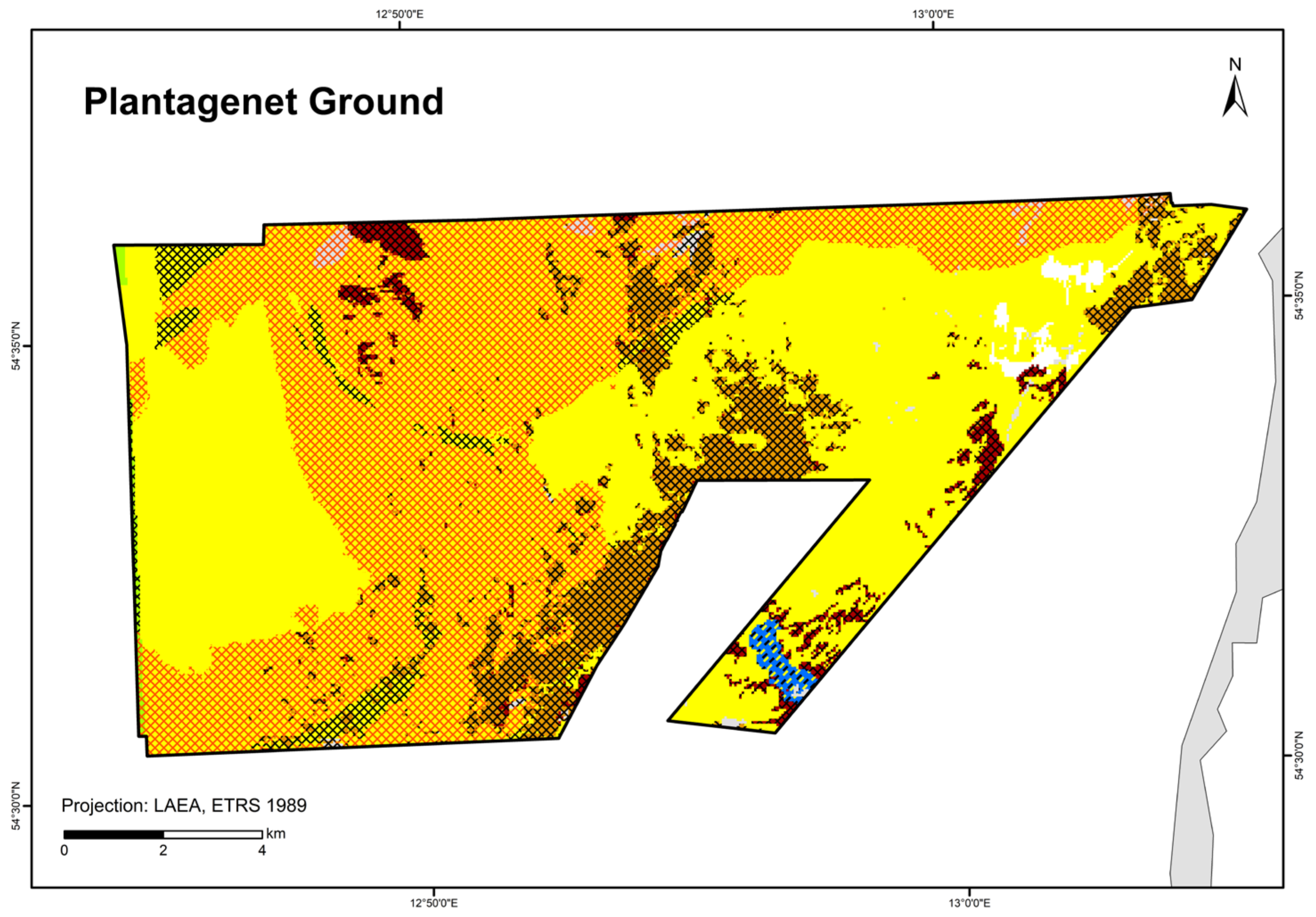
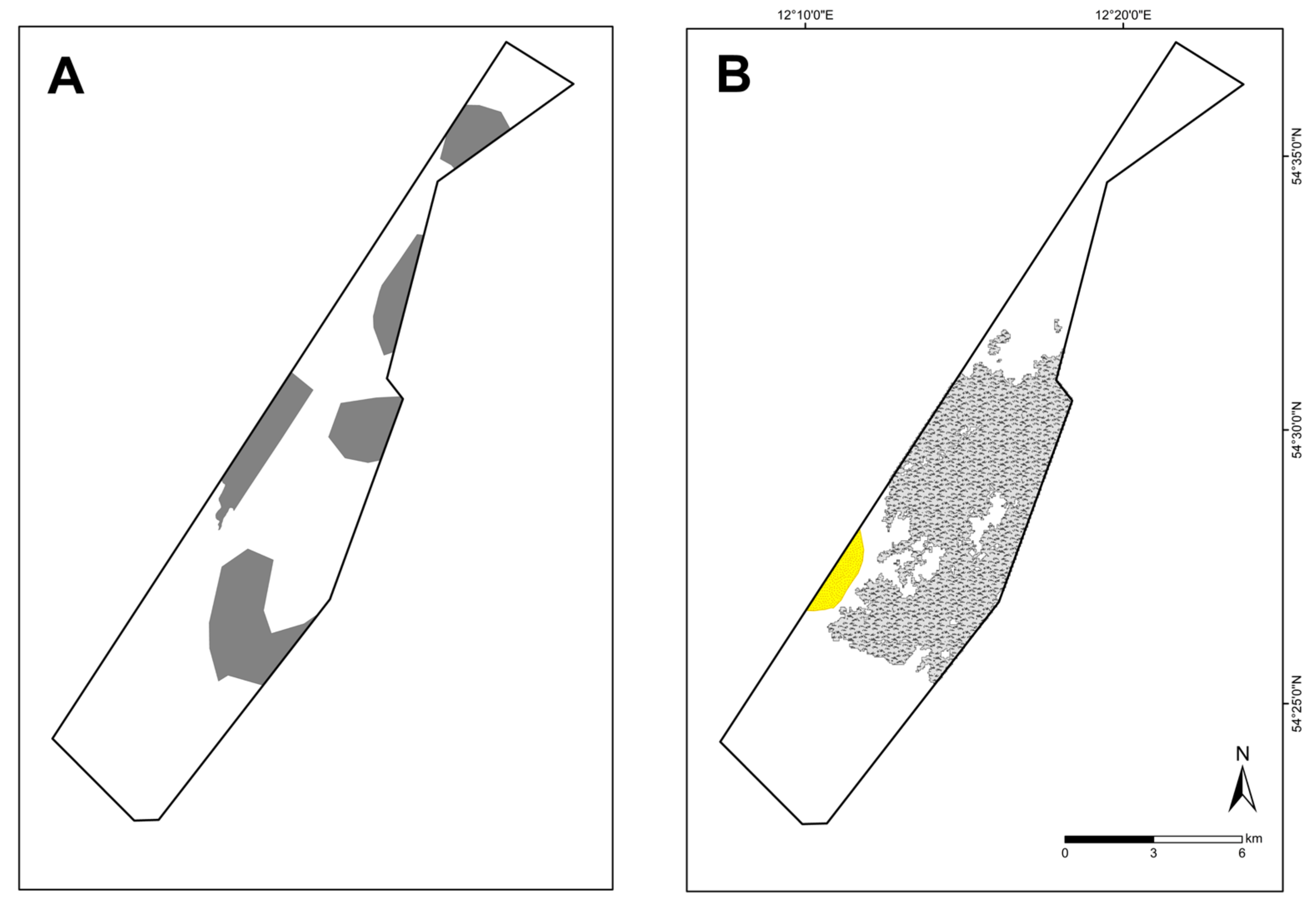
“Seagrass meadows and other marine macrophyte populations” (paragraph §30 Federal Nature Conservation Act)--Seagrass mapped in the “Plantagenet Ground”; other macrophytes modelled in this studyZostera spp. modelled in Schleswig-Holstein [40] and Mecklenburg-Western Pomerania [41]; Fucus spp. modelled in Schleswig-Holstein [40]; other macrophytes modelled in this studySee OHTSee OHT
Table 3. Translation of sediment types classified according to Tauber [32], following Folk [31] and Figge [36], into sediment classification according to EUNIS, on which the BHTs are based.
Sediment Type Classified according to Tauber (2012)Sediment Type Reclassified according to EUNIS
gravel, very coarse sandcoarse sediment
fine sand—coarse sandsand
very fine mud—very fine sandmud
clay, peat, lag sediment/tillmixed sediment (hard substrate)
Table 4. Number and sampling instruments of internal and external (in brackets) data that were mapped and acquired. Further data were obtained from the Federal Maritime and Hydrographic Agency (BSH), the State Office for the Environment, Nature Conservation and Geology of Mecklenburg-Western Pomerania (LUNG), the Schleswig-Holstein State Office for the Environment (LFU), the State Office for Agriculture and the Environment of Central Mecklenburg (StALU MM) and Western Mecklenburg (StALU WM), the Waterways and Shipping Office Stralsund (WSA Stralsund), the Christian-Albrechts-University Kiel (CAU Kiel), the Institute for Applied Ecosystem Research Ltd. (IfAÖ) (Neu Broderstorf, Germany), and the GEOMAR—Helmholtz Centre for Ocean Research Kiel.
AreaNumber of Acquired Data PointsSampling InstrumentsReferences of Used Data
Detail areasOuter Wismar Bay85 (18) grab stations, 29 video stations, 6 video transectsVan Veen grab, SeaViewer, BaSISIOW, IfAÖ, LUNG, StALU WM, StALU MM
Darss Sill73 (106) grab stations, 26 video stations, 4 video transectsVan Veen grab, SeaViewer, BaSISIOW, IfAÖ, LUNG, StALU WM, StALU MM
Plantagenet Ground49 (67) grab stations, 27 video stations, 4 video transectsVan Veen grab, SeaViewer, BaSISIOW, IfAÖ, LUNG, StALU WM, StALU MM
Kadet Trench103 (17) grab stations, 37 video stations, 8 video transects, 36 photo stationsVan Veen grab, SeaViewer, BaSIS, BfN drop cameraIOW, CAU Kiel, BSH
Fehmarn Belt339 grab stations, 134 video stations, 11 video transectsVan Veen grab, BaSISIOW, CAU Kiel, BSH
German Baltic Sea1637 (1991) grab stations, 403 video stations, 47 video transects, 59 photo stations, (45) diver stations, 9 (82) diver photo stationsVan Veen grab, SeaViewer, BaSIS, BfN drop camera, diver scratch samples and photosIOW, BfN, BSH, LFU, LUNG, StALU WM, StALU MM, WSA Stralsund, CAU Kiel, IfAÖ, Geomar
Table 5. Areas and their proportions of individual broad habitat types (BHT) in the German Baltic Sea.
BHTArea (km2)Area (%)
Infralittoral rock and biogenic reef1.00.007
Infralittoral mixed sediment (hard substrate)1785.311.6
Circalittoral mixed sediment (hard substrate)488.33.2
Infralittoral coarse sediment35.50.2
Circalittoral coarse sediment16.20.1
Infralittoral sand4600.029.8
Circalittoral sand3010.419.5
Infralittoral mud1393.89.0
Circalittoral mud4115.126.6
Table 6. Areas and their proportions of other individual habitat types (OHT) in the German Baltic Sea.
OHTArea (km2)Area within the German Baltic Sea (%)
Reefs (habitat type 1170)2183.514.1
Sandbanks (habitat type 1110)875.65.7
Seagrass meadows and other marine macrophyte populations321.42.1
Species-rich areas of gravel, coarse-sand, and shell-gravel areas5.90.04
Baltic aphotic muddy sediment dominated by ocean quahog (Arctica islandica)1417.69.2
Non-OHT10,641.668.9
Table 7. Mapped HELCOM HUB biotopes and their respective areas with colour indication, as shown in the HUB map (Figure 6). The question marks (?) represent unclassifiable sediment areas. Unclassifiable sediment areas, presumably representing lag sediment areas and/or mussel beds with or without glacial till, were labelled as “AA.I1E1?” (without boulders) or as “AA.M1E1?” (with boulders). The codes marked with an asterisk (*) were introduced in this study and do not yet exist in the HUB classification.
Colour Coding HUB MapHUB CodeHUB BiotopeArea (km2)
Biology 13 00006 i001AA.?Baltic photic benthos0.4
Biology 13 00006 i002AB.?Baltic aphotic benthos0.5
Biology 13 00006 i003AA.?1E1Baltic photic unknown substrate dominated by Mytilidae0.5
Biology 13 00006 i004AA.?3Baltic photic unknown substrate characterised by macroscopic infaunal biotic structures2.1
Biology 13 00006 i005AA.?3L3Baltic photic unknown substrate dominated by ocean quahog (Arctica islandica)0.003
Biology 13 00006 i006AB.?3L3Baltic aphotic unknown substrate dominated by ocean quahog (Arctica islandica)0.1
Biology 13 00006 i007AA.?3L4Baltic photic unknown substrate dominated by sand gaper (Mya arenaria)0.4
Biology 13 00006 i008AA.?3L9Baltic photic unknown substrate dominated by multiple infaunal bivalve species: Cerastoderma spp., Mya arenaria, Astarte borealis, Arctica islandica, Macoma balthica2.4
Biology 13 00006 i009AA.MBaltic photic mixed substrate0.02
Biology 13 00006 i010AB.MBaltic aphotic mixed substrate0.04
Biology 13 00006 i011AA.M1Baltic photic mixed substrate characterised by macroscopic epibenthic biotic structures14.4
Biology 13 00006 i012AB.M1Baltic aphotic mixed substrate characterised by macroscopic epibenthic biotic structures15.3
Biology 13 00006 i013AA.M1C1Baltic photic mixed substrate dominated by Fucus spp.102.8
Biology 13 00006 i014AA.M1C2Baltic photic mixed substrate dominated by perennial non-filamentous corticated red algae16.3
Biology 13 00006 i015AA.M1C3Baltic photic mixed substrate dominated by foliose red algae840.8
Biology 13 00006 i016AB.M1C3 *Baltic aphotic mixed substrate dominated by foliose red algae0.9
Biology 13 00006 i017AA.M1C5Baltic photic mixed substrate dominated by perennial filamentous algae24.2
Biology 13 00006 i018AA.M1E1Baltic photic mixed substrate dominated by Mytilidae540.6
Biology 13 00006 i019AA.M1E1?Baltic photic mixed substrate dominated by Mytilidae?0.2
Biology 13 00006 i020AB.M1E1Baltic aphotic mixed substrate dominated by Mytilidae302.9
Biology 13 00006 i021AA.M1G1Baltic photic mixed substrate dominated by hydroids (Hydrozoa)80.4
Biology 13 00006 i022AB.M1G1Baltic aphotic mixed substrate dominated by hydroids (Hydrozoa)109.0
Biology 13 00006 i023AA.M1H2Baltic photic mixed substrate dominated by erect moss animals (Flustra foliacea)0.02
Biology 13 00006 i024AB.M1I1Baltic aphotic mixed substrate dominated by barnacles (Balanidae)0.01
Biology 13 00006 i025AA.M1S1Baltic photic mixed substrate dominated by filamentous annual algae75.0
Biology 13 00006 i026AA.M1VBaltic photic mixed substrate characterised by mixed epibenthic macrocommunity0.1
Biology 13 00006 i027AB.M1VBaltic aphotic mixed substrate characterised by mixed epibenthic macrocommunity10.9
Biology 13 00006 i028AA.M2TBaltic photic mixed substrate characterised by sparse epibenthic macrocommunity36.0
Biology 13 00006 i029AB.M2TBaltic aphotic mixed substrate characterised by sparse epibenthic macrocommunity28.9
Biology 13 00006 i030AB.M4UBaltic aphotic mixed substrate characterised by no macrocommunity3.0
Biology 13 00006 i031AA.G+AA.J1E1Baltic photic peat bottoms + Baltic photic sand dominated by Mytilidae1.0
Biology 13 00006 i032AA.IBaltic photic coarse sediment0.006
Biology 13 00006 i033AA.I1E1Baltic photic coarse sediment dominated by Mytilidae11.4
Biology 13 00006 i034AA.I1E1?Baltic photic coarse sediment dominated by Mytilidae?0.7
Biology 13 00006 i035AB.I1E1Baltic aphotic coarse sediment dominated by Mytilidae9.0
Biology 13 00006 i036AA.I1C3Baltic photic coarse sediment dominated by foliose red algae0.1
Biology 13 00006 i037AA.I3Baltic photic coarse sediment characterised by macroscopic infaunal biotic structures10.5
Biology 13 00006 i038AB.I3Baltic aphotic coarse sediment characterised by macroscopic infaunal biotic structures3.9
Biology 13 00006 i039AA.I3L3 *Baltic photic coarse sediment dominated by ocean quahog (Arctica islandica)4.3
Biology 13 00006 i040AB.I3L3 *Baltic aphotic coarse sediment dominated by ocean quahog (Arctica islandica)2.0
Biology 13 00006 i041AA.I3L4 *Baltic photic coarse sediment dominated by sand gaper (Mya arenaria)0.2
Biology 13 00006 i042AA.I3L9 *Baltic photic coarse sediment dominated by multiple infaunal bivalve species: Cerastoderma spp., Mya arenaria, Astarte borealis, Arctica islandica, Macoma balthica4.1
Biology 13 00006 i043AB.I3L9 *Baltic aphotic coarse sediment dominated by multiple infaunal bivalve species: Cerastoderma spp., Mya arenaria, Astarte borealis, Arctica islandica, Macoma balthica1.7
Biology 13 00006 i044AA.I3L10Baltic photic coarse sediment dominated by multiple infaunal bivalve species: Macoma calcarea, Mya truncata, Astarte spp., Spisula spp.4.8
Biology 13 00006 i045AB.I3L10Baltic aphotic coarse sediment dominated by multiple infaunal bivalve species: Macoma calcarea, Mya truncata, Astarte spp., Spisula spp.1.0
Biology 13 00006 i046AA.I3L11Baltic photic coarse sediment dominated by multiple infaunal polychaete species including Ophelia spp.0.7
Biology 13 00006 i047AB.I3M6 *Baltic aphotic coarse sediment dominated by multiple infaunal polychaete species0.01
Biology 13 00006 i048AA.JBaltic photic sand0.1
Biology 13 00006 i049AB.JBaltic aphotic sand0.005
Biology 13 00006 i050AA.J1B7Baltic photic sand dominated by common eelgrass (Zostera marina)223.1
Biology 13 00006 i051AA.J1E1Baltic photic sand dominated by Mytilidae141.3
Biology 13 00006 i052AB.J1E1Baltic aphotic sand dominated by Mytilidae196.2
Biology 13 00006 i053AA.J1SBaltic photic sand characterised by annual algae4.0
Biology 13 00006 i054AA.J3Baltic photic sand characterised by macroscopic infaunal biotic structures425.9
Biology 13 00006 i055AB.J3Baltic aphotic sand characterised by macroscopic infaunal biotic structures121.5
Biology 13 00006 i056AA.J3L1Baltic photic sand dominated by Baltic tellin (Macoma balthica)8.2
Biology 13 00006 i057AB.J3L1Baltic aphotic sand dominated by Baltic tellin (Macoma balthica)60.7
Biology 13 00006 i058AA.J3L3Baltic photic sand dominated by ocean quahog (Arctica islandica)367.4
Biology 13 00006 i059AB.J3L3Baltic aphotic sand dominated by ocean quahog (Arctica islandica)252.4
Biology 13 00006 i060AA.J3L4Baltic photic sand dominated by sand gaper (Mya arenaria)15.7
Biology 13 00006 i061AB.J3L4Baltic aphotic sand dominated by sand gaper (Mya arenaria)0.1
Biology 13 00006 i062AA.J3L9Baltic photic sand dominated by multiple infaunal bivalve species: Cerastoderma spp., Mya arenaria, Astarte borealis, Arctica islandica, Macoma balthica2338.7
Biology 13 00006 i063AB.J3L9Baltic aphotic sand dominated by multiple infaunal bivalve species: Cerastoderma spp., Mya arenaria, Astarte borealis, Arctica islandica, Macoma balthica2381.1
Biology 13 00006 i064AA.J3L10Baltic photic sand dominated by multiple infaunal bivalve species: Macoma calcarea, Mya truncata, Astarte spp., Spisula spp.1.1
Biology 13 00006 i065AB.J3L10Baltic aphotic sand dominated by multiple infaunal bivalve species: Macoma calcarea, Mya truncata, Astarte spp., Spisula spp.1.2
Biology 13 00006 i066AA.J3L11Baltic photic sand dominated by multiple infaunal polychaete species including Ophelia spp.5.7
Biology 13 00006 i067AA.J3M6*Baltic photic sand dominated by multiple infaunal polychaete species0.005
Biology 13 00006 i068AB.J3M6*Baltic aphotic sand dominated by multiple infaunal polychaete species0.3
Biology 13 00006 i069AA.H1B7Baltic photic muddy sediment dominated by common eelgrass (Zostera marina)69.0
Biology 13 00006 i070AA.H1E1Baltic photic muddy sediment dominated by Mytilidae46.6
Biology 13 00006 i071AB.H1E1Baltic aphotic muddy sediment dominated by Mytilidae15.0
Biology 13 00006 i072AA.H1SBaltic photic muddy sediment characterised by annual algae1.0
Biology 13 00006 i073AA.H3Baltic photic muddy sediment characterised by macroscopic infaunal biotic structures65.2
Biology 13 00006 i074AB.H3Baltic aphotic muddy sediment characterised by macroscopic infaunal biotic structures546.4
Biology 13 00006 i075AB.H3L1Baltic aphotic muddy sediment dominated by Baltic tellin (Macoma balthica)1131.6
Biology 13 00006 i076AA.H3L3Baltic photic muddy sediment dominated by ocean quahog (Arctica islandica)249.9
Biology 13 00006 i077AB.H3L3Baltic aphotic muddy sediment dominated by ocean quahog (Arctica islandica)1435.5
Biology 13 00006 i078AA.H3L4 *Baltic photic muddy sediment dominated by sand gaper (Mya arenaria)0.003
Biology 13 00006 i079AB.H3L4 *Baltic aphotic muddy sediment dominated by sand gaper (Mya arenaria)0.005
Biology 13 00006 i080AA.H3L9 *Baltic photic muddy sediment dominated by multiple infaunal bivalve species: Cerastoderma spp., Mya arenaria, Astarte borealis, Arctica islandica, Macoma balthica307.9
Biology 13 00006 i081AB.H3L9 *Baltic aphotic muddy sediment dominated by multiple infaunal bivalve species: Cerastoderma spp., Mya arenaria, Astarte borealis, Arctica islandica, Macoma balthica991.0
Biology 13 00006 i082AA.H3L10 *Baltic photic muddy sediment dominated by multiple infaunal bivalve species: Macoma calcarea, Mya truncata, Astarte spp., Spisula spp.0.003
Biology 13 00006 i083AB.H3L10 *Baltic aphotic muddy sediment dominated by multiple infaunal bivalve species: Macoma calcarea, Mya truncata, Astarte spp., Spisula spp.0.1
Biology 13 00006 i084AB.H3M6Baltic aphotic muddy sediment dominated by multiple infaunal polychaete species3.2
NA8.0
Table 8. Overall performance of the selected model in the respective detail areas and the German Baltic Sea; 95% CI: 95 % confidence interval of overall accuracy, AUC: area under (receiver operating characteristic) curve. Epibenthic communities did not need to be modelled in the “Plantagenet Ground”, as only mussels dominated the hard bottoms in this eastern area.
EndobenthosEpibenthos
AreaOverall Accuracy95% CIAUCKappaMost Important VariablesOverall Accuracy95% CIAUCKappaMost Important Variables
Detail areasOuter Wismar Bay0.3930.215–0.5940.7580.035current velocity
(10th percentile)
0.980.893–10.9750.96DOC (10th percentile), O2 (10th percentile)
Darss Sill0.5640.423–0.70.6480.453temperature
(10th percentile)
10.936–111DOC (mean)
Plantagenet Ground0.7190.533–0.8630.7970.559sedimentNANANANANA
Kadet Trench0.7590.565–0.90.7860.576shear stress (mean), current velocity N/S
(90 percentile)
0.6570.556–0.7480.7160.485depth
Fehmarn Belt0.763NA0.7880.563sediment, depth0.926NA0.9150.83DOC (mean), depth
German Baltic Sea0.6660.636–0.6950.7040.535sediment0.7970.770–0.8210.8050.712depth, salinity (mean)
Disclaimer/Publisher’s Note: The statements, opinions and data contained in all publications are solely those of the individual author(s) and contributor(s) and not of MDPI and/or the editor(s). MDPI and/or the editor(s) disclaim responsibility for any injury to people or property resulting from any ideas, methods, instructions or products referred to in the content.

