Closed-Form Solution Procedure for Simulating Debonding in FRP Strips Glued to a Generic Substrate Material

Abstract

The present paper proposes a useful closed-form solution for a wide class of mechanical problems, among which one of the most relevant and debated is the deboning process of Fiber-Reinforced Polymer (FRP) strips glued to generic materials and possibly intended as a mode-II fracture process. Specifically, after outlining well-known equations, a novel piecewise analytical formulation based on a cascading solution process is proposed with the aim of keeping the mathematical expressions of the relevant mechanical quantities as simple as possible. Although other analytical solutions and numerical procedures are already available in the literature, the present one is capable of handling the softening or snap-back response deriving from the full-range simulation of the depending process with no need for complex numerical techniques. This is obtained by considering the slip at the free end of the strip as the main displacement control parameter. After some comparisons between the proposed closed-form solution and experimental results available in the literature, some mechanical considerations are highlighted by elaborating on the results of a parametric study considering the variation of the main geometric and mechanical quantities. The numerical code implemented as part of the present study is available to readers in Open Access.

1. Introduction

Fiber-Reinforced Polymer (FRP) systems are well-established nowadays among the possible technical solutions available on the market for strengthening structural members in existing civil engineering constructions [1]. Although the first applications of FRP strengthening were on reinforced concrete (RC) members [2], composite systems are also widely adopted for masonry structures [3], and, more recently, their usage is becoming more and more common also with steel [4] and timber [5] constructions.

Codes and guidelines have been recently released [6] (or are currently in a preliminary version [7,8]) with the aim of making the FRP strengthening of existing structure safe and reliable.

However, several issues still need further investigation with the aim of advancing engineers’ understanding of the mechanical behavior of FRP-strengthened structural members [9]. Among them, the adhesion between FRP and the existing material substrate deserves special attention, as debonding [10] often controls the mechanical response of FRP-strengthened members [11] and their failure mode [12].

Several models have been proposed with the aim of simulating the full-range behavior of FRP-strengthened members [13,14]; they often assume that debonding develops as pure mode-II fracture propagation process. In other words, they are based on assuming an interface interaction law between relative axial displacements (often referred to as “interface slips”) and the corresponding shear bond stresses; conversely, possible relative displacements in the normal direction of the interface (“uplifts”) are neglected, and the corresponding normal stresses not considered in defining debonding conditions.

The assumptions briefly recalled above, yet significantly simplified, require the detailed definition of a bond-slip law controlling the adhesive interaction between the FRP strips and the material substrate throughout the whole interface. Therefore, with specific reference to the case of the so-called Externally Bonded (EB) FRP strengthening of structures, several proposals are available in the literature to define the aforementioned bond-slip laws [15], though the most widely employed is the well-known bilinear elastic-softening relationship.

The relevant parameters of bond-slip laws can be identified by processing the results of pull-out tests on FRP strips glued on the substrate material of interest for the application under consideration. In fact, several results obtained from pull-out tests executed on FRP strips bonded on concrete blocks are available in the scientific literature, more with reference of monotonic tests [16], but also considering cyclic loading protocols [17].

In fact, experimental results from pull-out tests does not allow one to “directly” determine the mechanical parameters needed to identify the bond-slip laws, as the latter are based on the interaction between FRP strip and the substrate material that, in principle, cannot be “measured” by means of experimental tests. Conversely, “inverse” (or “indirect”) identification methods are needed to process the results of pull-out tests and obtain the relevant parameters of the bond-slip law that can reduce the differences between the experimentally observed response and the results of a simulation based on the assumption of the bond-slip law under consideration [18].

Inverse identification procedures are based upon theoretical models (and their analytical or numerical solutions) that are employed to simulate the mechanical response of the structural system under consideration (namely, a FRP-to-concrete joint subjected to a pull-out test) with the aim of quantifying the difference between the simulated and experimental results and of reducing them (through automated constrained optimization procedures) by looking for the “best” values for the material parameters; in the case under consideration, the latter are the mechanical quantities describing bond-slip laws [18].

Therefore, the availability of accurate and efficient models capable of simulating the mechanical response of FRP-to-concrete (or other supporting materials) joints subjected to pull-out actions is an essential point to obtain unbiased predictions (characterized by low epistemic uncertainties) and reasonably fast inverse identification procedures. Numerical solutions based on time-consuming iterative/incremental numerical methods are, then, unfit to be employed in inverse identification processes that, in principle, may require several runs during the optimization process. Hence, when possible, analytical solutions are certainly preferable to this aim, as they can be both accurate (as far as the assumption which they are based on are consistent) and fast (because they do not require significantly iterative calculations).

In the case of the bilinear elastic-softening bond-slip law, the one actually considered in the present study, a first and incomplete piecewise analytical solution has been proposed by the author, but it has had limited circulation in the scientific community because it was only included in a book of a conference proceeding [19]. In the following years, various authors came up with alternative solution strategies, mainly limited to the case of “long” anchorage length of the FRP plate on the supporting material [20]; other solutions were aimed at simulating the stress and strain distributions developing between two subsequent cracks in FRP-strengthened RC beams in bending [21].

This paper presents a further evolution of a “fully analytical” solution developed in a previously co-authored paper [22]. The novelty of the present work is twofold. On the one hand, the proposed closed-form formulation is based on a cascading solution of the differential equation, which makes the resulting analytical expressions more handy and simpler. On the other hand, a Matlab code implementing the whole solution process is provided in Open Access as Supplementary Materials, which makes the present solution fully accessible to readers, especially to those (e.g., young researchers) who are approaching the topic for the first time.

The paper recalls the main mechanical assumptions and presents the analytical solutions derived for the various stages of the debonding process (Section 2). Then, some comparisons with available experimental results are proposed (Section 3), and the outcome of some theoretical analyses are shown with the aim to point out the role of the various geometric and mechanical parameters on the resulting debonding process (Section 4). Final considerations are mentioned in Section 5.

2. Model Formulation

2.1. Mechanical Assumptions

The mechanical model proposed herein to simulate the mechanical response of FRP strips glued to a generic material is based on the following main assumptions:

-

Debonding develops in pure mode II, and hence only relative slips are relevant to describing the displacement field of the FRP strip;

-

The FRP strip responds elastically with a Young modulus E_f;

-

Interface slips are uniform throughout the generic transversal chord of the FRP strip;

-

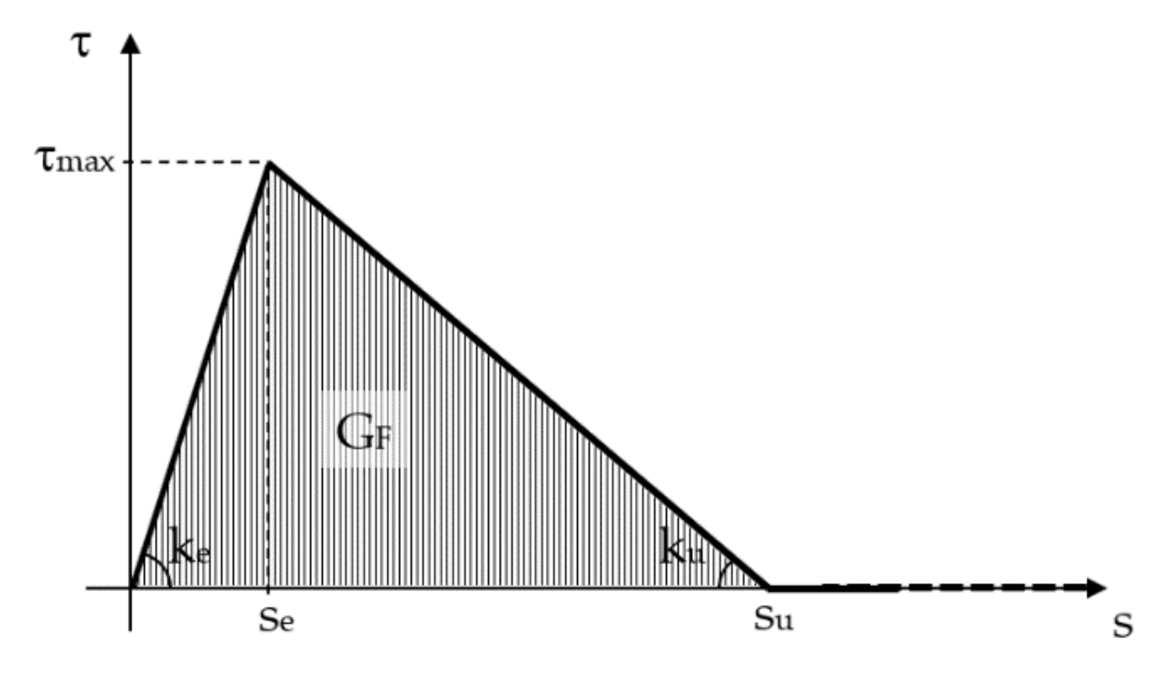
The interface is described by a bilinear elastic-softening bond-slip law;

-

The substrate material is supposed to be stiff.

The assumed bond-slip law (Figure 1) is defined by three parameters, namely, the slip s_el at the end of the elastic branch, the slip s_u at the end of the softening branch, and the maximum bond shear stress τ_max. Related properties are the stiffnesses k_e = τ_max/s_e and k_u = τ_max/(s_u − s_e) of the two linear branches and the specific fracture energy G_F = τ_max s_u/2.

Thus, the analytical expressions of the bond-slip law can be written as follows:

$$\tau \left(s\right)=\left\{\begin{array}{lll}{k}_{e}s\hfill & if\hfill & s\le s_e\hfill \\ {\tau }_{\max }-k_u\left(s-s_e\right)\hfill & if\hfill & s_e<s\le s_u.\hfill \\ 0\hfill & if\hfill & s>s_u\hfill \end{array}\right.$$

(1)

2.2. Main Equations and Close-Form Solutions

Imposing equilibrium conditions (between axial stresses σ and interface bond stresses τ) and compatibility conditions (between slip s and axial strains ε in the FRP strip) on a segmental strip element (Figure 2) leads to the two following differential equations:

$$\frac{d\sigma }{dz}-\frac{\tau \left(s\right)}{t_f}=0$$

(2)

$$\frac{ds}{dz}=\epsilon \Rightarrow \frac{ds}{dz}=\frac{\sigma }{E_f}$$

(3)

which, in turn, lead to the well-known differential equations reported below [22]:

$$\frac{d^{2}s}{d{z}^2}-\frac{\tau \left(s\right)}{E_f{t}_f}=0$$

(4)

where t_f is the thickness, respectively, of the FRP plate.

Equation (4) assumes three different expressions depending on the one taken by the bond slip law τ(s), which depends on whether the slip s falls within the elastic, softening or debonded branch, as described by the three terms on the right-end side of Equation (1).

Replacing each one of such expressions in Equation (4), the latter leads to the three following elementary closed-form general integrals reported hereafter:

-

Elastic (“El”) branch (s ≤ s_e):

$$s_{El}\left(z\right)=A_{El}\cosh \left({\alpha }_{e}z\right)+B_{El}\sinh \left({\alpha }_{e}z\right)\hspace{1em}\hspace{1em}\hspace{1em}\mathrm{with}\hspace{1em}\hspace{1em}\hspace{1em}{\alpha }_e{}^2=\frac{k_e}{E_f{t}_f}$$

(5)

-

Softening (“So”) branch (s_e < s ≤s_u):

$$s_{So}\left(z\right)=A_{So}\cos \left({\alpha }_{u}z\right)+B_{So}\sinh \left({\alpha }_{u}z\right)+s_u\hspace{1em}\hspace{1em}\hspace{1em}\mathrm{with}\hspace{1em}\hspace{1em}\hspace{1em}{\alpha }_u{}^2=\frac{k_u}{E_f{t}_f};$$

(6)

-

Debonded (“De”) branch (s > s_u):

$$s_{De}\left(z\right)=A_{De}+B_{De}z.$$

(7)

Details about the mathematical derivations of the expressions in Equations (5)–(7) are omitted herein for the sake of brevity and can be found in a previous work [22].

2.3. Piecewise Formulation for Simulating the Debonding Process

The following subsections propose piecewise closed-form solutions for the debonding process up to failure.

2.3.1. Elastic (“El”) Stage

As long as interface slips s are smaller than s_e, the elastic solution of Equation (5) completely describes the distribution of slips throughout the whole bond length L, the adhesive interface being in the elastic branch. Therefore, after imposing the following initial conditions (namely, a slip s₀ and zero axial strain at the unloaded end):

$$\left\{\begin{array}{l}{s}_{El}(z=0)=s_0\hfill \\ {\left.\frac{d{s}_{El}}{dz}\right|}_{z=0}=0\hfill \end{array}\right.$$

(8)

the following solutions can be found in terms of displacement distribution:

$$s_{El}(z)=\cosh \left(\alpha z\right)\cdot s_0$$

(9)

which leads to the slip s_L,El at the end of the bond length and the applied force F_El determined as follows:

$$s_{L,El}=s_{El}(z=L)=\cosh \left(\alpha L\right)\cdot s_0$$

(10)

$$F_{El}=E_f{b}_f{t}_f\cdot {\left.\frac{d{s}_{El}}{dz}\right|}_{z=L}=E_f{b}_f{t}_f\cdot \alpha s_0\sinh \left(\alpha L\right).$$

(11)

Therefore, Equation (11) represents the applied force corresponding to imposed slips (at the end of the bonded length, namely at z = L). Moreover, the end of the elastic branch is achieved as soon as s_L,El ≤ s_e, which, from Equation (10), leads to the following limitation in terms of imposed slip s₀ at the unloaded end:

$$s_0\le s_{0,El}=\mathrm{sech}\left(\alpha L\right)\cdot s_e.$$

(12)

2.3.2. Elastic-Softening (“El-So”) Stage

As the slip s_L at the loaded end of the bond length becomes higher than s_e, a part of the bonded interface attains the softening branch of the bond-slip law described by Equation (1). A piecewise “cascading” solution scheme can be followed with the aim to reduce the analytical effort needed to obtain the closed-form expressions of the slip distributions throughout the two parts of the interface responding in the elastic and softening branch, respectively.

Starting from values of s₀ higher than those limited by the Equation (12), the slip distribution throughout the elastic part of the interface can still be obtained by means of s_El in expression (9), which, indeed, is admissible as long as s_El(z) ≤ s_e. Hence, solving the equation defined by imposing the right end side of expression (9) be equal to s_e, the following limit abscissa for the elastic part of the interface:

$$\overline{z}=\frac{1}{\alpha }\cdot \ln \left[\frac{s_e}{s_0}\cdot \left(1-\sqrt{1-{\left(\frac{s_0}{s_e}\right)}^2}\right)\right],$$

(13)

which, in principle, ranges from L, when s₀ = s_0,El of Equation (12), and back to 0, when s₀ = s_e.

According to the novel “cascading” solution procedure, the expression of slips where s_e < s ≤ s_u can be determined by coupling the general integral of Equation (6) with the following initial conditions:

$$\left\{\begin{array}{l}{s}_{So}(z=\overline{z})=s_e\hfill \\ {\left.\frac{d{s}_{So}}{dz}\right|}_{z=\overline{z}}={\left.\frac{d{s}_{El}}{dz}\right|}_{z=\overline{z}}\hfill \end{array}\right..$$

(14)

After simple mathematical elaborations, the following expression can be obtained for slips in the part of the interface stressed in the softening branch of the bond-slip law:

$$s_{So}\left(z\right)=s_u-\left(s_u-s_e\right)\cdot \cos \left[\beta \left(z-\overline{z}\right)\right]+\frac{\alpha s_e\cdot \sin \left[\beta \left(z-\overline{z}\right)\right]\cdot \tanh \left(\alpha \overline{z}\right)}{\beta }$$

(15)

which leads to the following expressions for the slip s_L,El-So at the end of the bond length and the corresponding applied force F_El-So:

$$s_{L,El\text{-}So}=s_{So}(z=L)=s_u-\left(s_u-s_e\right)\cdot \cos \left[\beta \left(L-\overline{z}\right)\right]+\frac{\alpha s_e\cdot \sin \left[\beta \left(L-\overline{z}\right)\right]\cdot \tanh \left(\alpha \overline{z}\right)}{\beta }$$

(16)

$$\begin{array}{l}{F}_{El-So}=E_f{b}_f{t}_f\cdot {\left.\frac{d{s}_{So}}{dz}\right|}_{z=L}=\\ =E_f{b}_f{t}_f\cdot \left\{\alpha \cdot s_e\cdot \cos \left[\beta \cdot \left(L-\overline{z}\right)\right]\cdot \tanh \left(\alpha \overline{z}\right)+\beta \cdot \left(s_u-s_e\right)\cdot \sin \left[\beta \cdot \left(L-\overline{z}\right)\right]\right\}\end{array}$$

(17)

Therefore, the solution is controlled by the value of s₀ imposed at the free end, which, in turn, controls the value of $\overline{z}$ through Equation (13), and hence the values of slips and force at the end of the bonded length L of the FRP strip.

2.3.3. Definition of “Short” and “Long” Anchorage

The El-So stage lasts up to either the slip s₀ at the free end (z = 0) achieves s_e or the slip s_L (at s = L) attains s_u. The first condition can easily be checked, as s₀ is actually the imposed displacement. Conversely, the second condition (s_L = s_u), imposed to the s_L,El-So expression (16) of the s_L slip, leads to the following mathematical condition:

$$s_{L,El\text{-}So}=s_u\Rightarrow \beta \left(s_u-s_e\right)\cdot \cos \left[\beta \left(L-\overline{z}\right)\right]=\alpha s_e\cdot \sin \left[\beta \left(L-\overline{z}\right)\right]\cdot \tanh \left(\alpha \overline{z}\right).$$

(18)

After some mathematical transformations, also including the identity between the α, β, s_e and s_u − s_e that can be derived by combining the definitions of α² and β² in Equations (5) and (6), the following relationship can be stated to determine the value of $\overline{z}$ (and hence of s₀) leading to s_L = s_u:

$$\alpha \cdot \cot \left[\beta \left(L-\overline{z}\right)\right]=\beta \cdot \tanh \left(\alpha \overline{z}\right).$$

(19)

Equation (19) has two main implications. The first one has to do with its solution in terms of $\overline{z}$; although no analytical solutions are available for this transcendental equation, a reasonable approximation can be obtained by assuming that the hyperbolic tangent function at the right-end side tends to 1, which would lead to the following relationship:

$${\overline{z}}_{El\text{-}So}\approx L-\frac{1}{\beta }\cdot \arctan \left[\left(\frac{\alpha }{\beta }\right)\right].$$

(20)

The second one defines the limit condition of having both s₀ = s_e (namely, $\overline{z}=0$) and s_L = s_u, which leads to the following relationship between the length L and the values of β:

$$\alpha \cdot \cot \left[\beta \left(L\right)\right]=0\Rightarrow \overline{L}=\frac{\pi }{2\beta }$$

(21)

where the $\overline{L}$ represents a critical value for the bond length L. More specifically:

-

for $L<\overline{L}$ (“short” anchorage), the condition s₀ = s_e at the free end is attained, while s_L < s_u: therefore, the debonding process proceeds towards a situation in which s_e < s(z) < s_u, meaning that the whole interface is stressed in the softening branch (“So” stage) of the bond-slip relationship (1);

-

for $L\ge \overline{L}$ (“long” anchorage), the condition s_L = s_u is attained, while s₀ < s_e; therefore, the debonding process proceeds towards a situation in which the interface can be subdivided into three regions (“El-So-De”): the first one [0,$\overline{z}$] reacts elastically, the second one ($\overline{z}$,$\overline{\overline{z}}$] mobilizes bond stresses in the softening branch, and the third one ($\overline{\overline{z}}$,L] is debonded.

2.3.4. Short Anchorage: Debonding Evolution to Failure (“So” Stage)

The slip distribution of the so-called “So” stage can be obtained by coupling the general integral (6) with the following initial conditions:

$$\left\{\begin{array}{l}{s}_{So}(z=0)=s_0>s_e\hfill \\ {\left.\frac{d{s}_{So}}{dz}\right|}_{z=0}=0\hfill \end{array}\right.$$

(22)

which leads to the following solution:

$$s_{So}(z)=s_u-\left(s_u-s_0\right)\cdot \cos \left(\beta z\right).$$

(23)

In this condition, the following expressions can be determined for both the slip s_L,So at the end of the bond length and the correspondingly applied force F_So:

$$s_{L,So}=s_{So}(z=L)=s_u-\left(s_u-s_0\right)\cdot \cos \left(\beta L\right)$$

(24)

$$F_{So}=E_f{b}_f{t}_f\cdot {\left.\frac{d{s}_{So}}{dz}\right|}_{z=L}=\beta \cdot \left(s_u-s_0\right)\cdot E_f{b}_f{t}_f\cdot \sin \left(\beta L\right).$$

(25)

It is apparent that, as s₀ tends to s_u (in which case the FRP strip is fully debonded) the value of s_L,So also tends to s_u and the force F_So vanishes.

2.3.5. Long Anchorage: Debonding Evolution to Failure (“El-So-De” Stage)

The slip distribution of the so-called “El-So-De” is obtained by combining the elastic solution (9) for z ∈ [0,$\overline{z}$], the softening (15) for z ∈ ($\overline{z}$,$\overline{\overline{z}}$], and a final “piece” based on the general integral (7).

First, the expression of $\overline{\overline{z}}$ can be determined by equaling s_So(z) defined by Equation (15) to s_u; the expression reported hereafter can be obtained after some mathematical simplifications:

$$\overline{\overline{z}}=\overline{z}+\frac{1}{\beta }\cdot \arctan \left[\frac{\alpha }{\beta \cdot \tanh \left(\alpha \overline{z}\right)}\right].$$

(26)

It is worth highlighting that the combination of Equations (19) and (26) guarantees that $\overline{\overline{z}}<L$.

Then, the slip distribution throughout the debonded part of the interface z ∈ ($\overline{\overline{z}}$,L] can be obtained, again according to the “cascading” process followed in other stages, by coupling the general integral (7) with the following initial conditions:

$$\left\{\begin{array}{l}{s}_{De}(z=\overline{\overline{z}})=s_u\hfill \\ {\left.\frac{d{s}_{De}}{dz}\right|}_{z=\overline{\overline{z}}}={\left.\frac{d{s}_{So}}{dz}\right|}_{z=\overline{\overline{z}}}\hfill \end{array}\right.$$

(27)

which leads to the following solution:

$$s_{De}(z)={\overline{A}}_{De}+{\overline{B}}_{De}\cdot z$$

(28)

with

$${\overline{B}}_{De}=\beta \left(s_u-s_e\right)\sin \left[\beta (\overline{\overline{z}}-\overline{z})\right]+\alpha s_e\cos \left[\beta (\overline{\overline{z}}-\overline{z})\right]*\tanh \left(\alpha \overline{z}\right)$$

(29)

$${\overline{A}}_{De}=su-{\overline{B}}_{De}\cdot \overline{\overline{z}}.$$

(30)

The process is always controlled by the slip s₀ imposed at the free end, which defines both $\overline{z}$ through the solution of Equation (19) (possibly approximate by the expression (20)) and $\overline{\overline{z}}$ through expression (26). The “El-So-De” stage lasts up until the imposed slip at the free end achieves s_e; then the full debonding is achieved by means of a stress regime that resembles the “So” stage with $L=\overline{L}$, the remaining $L-\overline{L}$ length being already debonded. As in the case of Equations (24) and (25), the force-slip relationship is linear up to full debonding (s = s_u) and debonding (F = 0). The analytical details of this stage are omitted for the sake of brevity.

2.3.6. Final Considerations about the Simulation of the Debonding Process

The previous subsections have clearly formulated a closed form piecewise formulation of the debonding phenomenon in FRP strips bonded to a quasi-brittle substrate. The main novelty with respect to a previous formulation [22] is represented by the fact that the main control parameter is the displacement at the free end s₀ (whereas the former was based on s_L) and a “cascading” solution process involving subsets of maximum two equations, which leads to simpler expressions. Under a mathematical standpoint, the present formulation is based on the solution of a series initial value problems (in space), whereas the former was based on a unique boundary value problem for each stage of the debonding process.

Finally, it is worth highlighting that the relationships reported in the previous subsections allow determining both the global s_L-F relationship and the interface slip s(z) distribution for the generic stage of the debonding process controlled by a value of the free end slip s₀ ranging from 0 to s_u. It goes without saying that, according to the compatibility condition (3), the distribution of axial strains ε(z) can be determined as the first derivative of s(z) with respect to the abscissa z; similarly, the distribution of interface bond stresses τ(z) can be determined by converting the interface slip s(z) via the bond-slip law (1).

3. Experimental Comparisons

This section proposes some comparisons between the experimental results available in the literature and the results of simulations obtained by running an analysis based on the proposed closed-form solution. Specifically, two sets of well-known experimental results are considered hereafter.

The first one comes from a highly cited experimental study reporting the results of four nominally equal specimens that are only different in terms of bonded length, the latter ranging between 2 and 8 inches [16]. The second one is taken from a very recent experimental study [17] consisting, among other things, of monotonic pull-out tests on three nominally equal specimens with properties significantly different with respect to the previous one.

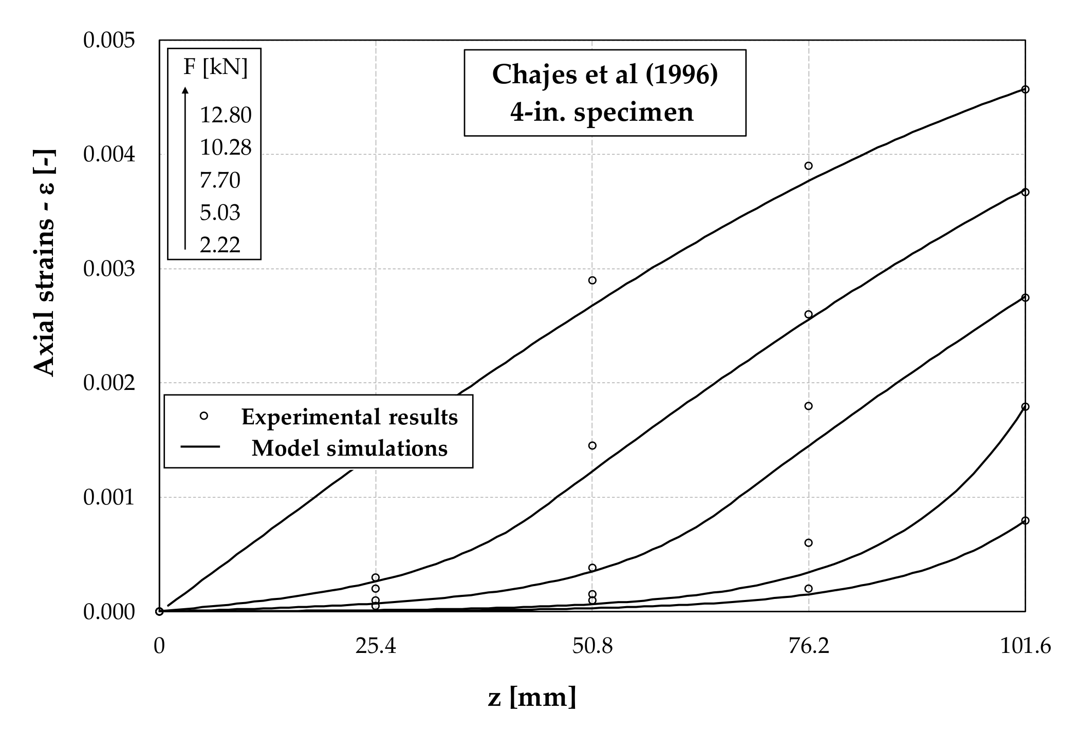
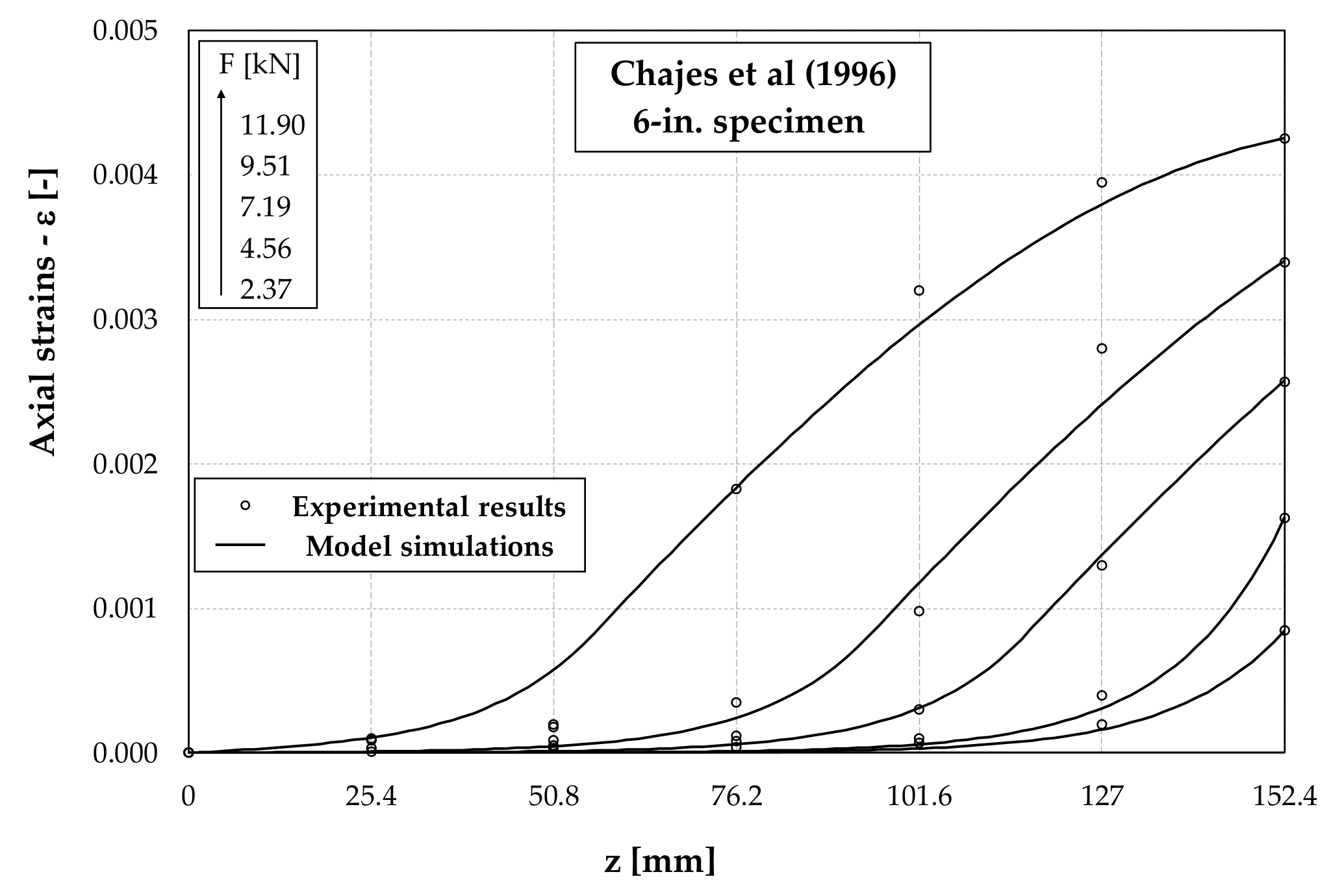
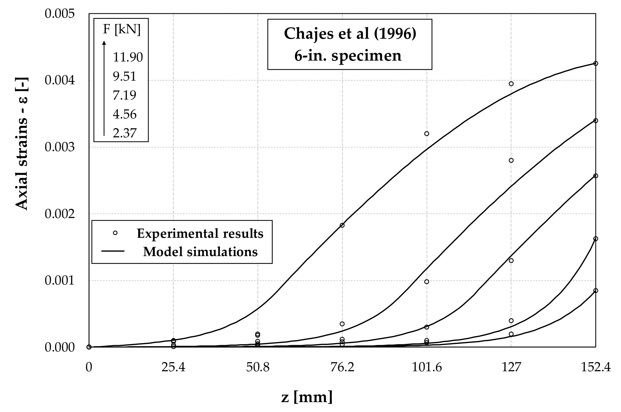
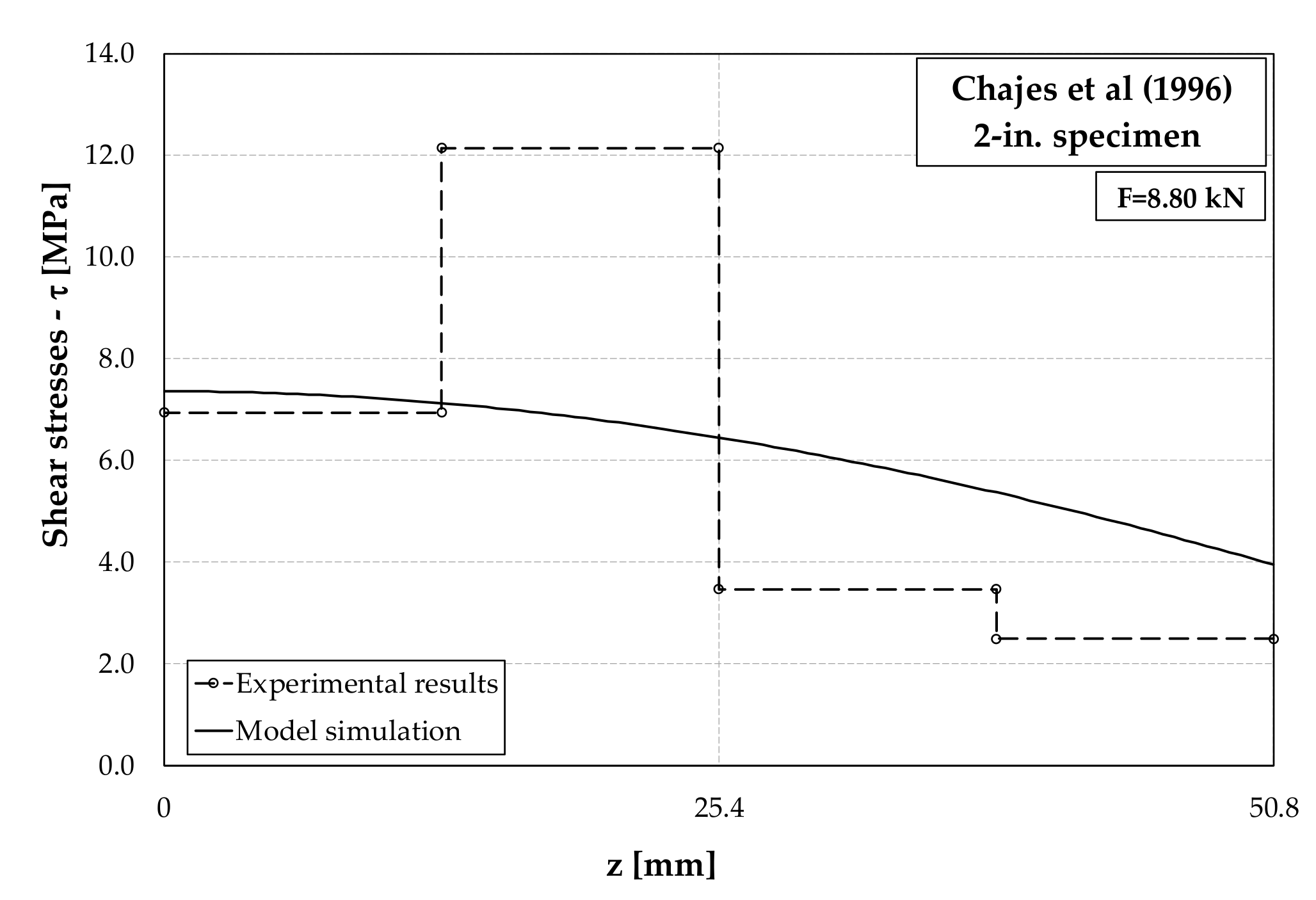
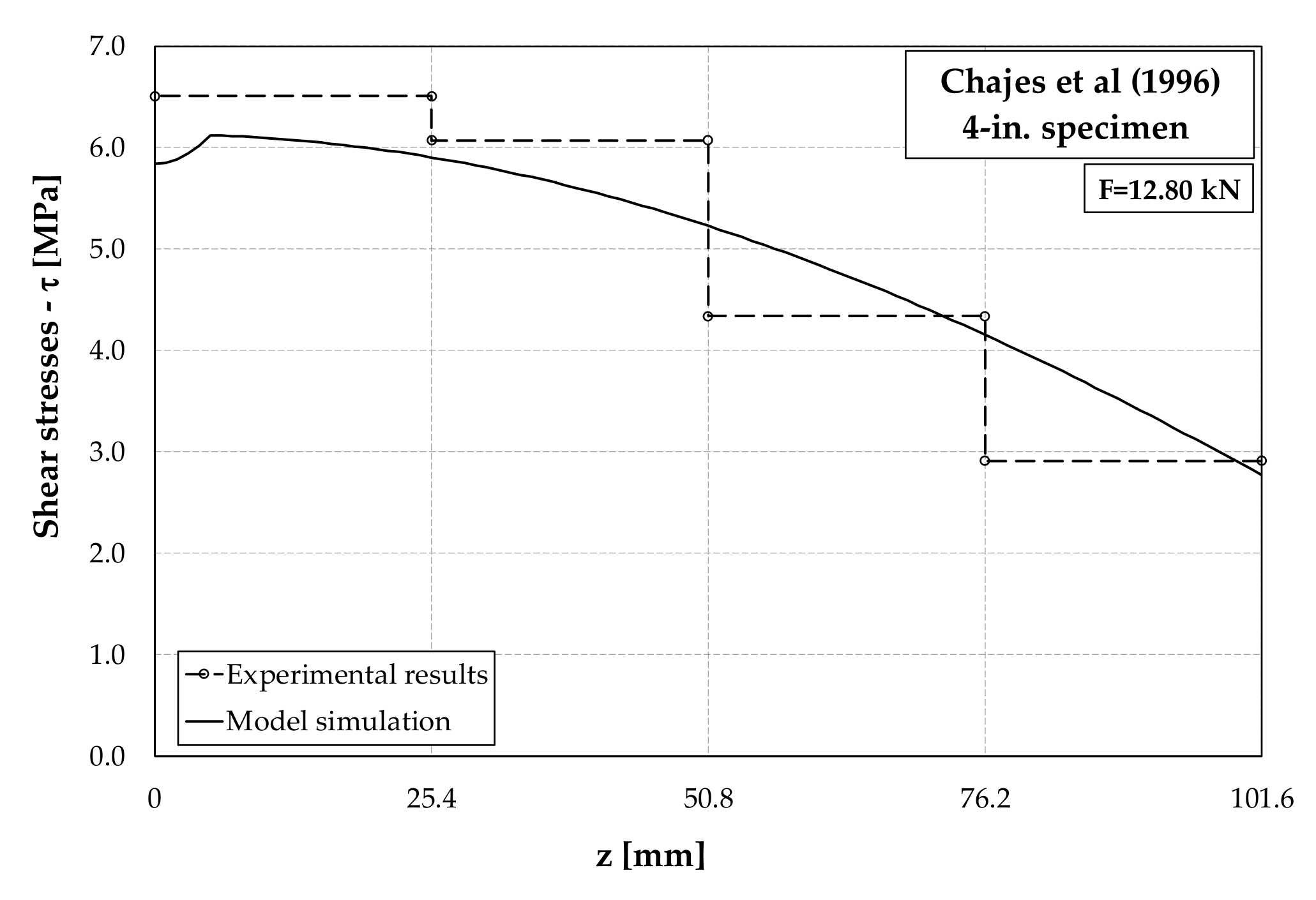
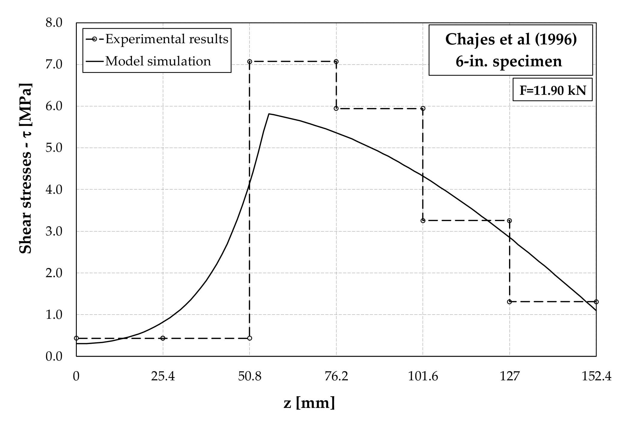
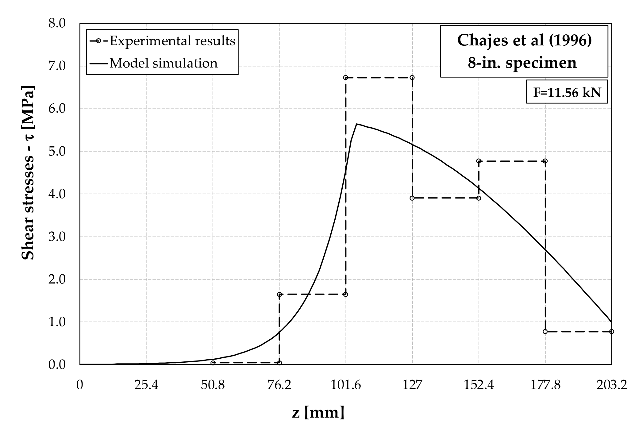
3.1. Pull-Out Tests by Chajes et al. (1996)

The results of four single-side pull-out tests with various bond lengths, including both cases of “short” and “long” anchorage as defined in Section 2.3.3, are considered in the following with the aim to compare the experimentally measured values of axial strains recorded at different load levels with the corresponding predictions deriving from the proposed model. Specifically, bond lengths of 2, 4, 6, and 8 inches (corresponding to 50.8, 101.6, 152.4, 203.2 mm) are considered for a strip of carbon FRP whose main geometric and mechanical parameters are reported hereafter: E_f = 108.4 GPa, b_f = 25.4 mm, and t_f = 0.167 mm. For the sake of brevity, further details about materials and methods adopted in this experimental study are omitted herein but can be easily found in the original paper [16].

The bond-slip interface laws for the four aforementioned tested specimens have been identified by means of an inverse procedure (and compared to the corresponding calibrations possibly obtained via direct identification) in a previous study [18]. Those bond slip-laws are now adopted to run the simulation analyses based on the bond-slip law symbolically defined by expression (1).

Figure 3, Figure 4, Figure 5 and Figure 6 show the obtained results are reported in term of interface distribution of axial strains throughout the FRP strip for various load levels.

Figure 7, Figure 8, Figure 9 and Figure 10 show similar comparisons in terms of bond stress distribution throughout the interface: shear stresses are not directly measured in tests by their average value between two consecutive strain gauge locations, which are deducted on the bases of the corresponding axial strain values [18].

The comparisons generally show a reasonably good agreement between the experimental measures and analytical results, the latter being represented by continuous curves.

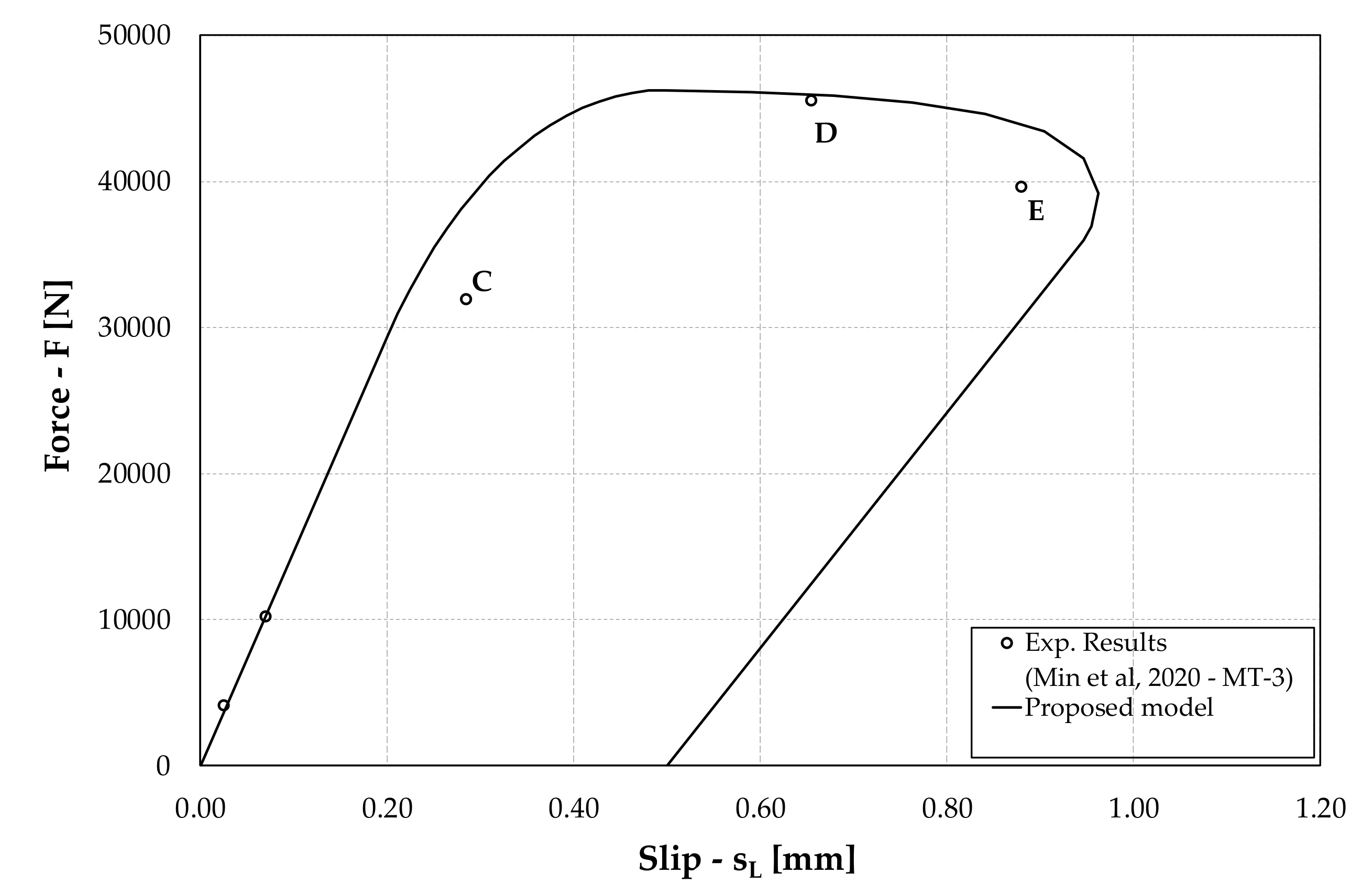
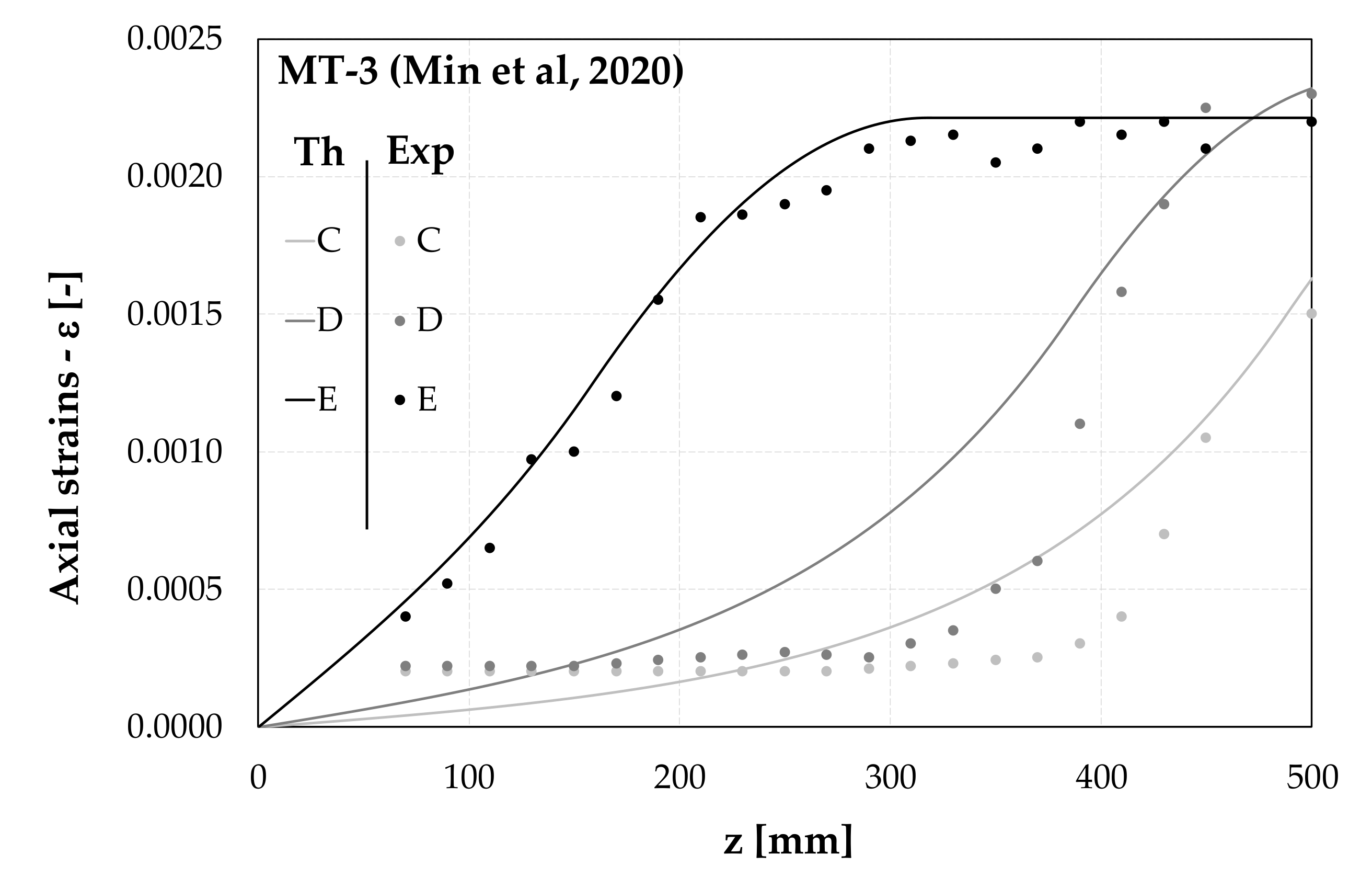
3.2. Pull-Out Tests by Min et al. (2020)

A set of experimental results taken from a very recent paper [17] is considered hereafter for the sake of validation of the proposed model, as both geometric and mechanical properties are significantly different with respect to the ones considered in Section 3.1. Specifically, a unidirectional Carbon Fiber-Reinforced Polymer (CFRP) plate, t_f = 1.4 mm tick and b_f = 100 mm wide, is glued to a concrete block with a bonded length of L = 500 mm. The presence of a 2-mm thick layer of epoxy resin layer makes the connection between FRP and concrete very soft in the elastic range.

Therefore, the following mechanical parameters are considered for the bilinear bond-slip law of Equation (1): s_e = 0.20 mm, s_u = 0.5 mm, and τ_max = 2.20 MPa, which, employed in the proposed simulation procedure, lead to the results represented in Figure 11 and Figure 12. Specifically, the force-slip curve represented in Figure 11 shows a very good agreement in the elastic branch, a reasonable accurate prediction of the maximum load and ultimate displacement. Needless to say, the snap-back behavior reproduced theoretically cannot be observed in the considered experimental tests.

Similarly, Figure 12 shows that the distribution of axial strains determined for the three different values of the imposed displacement already emphasized in the force-slip curve of Figure 11 (namely, points C, D and E) are in good agreement, especially in the final stage (Point E), with the corresponding experimental observations.

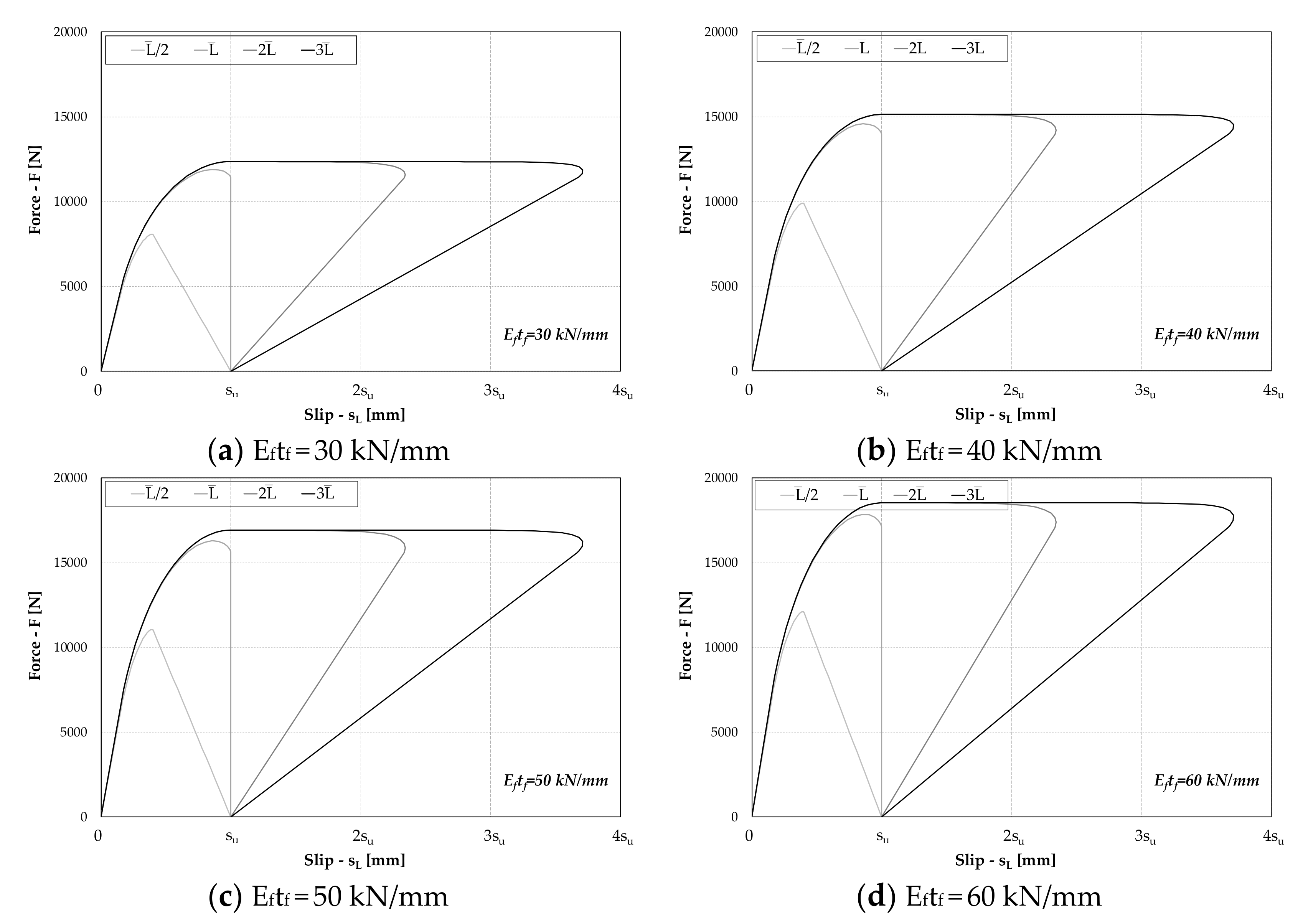
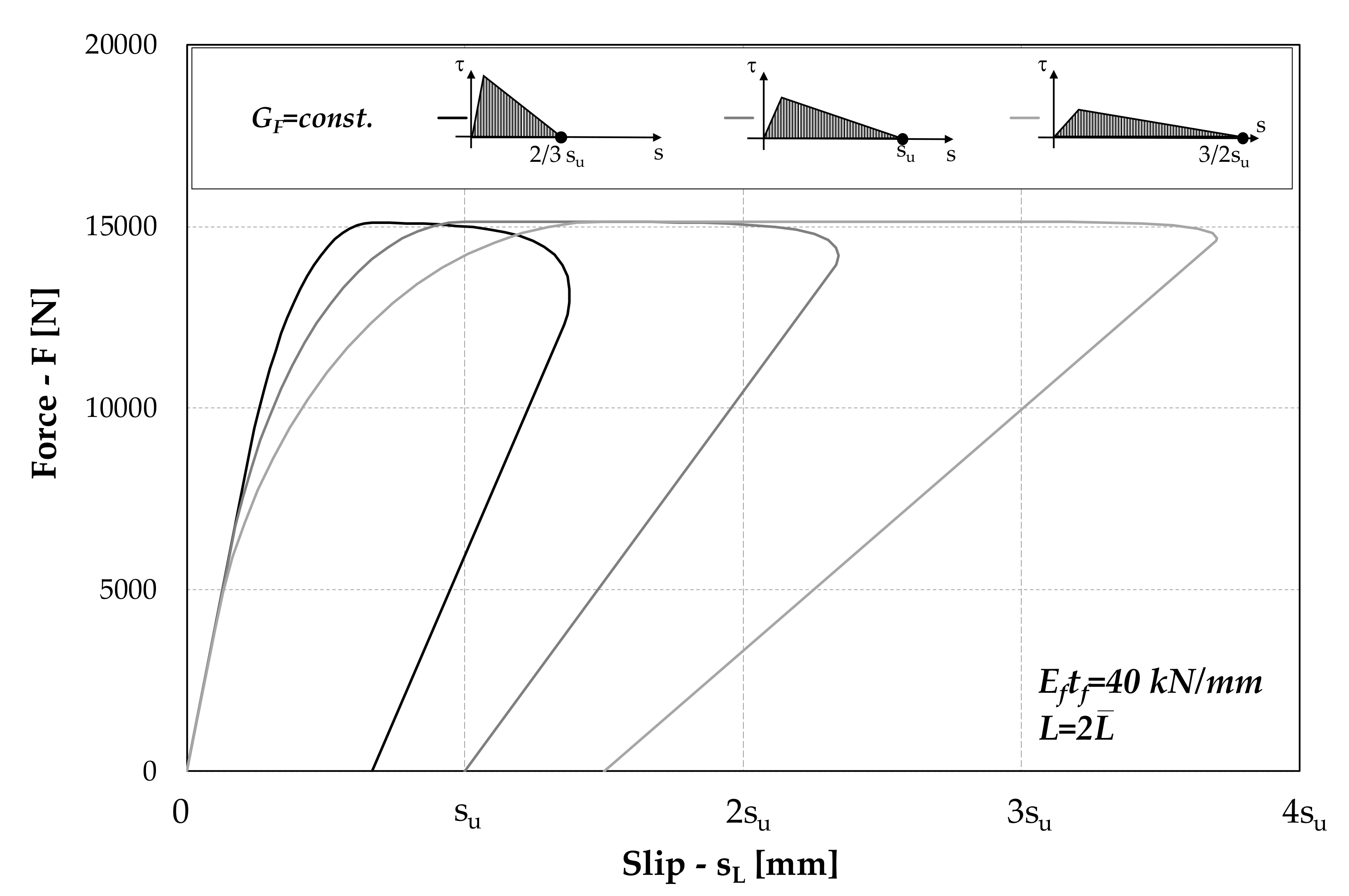
4. Parametric Analysis

Some further analyses can be carried out with the aim of showing the influence of the variation of different parameters on the resulting force-slip curve. The starting point of this study is an “average” bond-slip law among those assumed in Section 3.1 (and already considered in a previous study [16]): s_e = 0.05 mm, s_u = 0.33 mm, and τ_max = 6.93 MPa. Moreover, with the aim of considering a case of practical relevance, the following properties are firstly considered for the composite b_f = 50 mm and E_ft_f = 40 kN/mm (ideally corresponding to E_f = 240 GPa and t_f = 0.167 mm). In these conditions, α_u² = 6.18 × 10⁻⁴ according to the definition given in Equation (6), and hence the critical transfer length $\overline{L}$ = 63.21 mm can be obtained from Equation (21).

A first series of analyses will be intended to show the influence of the bond length L on the resulting force-slip curve. To this end, the following four values will be considered $L=\overline{L}/2$, $L=\overline{L}$, $L=2\overline{L}$, and $L=3\overline{L}$.

The four diagrams in Figure 13 show the results of the analyses. On the one hand, each one of the graphs, related to a given value of the specific membrane stiffness E_ft_f of the FRP plate, show the transition from short anchorage ($L=\overline{L}/2$), in which case a softening behavior is obtained, to long anchorage $L\ge \overline{L}$, characterized by a more or less pronounced snap-back response. It is worth highlighting that the proposed solution scheme does not require any complicated numerical control to handle the snap-back response in terms of F-s_L relationship: this is because the control displacement is not s_L, but s₀, the latter simply ranging from 0 to s_u throughout the whole analysis process. On the other hand, the synoptic vision of the four graphs shows that, for each value of L, the response in terms of displacements is not affected by the variation in E_ft_f; it should, however, be clear that for each value of E_ft_f a corresponding value of $\overline{L}$ is determined consistently with its definition provided in Equation (21). As is well-known from the literature [18], the force F is as high as the square root of the specific membrane stiffness E_ft_f; this relationship can be easily recognized in the graphs of Figure 13, as, for instance, the maximum force for E_ft_f = 60 kN/mm is $\sqrt{2}$ times the one determined in the case of E_ft_f = 30 kN/mm.

Further analyses can be carried out with the aim to point out the role of the “shape” of the bond-slip law, though assuming an invariant value of fracture energy G_F.

Starting from the bond-slip law identified by the values introduced at the beginning of Section 4, two variations can be determined by dividing and multiplying, respectively, the value of s_u by a 3/2 factor and modifying s_e and τ_max for the resulting value of G_F (which is the area underneath the bilinear curve), which is actually invariant.

The three bond-slip laws are depicted in the legend reported in the upper part of Figure 14 that also shows also the resulting force-slip curves. As expected, since both E_ft_f and G_F are invariant in the three analyzed cases the curves achieve the same maximum force. However, since the three bond-slip curves happen to have different values of k_u and hence α_u, each one of them is characterized by different values of $\overline{L}$. Therefore, although they all have a bond length value parametrically defined as $L=2\overline{L}$, the bond-slip characterized by lower values of ultimate slip capacity results in lower ultimate slip also in terms of global F-s_L response.

5. Conclusions

This paper presented a novel solution scheme for obtaining closed-form expressions capable of simulating the response of FRP-to-concrete joints subjected to pull-out actions. The procedure is driven by controlling the displacement at the free end, which leads to a cascading solution scheme of the differential equations describing the behavior of the various parts of the interface, taking into account their actual state of stress described by either the elastic, softening, or debonded branch of the bilinear bond-slip law assumed in this study and widely accepted in the literature.

The most significant findings of this study are highlighted below:

-

The closed-form expressions obtained by assuming a cascading piecewise solution scheme are much simpler that the one presented in a previously co-authored paper [22];

-

The assumption of the free-end slip as the main controlling displacement parameters made it much easier to handle both the softening and snap-back response deriving, in principle, from the two cases of short and long anchorage, respectively;

-

The proposed results of parametric analyses pointed out some noteworthy relationships between the relevant geometric and mechanical parameters of the bond-slip law and the resulting force-slip response of the FRP-to-concrete joint;

-

Particularly, it pointed out the key importance of the critical the value $\overline{L}$ of the of the bond length L depending on both the bond-slip parameters and the specific membrane stiffness of the composite strip.

Finally, it is worth highlighting that since the proposed closed-form solution does not require any iterative process, it is particularly efficient in terms of computational costs, and hence it is well suited to be utilized in indirect identification procedures of bond-slip laws of FRP strips glued on materials such as concrete, masonry, or steel.

References

1. Zoghi, M. The International Handbook of FRP Composites in Civil Engineering; CRC Press: Boca Raton, FL, USA, 2013. [Google Scholar]
2. Teng, J.; Cheng, J.; Smith, S.; Lam, L. FRP-Strengthened RC Structures; Wiley: Chichester, UK, 2002. [Google Scholar]
3. Seracino, R.; Griffith, M.C. FRP-Strengthened Masonry Structures, 1st ed.; CRC Press: Boca Raton, FL, USA, 2014. [Google Scholar]
4. Zhao, X.-L. FRP-Strengthened Metallic Structures; Apple Academic Press: Palm Bay, FL, USA, 2013. [Google Scholar]
5. Schober, K.-U.; Harte, A.M.; Kliger, R.; Jockwer, R.; Xu, Q.; Chen, J.-F. FRP reinforcement of timber structures. Constr. Build. Mater. 2015, 97, 106–118. [Google Scholar] [CrossRef] [Green Version]
6. CNR. DT 200/R1—Guide for the Design and Construction of Externally Bonded FRP Systems for Strengthening Existing Structures: Materials, RC and PC Structures, Masonry Structures, R1 Version, Italian National Research Council. 2005. Available online: https://www.cnr.it/en/node/2636 (accessed on 1 November 2020).
7. CNR. DT 201—Guide for the Design and Construction of Externally Bonded FRP Systems for Strengthening Existing Struc-tures: Timber Structures, Preliminary Study, Italian National Research Council. 2013. Available online: https://www.cnr.it/en/node/2637 (accessed on 1 November 2020).
8. CNR. DT 202—Guide for the Design and Construction of Externally Bonded FRP Systems for Strengthening Existing Struc-tures: Timber Structures, Preliminary Study, Italian National Research Council. 2013. Available online: https://www.cnr.it/en/node/2638 (accessed on 1 November 2020).
9. Cauich, P.J.P.; Martínez-Molina, R.; Marrufo, J.L.G.; Franco, P.J.H. Adhesion, strengthening and durability issues in the retrofitting of Reinforced Concrete (RC) beams using Carbon Fiber Reinforced Polymer (CFRP)—A Review. Rev. ALCONPAT 2019, 9, 130–151. [Google Scholar] [CrossRef] [Green Version]
10. Funari, M.F.; Lonetti, P. Initiation and evolution of debonding phenomena in layered structures. Theor. Appl. Fract. Mech. 2017, 92, 133–145. [Google Scholar] [CrossRef]
11. Funari, M.F.; Spadea, S.; Fabbrocino, F.; Luciano, R. A Moving Interface Finite Element Formulation to Predict Dynamic Edge Debonding in FRP-Strengthened Concrete Beams in Service Conditions. Fibers 2020, 8, 42. [Google Scholar] [CrossRef]
12. Kang, T.H.-K.; Howell, J.; Kim, S.; Lee, D.J. A State-of-the-Art Review on Debonding Failures of FRP Laminates Externally Adhered to Concrete. Int. J. Concr. Struct. Mater. 2012, 6, 123–134. [Google Scholar] [CrossRef] [Green Version]
13. Faella, C.; Martinelli, E.; Nigro, E. Formulation and validation of a theoretical model for intermediate debonding in FRP-strengthened RC beams. Compos. Part B Eng. 2008, 39, 645–655. [Google Scholar] [CrossRef]
14. Bennati, S.; Colonna, D.; Valvo, P.S. A cohesive-zone model for steel beams strengthened with pre-stressed laminates. Procedia Struct. Integr. 2016, 2, 2682–2689. [Google Scholar] [CrossRef]
15. Lu, X.; Teng, J.; Ye, L.; Jiang, J. Bond-slip models for FRP sheets/plates externally bonded to concrete. Eng. Struct. 2006, 27, 920–937. [Google Scholar] [CrossRef]
16. Chajes, M.; Finch, W.; Januska, T.; Thomson, T. Bond and force transfer of composite material plates bonded to concrete. ACI Struct. J. 1996, 93, 208–217. [Google Scholar]
17. Min, X.; Zhang, J.; Wang, C.; Song, S.; Yang, D. Experimental Investigation of Fatigue Debonding Growth in FRP–Concrete Interface. Materials 2020, 13, 1459. [Google Scholar] [CrossRef] [PubMed] [Green Version]
18. Faella, C.; Martinelli, E.; Nigro, E. Direct versus Indirect Method for Identifying FRP-to-Concrete Interface Relationships. J. Compos. Constr. 2009, 13, 226–233. [Google Scholar] [CrossRef]
19. Faella, C.; Martinelli, E.; Nigro, E. Interface Behaviour in FRP Plates Bonded to Concrete: Experimental Tests and Theoretical Analyses. In Advanced Materials for Construction of Bridges, Buildings, and Other Structures III; Mistry, V., Azizinamini, A., Hooks, J.M., Eds.; ECI Symposium Series: New York, NY, USA, 2003; Volume P05, Available online: https://dc.engconfintl.org/advanced_materials/3 (accessed on 1 November 2020).
20. Yuan, H.; Teng, J.; Seracino, R.; Wu, Z.; Yao, J. Full-range behaviour of FRP-to-concrete bonded joints. Eng. Struct. 2004, 26, 553–565. [Google Scholar] [CrossRef]
21. Chen, F.; Qiao, P. Debonding analysis of FRP–concrete interface between two balanced adjacent flexural cracks in plated beams. Int. J. Solids Struct. 2009, 46, 2618–2628. [Google Scholar] [CrossRef] [Green Version]
22. Caggiano, A.; Martinelli, E.; Faella, C. A fully-analytical approach for modelling the response of FRP plates bonded to a brit-tle substrate. Int. J. Solids Struct. 2012, 49, 2291–2300. [Google Scholar] [CrossRef] [Green Version]
Figure 1. Bilinear bond-slip law.
Fibers 09 00022 g001
Figure 2. Configuration of the mechanical system and representation of a segmental element of a Fiber-Reinforced Polymer (FRP) strip.
Fibers 09 00022 g002
Figure 3. Theoretical vs. experimental comparisons in terms of axial strains (2-in. specimen [16]).
Fibers 09 00022 g003
Figure 4. Theoretical vs. experimental comparisons in terms of axial strains (4-in. specimen [16]).
Fibers 09 00022 g004
Figure 5. Theoretical vs. experimental comparisons in terms of axial strains (6-in. specimen [16]).
Fibers 09 00022 g005
Figure 6. Theoretical vs. experimental comparisons in terms of axial strains (8-in. specimen [16]).
Fibers 09 00022 g006
Figure 7. Theoretical vs, experimental comparisons in terms of interface shear stresses (2-in. specimen [16]).
Fibers 09 00022 g007
Figure 8. Theoretical vs, experimental comparisons in terms of interface shear stresses (4-in. specimen [16]).
Fibers 09 00022 g008
Figure 9. Theoretical vs. experimental comparisons in terms of interface shear stresses (6-in. specimen [16]).
Fibers 09 00022 g009
Figure 10. Theoretical vs. experimental comparisons in terms of interface shear stresses (8-in. specimen [16]).
Fibers 09 00022 g010
Figure 11. Theoretical vs. experimental comparisons in terms of force-slip curve (MT-3 specimen [17]).
Fibers 09 00022 g011
Figure 12. Theoretical vs. experimental comparisons in terms of axial strain distribution (MT-3 specimen [17]).
Fibers 09 00022 g012
Figure 13. Influence of the variations of both the specific membrane stiffness Eftf and the bond length L.
Fibers 09 00022 g013
Figure 14. Influence of the variation in the shape of the bond-slip law (GF invariant).
Fibers 09 00022 g014
Publisher’s Note: MDPI stays neutral with regard to jurisdictional claims in published maps and institutional affiliations.