Article

Characterization and Simulation of Acoustic Properties of Sugarcane Bagasse-Based Composite Using Artificial Neural Network Model

by
Virginia Puyana-Romero
1,2,
Jorge Santiago Arroyo Chuquín
1,
Saúl Israel Méndez Chicaiza
1 and
Giuseppe Ciaburro
3,*
1
Department of Sound and Acoustic Engineering, Universidad de Las Américas, Quito EC170125, Ecuador
2
Laboratory of Acoustic Engineering, Universidad de Cádiz, 11510 Puerto Real, Spain
3
Department of Architecture and Industrial Design, Università degli Studi della Campania Luigi Vanvitelli, 81031 Aversa, Italy
*
Author to whom correspondence should be addressed.
Fibers 2023, 11(2), 18; https://doi.org/10.3390/fib11020018
Submission received: 14 November 2022 / Revised: 22 January 2023 / Accepted: 1 February 2023 / Published: 3 February 2023

Abstract

:
Environmental sustainability and environmental protection represent essential challenges for the well-being of the community. The use of eco-sustainable materials in architecture is necessary for the transformation of urban centers into modern sustainable cities, to reduce air pollution and protect natural ecosystems, decrease greenhouse gas emissions and improve the energy efficiency of buildings. In this study, sugar cane processing waste was used as an alternative and ecological acoustic material, combining it with natural binders used in construction, such as plaster and clay. To make the composite, the fibers were separated from the bark, then the fibers were assembled with the binder in the frames, and finally the frame with the composite was subjected to a drying process. Specimens of various thicknesses were prepared and the sound absorption coefficient (SAC) at normal incidence was calculated. Subsequently, to compare the acoustic performances of the samples, a simulation model for the prediction of the SAC based on the artificial neural network (ANN) was created. The results suggest the adoption of the simulation model to review the acoustic properties of the material.

1. Introduction

In the historical period we are living in, environmental sustainability and environmental protection are crucial issues. From this perspective, growing attention is being given to addressing the environmental emergency with sustainable solutions that can respond efficiently to the needs of new architectural technologies, while respecting nature [1]. To this end, many public administrations and organizations around the world are implementing policies oriented towards the eco-efficiency of the built environment [2].
Limitations suggested by environmental protection related to the need to ensure human health and wellbeing serve as a new catalyst for product innovation as a means of raising standards and ensuring biocompatibility and ecological sustainability. Our planet’s capacity for development depends directly on the resources still available and on its ability to absorb man-made waste. This has consequences on an economic level since the limits to growth are strictly dependent on the availability of resources and the ability to manage waste. The recent condition is exemplified by a rapid depletion of the former and an inevitable increase of the latter [3]. Sustainable development therefore requires a radical change in consumption patterns and lifestyles, requiring the reduction of the waste of materials and energy in the production of goods and the reduction of waste and emissions into the environment. From this perspective, the recovery of waste materials represents an opportunity that the construction sector cannot pass up [4].
The problem of waste management and disposal has been the subject of increasing attention. The increase in urbanization and the growth in consumption have led to a greater production of waste [5]. To deal with the problem, criteria and methods of intervention have been defined. One approach to reduce material waste is reuse and recycling [6]. The topic of recycling is not new, but represents a common practice in human history. Archaeological studies of ancient landfills reveal the presence of a small amount of household waste in times when resources were scarce, testifying to the recycling of materials [7]. Nowadays, more and more attention is required for the reuse and recycling of materials, taking advantage of the life cycle assessment (LCA); on the one hand, LCA represents one of the fundamental tools for the implementation of a product policy, while on the other hand, it is an objective way of assessing the energy and environmental loads and potential impacts associated with a product throughout its life cycle [8]. The relevance of the recycling technique essentially lies in its innovative approach, which consists in evaluating all phases of a production process as correlated and dependent. New buildings are now being constructed based on LCA, and recyclable or eco-sustainable materials interact to meet system needs [9].
Fibers are characterized by flexibility, fineness and high ratio between length and maximum transverse dimension (diameter), which make it suitable for use in the production of building materials [10]. Natural fibers are already fibrous in their unprocessed state; handling does not alter their chemical makeup. In comparison to synthetic fibers, natural fibers are less expensive, easier to handle, have high mechanical qualities, use less energy during production, and are biodegradable [11]. Due to current issues with waste disposal and the depletion of petrochemical resources, increased environmental awareness has played a significant role in the creation of composite materials using natural fibers. The use of natural materials in modern buildings can reduce waste, increase energy efficiency and at the same time promote the concept of sustainability. Natural fibers are obtained from different parts of the plant. They can be extracted from the stem, leaf, seeds, or fruit of the plants themselves [12].
Vegetable waste includes biodegradable waste such as kitchen and garden waste, but also waste related to tree pruning or grass cutting, ending with crop waste. Vegetable waste is usually treated in composting or fermentation plants in order to be transformed into compost, digestate and biogas, respectively. A different solution for such waste could be their reuse to produce new materials [13]. One such vegetable fiber waste is sugar cane bagasse (SCB), an organic waste from sugar cane, for which various applications have been developed [14]. Bagasse can be used as a building material, mixing it with traditional materials, thus allowing an improvement in properties. Han et al. [15] used waste from sugar cane cultivation to produce structural composites using wood strands. The two fibers were bonded with phenol formaldehyde resin, obtaining a composite with structural properties improved with respect to the starting compounds. Bilba et al. [16] used SCB fibers, enhanced with a silane coating, as a reinforcing material in a cement matrix. The authors showed that the setting time increases with the silane coating in reinforced composites with non-pyrolyzed bagasse fibers. The combination of pyrolysis and silane treatment improves the water resistance of the fibers, which become more hydrophobic. Doherty et al. [17] studied the use of the lignin contained in the SCB as a coating of a composite. The authors showed that the resin films of the lignin represent an effective barrier to water. Trindade et al. [18] used SCB to produce phenolic thermosetting composites. The authors created quinones in the lignin portions of the fiber and reacted them with furfuryl alcohol to create a coating around the SCB that is more compatible with the phenolic resins used to prepare the polymer matrix. Frias et al. [19] investigated the influence of the calcination temperature on the pozzolanic activation of SCB. The authors showed that the SCB calcined at 800 °C and 1000 °C has properties indicative of very high pozzolanic activity, while they found no influence of the calcination temperature on pozzolanic activity. Mulinari et al. [20] developed a composite using SCB with a matrix of a high-density polyethylene polymer. The composite obtained shows a lower tensile strength than the starting polymer, while an increase in Young’s modulus was found due to the reinforcement of the fibers, with an increase in structural defects that can be reduced with the use of modified cellulose fibers.
Noise represents one of the most important causes of the deterioration of the quality of life and is now recognized as a major environmental problem [21]. Acoustic absorption has the purpose of partially neutralizing sound waves, the reflection of which varies according to the type of structure and its reaction to sound energy, in order not to disturb nearby environments and not be disturbed [22]. Acoustic insulation can be defined as the action or set of actions in favor of the attenuation of noise from one environment to another, be it airborne noise, footfall noise or vibration [23]. The choice of acoustically insulating and absorbing materials therefore becomes crucial to ensure acoustic comfort in buildings. Doost-Hoseini et al. [24] studied the correlation between the physical and mechanical properties and the acoustic characteristics of insulating panels made of SCB. The raw material was bound with different types of resins: urea-formaldehyde (UF) and melamine-urea-formaldehyde (MUF). The authors demonstrated that resin type had no significant effect on physical or mechanical properties, while it did affect SAC. The density of the material produced characterized the physical and mechanical properties, while the SAC was influenced by the type of panel. The study showed a high correlation between physical and mechanical properties and a low correlation between physical and mechanical properties with SAC values. Mehrzad et al. [25] fabricated fibrous samples of different densities and thicknesses using SCB. They next investigated the sound absorption capacity of the samples with the impedance tube technique. The authors achieved good sound absorption performance in the low- and mid-frequency ranges. Malawade et al. [26] measured the SAC of SCB samples. The test samples were made from raw dried bagasse without chemical treatment and physical modifications. The authors measured SAC and the resistivity of the airflow. The results show that the SAC and flow resistivity increase with increasing SCB sample thickness. Othmani et al. [27] investigated the acoustic performance of the SCB by measuring two acoustic parameters: flow resistivity and SAC. The authors produced several specimens by binding the bagasse fibers with resins; different combinations, varying fiber size, specimen thickness, and resin content, were predicted. The results allowed the effect of each property on the acoustic performance of the studied material to be evaluated. The results showed good agreement between experimental and theoretical results.
For the study of the acoustic properties of materials, it is essential to carry out measurements of the SAC according to what is indicated by the technical standards. Alongside the experimental measurement procedure, it is advisable to carry out a simulation study that allows for an investigation of what is and what is not possible or economically viable [28,29]. In recent times, more and more scholars are approaching simulation studies with a data-driven approach. In this case, the simulation process is guided by the data collected in the measurement campaigns and allows us to guide the decision-making process. In this context, machine-learning-based algorithms offer us the tools to extract knowledge from automatically collected data [30,31]. Artificial neural networks (ANN) are a subgroup of machine learning and are inspired by the human brain. The basic idea is to mimic the way biological neurons send each other signals [32]. ANNs reflect human behavior, letting computer programs to identify patterns and resolve ordinary problems in fields of artificial intelligence [33]. ANNs depend on training data to learn and improve their accuracy over time. If improved in accuracy, these algorithms are effective tools, permitting us to classify and cluster data at high speed [34].
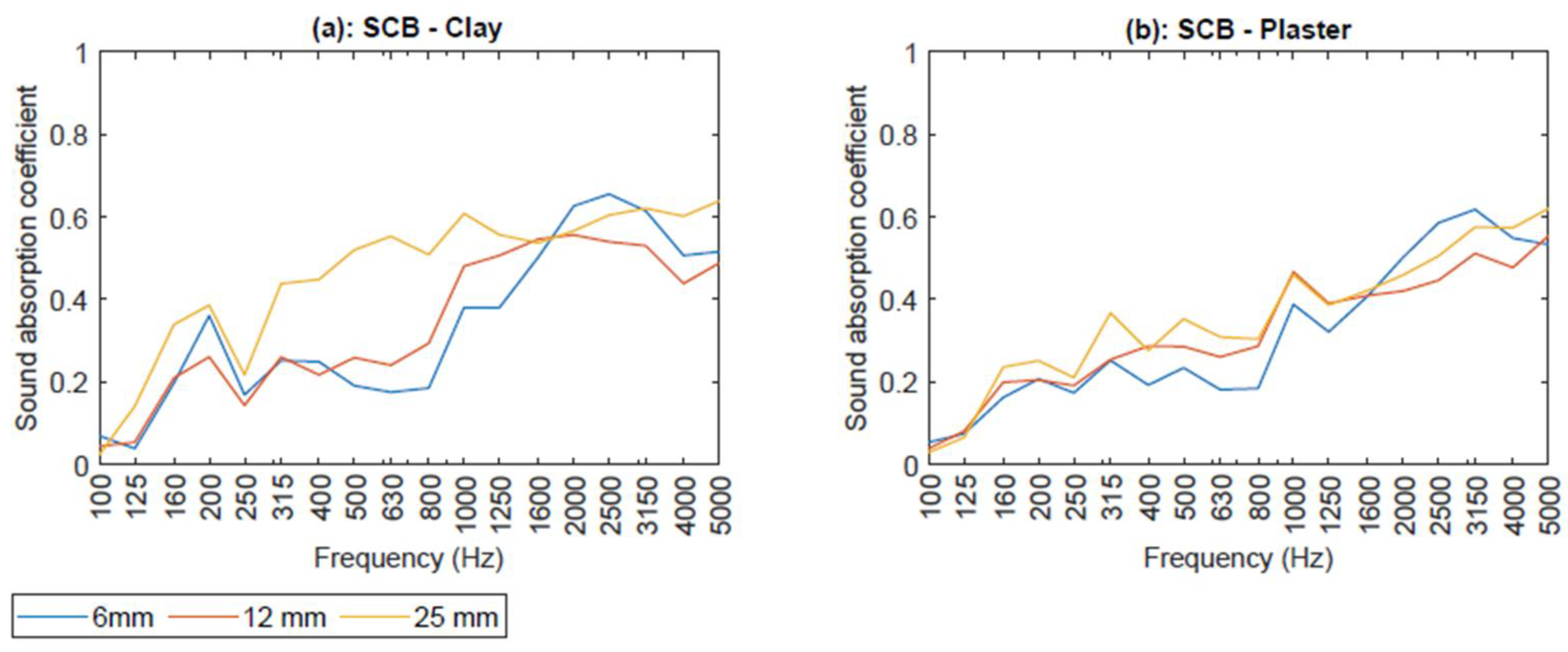
In this study, the potential of SCB as an alternative and ecological acoustic material was analyzed, combining it with binders used in construction such as plaster and clay. To make the panels, the SCB was mixed with the binder in different ratios, according to the binder used. In this way, a panel was obtained in which the bagasse was predominant. Samples of three thicknesses 6, 12 and 25 mm were made with each binder. The sound absorption coefficient of the samples was then measured according to the guidelines of the UNE-EN ISO 10534-2 standard [35]. Subsequently, to compare the acoustic performances of the samples, a simulation model was developed for the prediction of the SAC.
The paper is structured as follows. Section 2 illustrates the materials and methodologies applied. First, the methodologies utilized to create the samples from the waste material of sugar cane cultivation are explained. Consequently, the procedures for measuring the sound absorption coefficient with the impedance tube technique are described. Therefore, the methodologies used to elaborate the simulation model based on the ANN are described. Section 3 shows the results achieved from the measurements of the SAC and subsequently compares them with the results obtained with the simulation model based on ANNs. Finally, Section 4 recapitulates the results achieved from this work and examines the possible uses of the developed technology in real cases.

2. Materials and Methods

Sugar cane (Saccharum officinarum), a plant of the Poaceae family, is considered one of the main products of Latin America [36]. The country that produces the largest amount of sugar cane is Brazil (46.7%) followed by India (19.8%) and then China (8.1%) [37]. In the production areas (tropical/equatorial) characterized by periodic rains, the planting period must be determined based on the rain cycle; usually the sowing takes place at the beginning of the rainy season, with the first harvest, which takes place after about nine months, taking advantage of the two or three months of the dry season. The next crop is obtained from the remains of the basal part of the cut canes, and the canes reach commercial maturity after a few months (5–6) for the next cut.
Sugar cane is made up of juice and fiber. The juice is made up of soluble solids called brix, while the fiber is the insoluble part of sugar cane which is made up of cellulose. In addition to components such as brix in its percentage form, there are organic and inorganic components such as salts, minerals, proteins, and others. The sap of the stem, which acts as a reserve element for the plant, contains a high percentage of sucrose (up to 18–20%), which accumulates before being translocated either to the root system or towards the flower and the fruit in case the plant flowers. Sugar is industrially extracted by crushing the cane and crystallizing the soluble solids [38]. The extraction takes place directly by pressing the mature segments of cane, which can be squeezed directly with a roller system or crushed and pressed with a system such as that of the presses used to obtain vegetable oils.
The origin of the word bagasse, derived from the French bagasse, was used to name the residue of the olive after being worked to extract the oil. Currently, the word bagasse is used to identify the stem of sugarcane without juice. Bagasse is made up as follows: 50% cellulose, 5% soluble solids and 45% crude fiber. Bagasse is therefore the waste product in the process of extracting sugar from sugar cane. In general, 280 kg of wet bagasse (28%) are produced from 1 tonne of sugar cane [39]. As a result, converting SCB into value-added products offers economic benefits and contributes considerably to environmental sustainability.

2.1. Preparation of the Samples

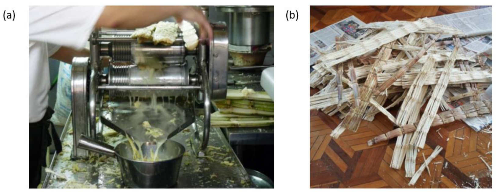
The collection of the raw material was carried out in the province of Imbabura in Ecuador, where sugar cane waste abounds. In this province, sugar cane juice is extracted using juicer machines (Figure 1a) and eventually its scraps are thrown into the garbage. Sugar cane waste (Figure 1b) was collected in the municipal market of the city of Ibarra.
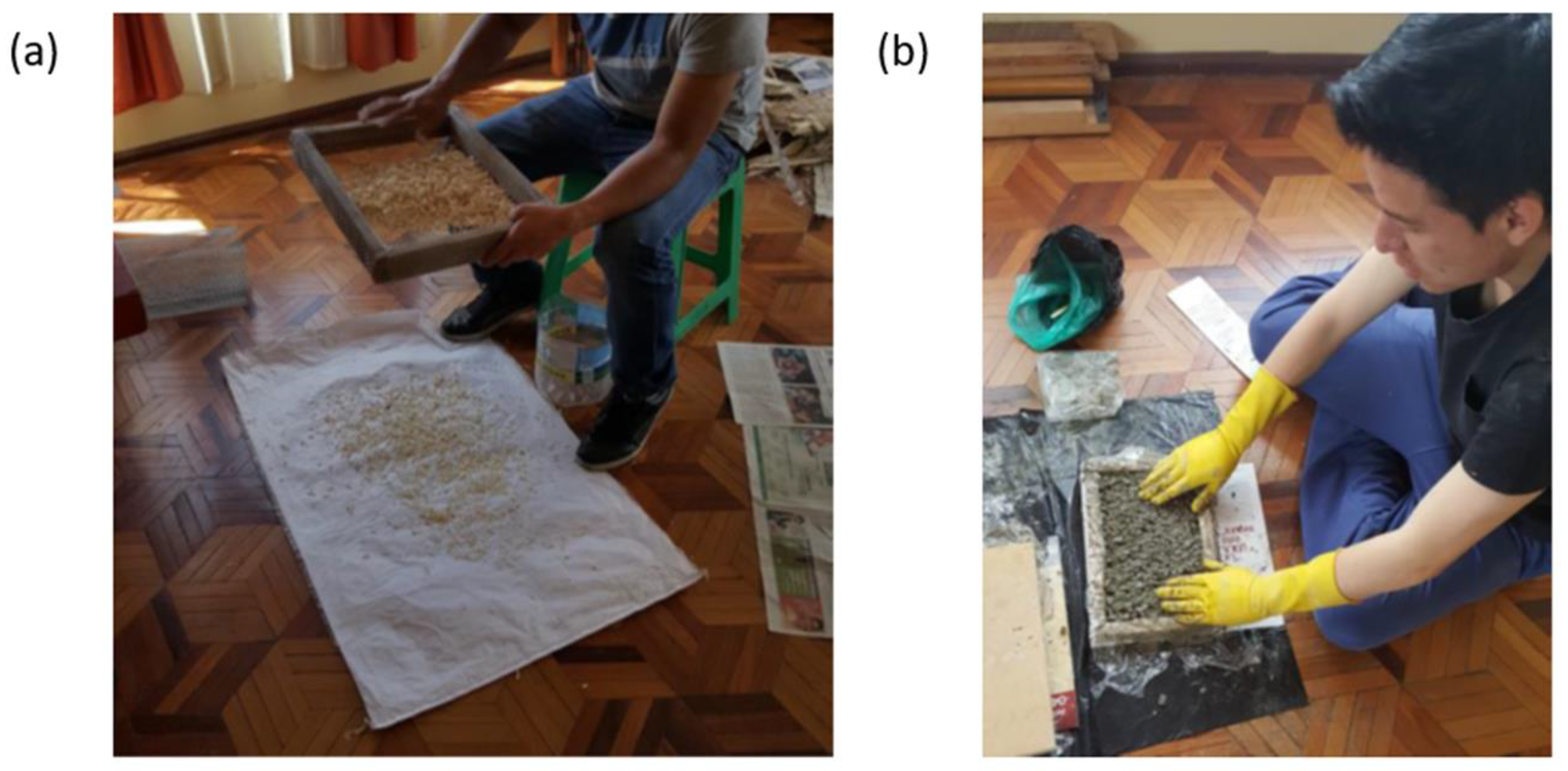
The waste product in the extraction of sugar cane juice was subjected to a preliminary drying treatment. It was decided to let the bagasse dry outdoors for a period of two days, so that its fibers did not have juice on the surface. Once the fibers dried completely, the bagasse fibers were separated from the bark. Subsequently, each of the fibers was cut to a length of approximately three to five millimeters, resulting in small pieces of bagasse fiber, which were used to make the samples.
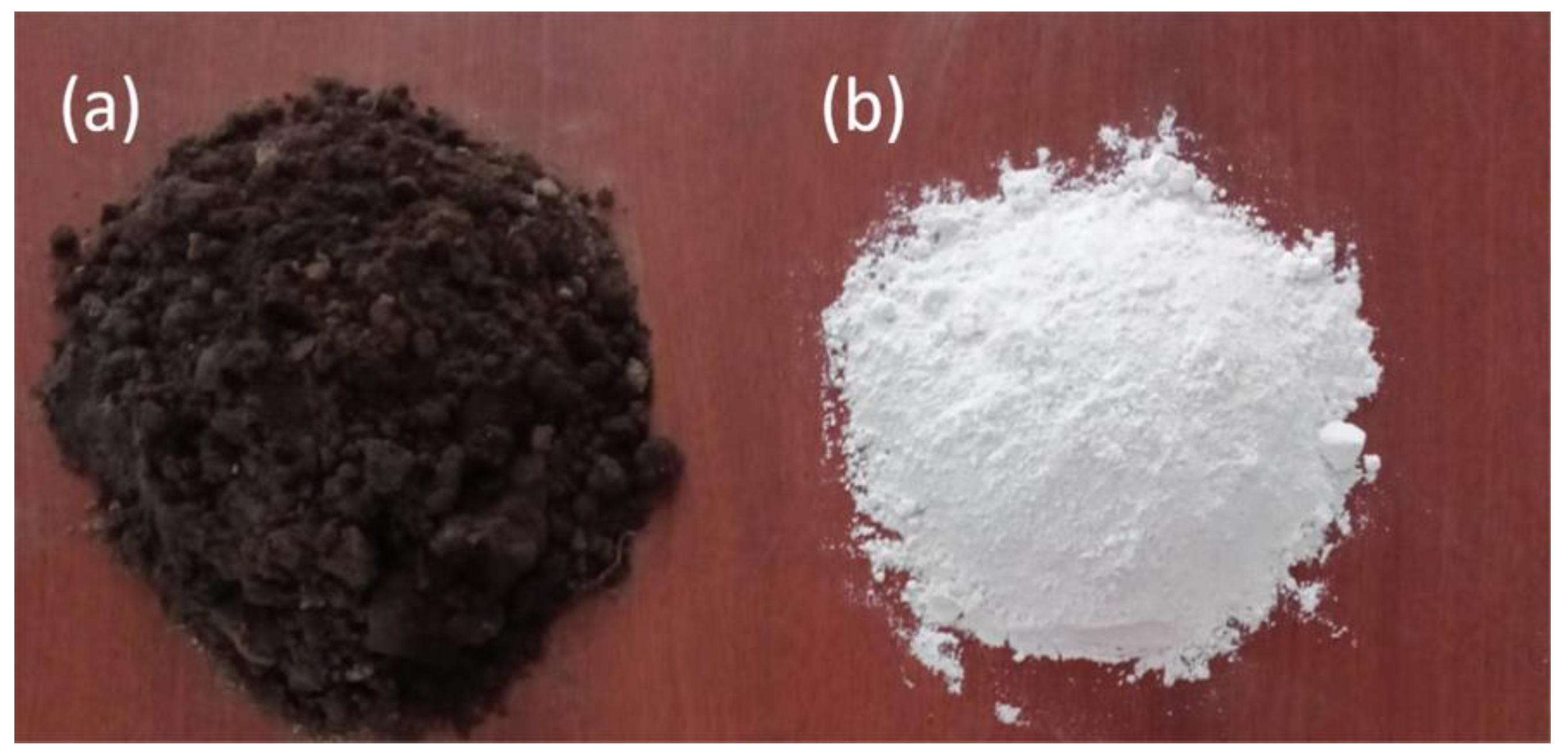
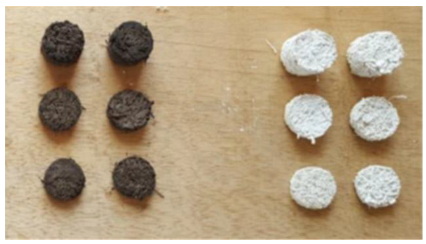
To acoustically characterize the composite material, panels with thicknesses of 6, 12 and 25 mm were assembled, in which the mixture between the bagasse and the different binders was adjusted. Figure 2 shows the two typologies of binders used.
To obtain a predominant amount of bagasse in the sample, the experiments were conducted with a bagasse to binder ratio of 3 to 1.
To ensure the reproducibility of the experiment, the following steps were followed:
  • To begin, the bagasse obtained by separating the fibers from the bark was sieved with a metal sieve, obtaining the smallest possible filaments.
  • The sieved bagasse filaments were then placed in a 15 × 25 cm size frame, making sure they completely covered the thickness of the frame, and then the amount of bagasse used in this process was weighed (Figure 3a).
  • To produce panels with SCB matrix and plaster or clay-based binders, the frame was divided into 3 parts and 1/3 of the frame is filled with the binder and then weighed. In this way, the proportions of 3/1 which had been indicated were respected. Table 1 shows the quantities of each component in the different types of assembled panels.
  • With the weights of the elements indicated in Table 1, the base elements were mixed, and placed in the respective molds (Figure 3b). The panels underwent a drying process lasting about 48 h. At the end of the drying process, the panels had assumed rigid and compact characteristics.
  • Once it had been demonstrated that the proportions of the elements were optimal for the construction of panels, the weights of the components necessary to create cylindrical-shaped samples of thicknesses equal to 6, 12 and 25 mm were calculated, to be used for the measurement of the coefficients of sound absorption using the impedance tube (Kundt tube). To obtain these samples, molds were made of the diameter allowed by the Kundt tube, which is about 35 mm. The samples were weighed on a digital scale and the weights obtained are shown in Table 2.
  • Finally, 18 samples were obtained, divided into the two binders combined with the SCB: 9 samples of SCB - plaster, and 9 samples of SCB - clay. Several similar samples were then made for each of the three foreseen thicknesses of 6, 12 and 25 mm, as shown in Figure 4.

2.2. Sound Absorption Coefficient Measurement

The samples assembled according to the procedure described in the previous section were used to measure the SAC, as required by the standard UNI EN ISO 10534-2 [35]. The method describes how to make an SAC measurement using an impedance tube (Kundt tube). It is crucial to carry out the measurements in a normalized way in order to be able to compare the results with those obtained in other studies, thus being able to compare the performance of different materials [
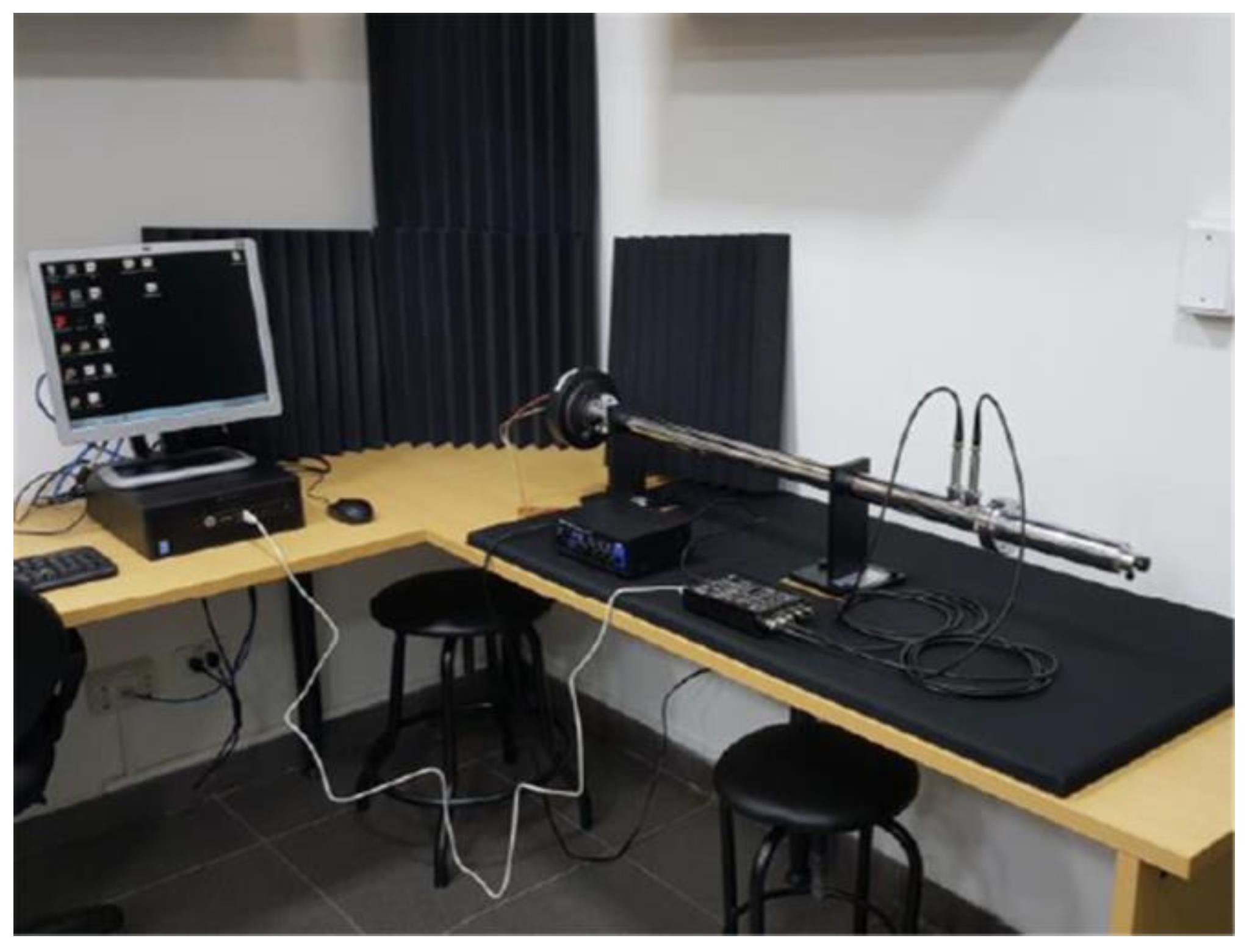
40]. In this study, the ACUPRO Spectronics impedance tube was used, which measures the sound absorption coefficient in the frequency range 50 Hz–5700 Hz. The tube has an internal diameter of 34.9 mm, while the external diameter is 41.3 mm and has a length of 1200 mm (Figure 5).
The tube features a built-in JBL 2426J speaker that emits a maximum sound pressure level of 150 dB. The mechanical insulation of the speaker guarantees the absence of structural vibrations. The tube is connected to a DT9837A signal acquisition system which manages the inputs and outputs, transforming the electrical signal into digital. The acquisition system has four input channels for data conversion and recording and an output channel for sending the signal from the computer to the speaker. The signal reproduced by the loudspeaker is captured by the two microphones and sent to the ACUPRO software for data processing. The software carries out 150 measurements by making an average and then passing to the evaluation of the sound absorption coefficient. The absorption coefficients were calculated from 100 Hz up to 5000 Hz in 1/3 octave bands.
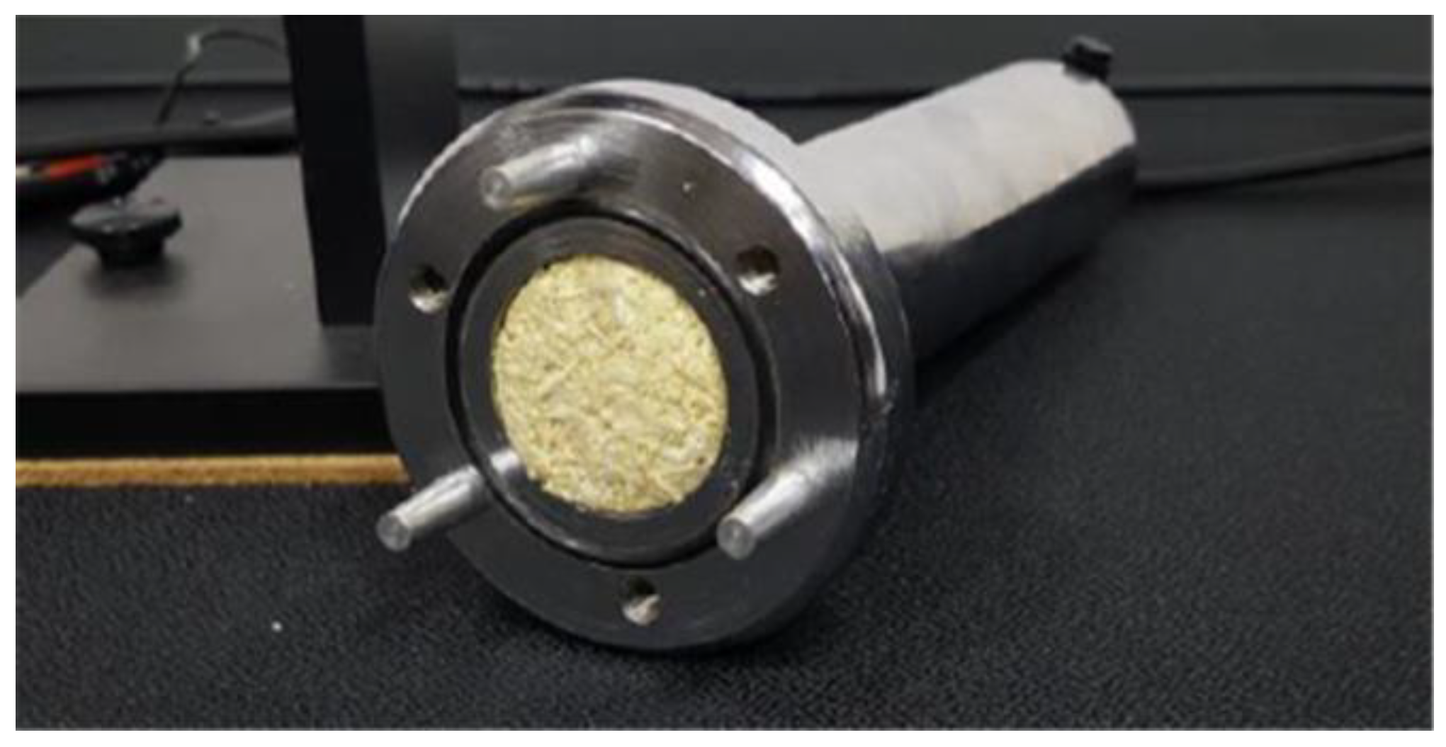
The test sample was mounted at one end of the impedance tube, using a sound source, plane waves are generated inside, and acoustic pressures are measured in two locations near the sample [41]. To normalize any irregularities in the material, 5 measurements of the same sample were carried out, replacing the sample for each measurement (Figure 6).
The complex acoustic transfer function of the signals to the two microphones is then determined, and is subsequently used to calculate the complex reflection coefficient for normal incidence, the absorption coefficient for normal incidence and the normalized impedance of the tested material [42]. The quantities determined are a function of the frequency, with a frequency resolution conditioned by the sampling frequency and the signal length of the digital frequency analysis system used for the measurements [43]. The useful frequency range depends on the width of the tube and the distance between the two microphone positions.

2.3. Artificial Neural Network (ANN) Based Modelling

Machine learning (ML) is a subfield of artificial intelligence that deals with creating systems that learn based on the data [44]. These systems train the model to correct errors so that it learns to perform a task or activity autonomously. ML works based on two distinct approaches: the computer is given complete examples to use as an indication to perform the required task (supervised learning), or the software is run without any help (unsupervised learning) [45]. In our case, having available the data obtained through the correctly labeled measures of the SAC, we will use supervised learning [46].
In this case, it is possible to distinguish between classification and regression problems. Classifiers separate data into two or more classes: When an example is given to the classifier, the algorithm returns the class to which that specific input might belong. Regressors rely on data interpolation to associate two or more characteristics with each other [47]. When the algorithm is given an input characteristic, the regressor returns the other characteristic to me. The substantial difference depends on the characteristics of the output: in the case of categorical output, we are talking about classification, but in the case of continuous output, we have a regression problem [48]. Our goal is to model the acoustic properties of SCB-based materials, since it is the SAC that has continuous values in the 0–1 range, and will then have to face a regression problem.
ANNs are based on human behavior, allowing computer programs to recognize patterns and solve common problems in ML [49,50]. The structure of the ANNs is inspired by the human brain: the idea is to mimic the way in which biological neurons send signals to each other. ANNs rely on training data to learn and improve their accuracy over time. Once optimized for accuracy, these learning algorithms are powerful tools allowing us to classify and organize data at high speed [51].
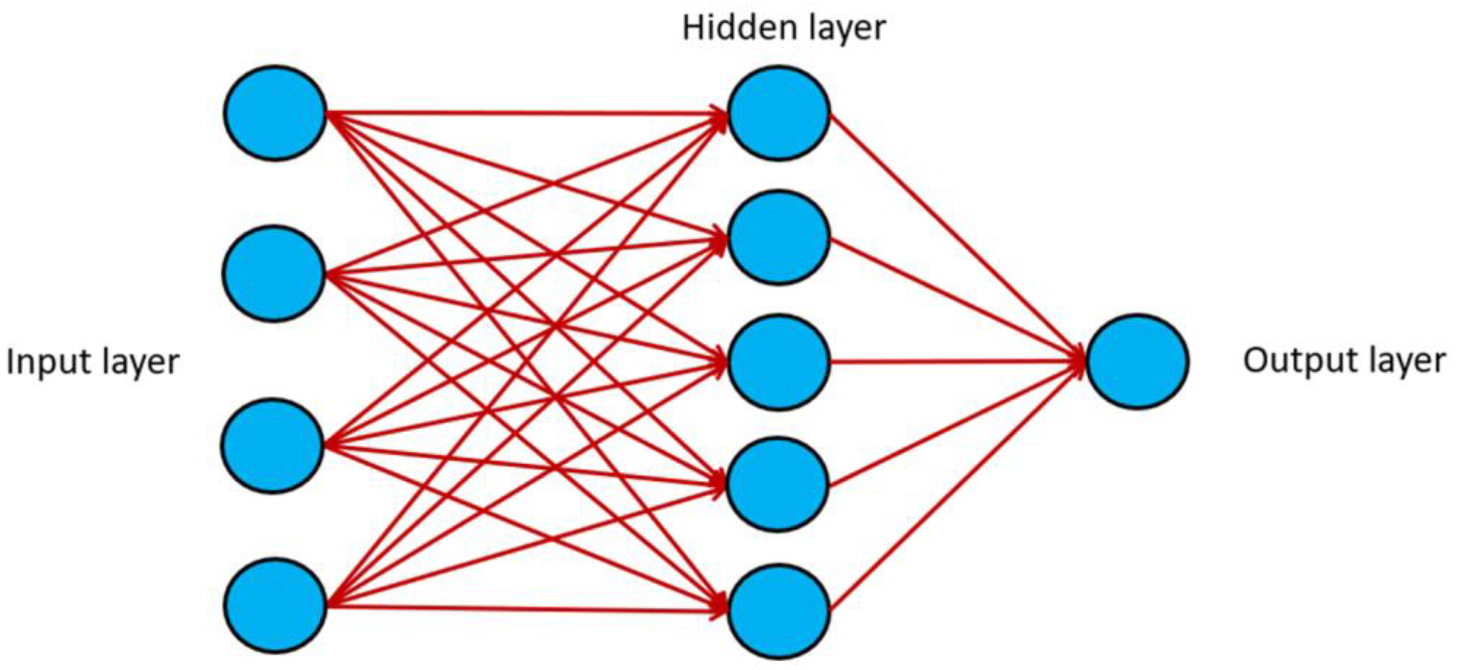
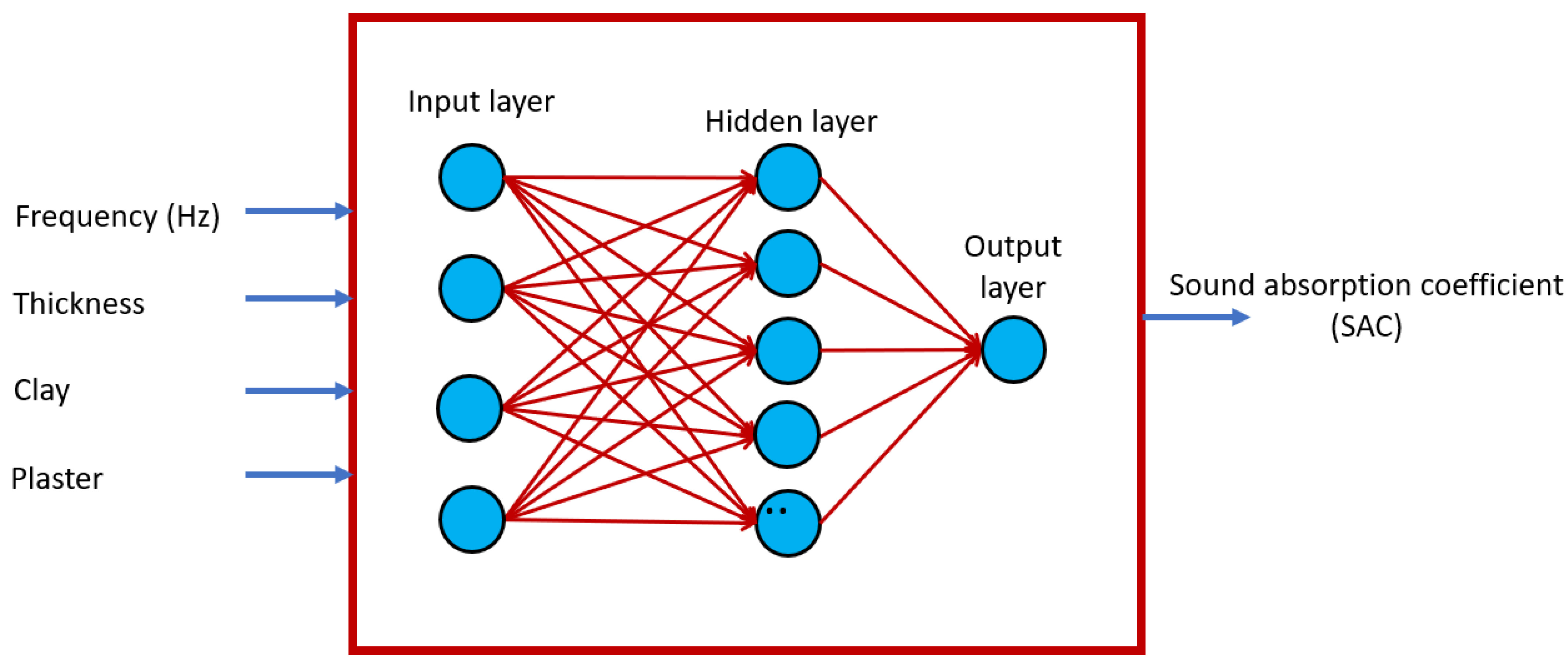
ANNs are formed of node layers that possess an input level, one or more concealed input and output layers (Figure 7). Each node bonds to another and has a corresponding weight and boundary. If the effect of any individual node is beyond the recognized threshold, that node is activated and passes on the information to the subsequent layer of the network. Otherwise, no info is transmitted to the succeeding tier of the network. From a mathematical perspective, at the base of ANNs we can translate a function as an aggregate of other functions, which in turn can be expressed in uncomplicated functions. As such, we can view an ANN as an interconnected set of fundamental functions in which the outputs are the inputs for successive functions [52].
The basic element of the ANNs is the perceptron, which performs the task that the neuron performs in biological neural networks. These elements behave like functions that take n elements in input and return only a single output, which is sent as input for the following perceptron. For this reason, we speak of stratified ANNs [53]. The input of the perceptron is formed by a vector of real numbers in which from time to time we will enter input values (x1, x2, …, xn). Furthermore, for each input node, we will have an array of weights indicated with (w1, w2, …, wn). To get the actual data we will perform a simple xn * wn operation for each input xn. The output will then be calculated using the following equation:
y = i = 1 n x i w n + b ,
Here,
  • xi = input
  • wn = weight
  • b = bias
  • y = output
Term b is called the perceptron bias and is considered a full-fledged weight. Its task is to change by increasing or decreasing the activation threshold that derives from the activation functions, for example, a function that sends a signal only if the output level of the perceptron exceeds a certain threshold [54]. In the training phase, the model adjusts the weights based on the comparison between the real values of the output and those expected. This is an optimization process in which an attempt is made to minimize a cost function represented by the output estimation error, as shown in Equation (2).
Cost   Function   = 1 2   y y 2 ,
Here,
  • y = output expected
  • y* = output predicted
The weight update rule is shown in the Equation (3):
w i = w i + μ   ϑ C o s t   f u n c t i o n ϑ w i ,
Here,
  • μ = learning rate
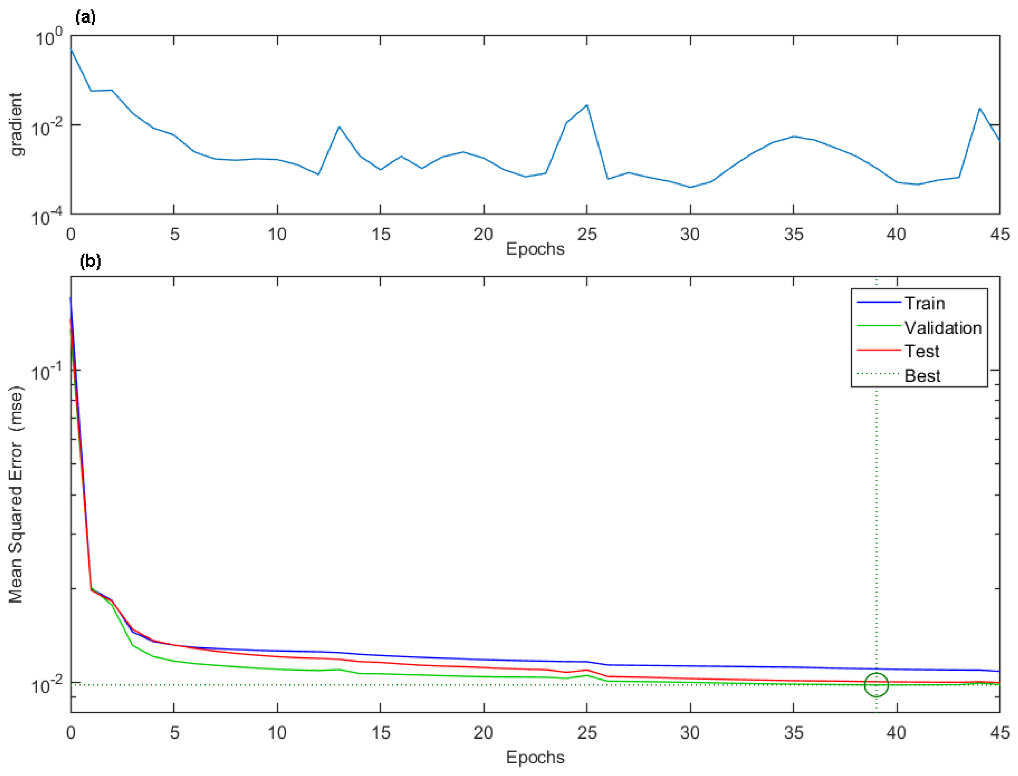
The backpropagation algorithm [55] is based totally on the gradient descent technique to locate the minimal of the error function with admire to the weights [56]. The gradient descent approach is due to the fact the gradient indicates the direction of most boom. In the basic implementation, we start by choosing a random point in multidimensional space and evaluating the gradient at that point. We then proceed by choosing another point in the direction of maximum decrease indicated by the opposite of the gradient. If the function at the second point has a value lower than the value calculated at the first point, the descent can continue, following the anti-gradient calculated at the second point, otherwise the shifting step is reduced, and starts again. The algorithm stops as soon as a local minimum is reached.

3. Results and Discussion

3.1. Sound Absorption Coefficient Measurements

The samples assembled according to the methodology described in Section 2.1 were used to perform measurements of the SAC using an impedance tube. The samples were housed in the impedance tube (Figure 6).
To acoustically characterize the behavior of the material, different measurements were carried out for each sample. For each measurement, the samples were first removed from the tube and then re-housed in it, to minimize any measurement errors. The results of the measurements were selected by discarding the extreme values, and by making an average of the values obtained. In Table 3, the standard deviation values of the measurements are reported.
Figure 8 shows the results of the measurements of the SAC for all types of samples made and for the three foreseen thicknesses. Figure 8a shows the trend of the SAC as a function of frequency in bands of one third of octaves on a logarithmic scale, for the sample based on SCB and clay-based binder. The acoustic properties of the material investigated are typical of porous materials and this characteristic is due to the peculiarities of the SCB. In fact, the SCB fibers have a high roughness which significantly contributes to sound absorption: microscopic air pockets form on the surface of the SCB fibers due to the grooved and rough surfaces. This characteristic determines a significant friction between the fibers and the incident acoustic wave, resulting in an increase in sound absorption. The roughness of the fibers also gives an increase in the surface, which increases the damping capacity of the incident wave with a relative increase in the sound absorption coefficient [57]. In this case, there are some anomalies at low frequencies due to the limits imposed by the size of the tube and to possible problems of irregularity in the production of the artisanal samples. From the comparison between the samples of smaller thicknesses (6 and 12 mm), we can see that the greater thickness determines a greater absorption starting from 1 kHz, even if the curve is the same as that of 6 mm. At low frequencies, the difficulty of the acoustic wave to penetrate the sample is due to its wavelength. For higher frequencies, both samples show upward absorption. The 25 mm sample has a much higher absorption curve than the 6 and 12 mm samples, with a relatively large difference of 10% at low frequencies and 20% at mid frequencies. Samples in general are characterized by being good absorbents, so this result can be argued by the fact that clay is a binder with good acoustic properties for insulation and absorption. The SCB fibers are intertwined and therefore create frictional forces to the movement of the sound wave within the porous material. When the sound wave penetrates the sample, friction reduces its intensity by converting the sound energy into thermal. At low frequencies, the improvement in the absorption capacity with the increase in the thickness of the sample appears evident. This increase is significant when passing from a thickness of 6 mm to that of 12 mm, while it appears less significant when passing from a thickness of 12 mm to that of 24 mm. Therefore, the sound absorption coefficient increases with the increase in the thickness of the sample and this increase is evident at low and medium frequencies. Greater wavelengths correspond at lower frequencies, which are absorbed more effectively if the sample has greater thickness: The wave path in the sample is greater and therefore the loss of sound energy due to the expansions and contractions of the molecules is greater than with air [58].
Figure 8b shows the trend of the SAC as a function of frequency in bands of one third of octaves on a logarithmic scale, for the sample based on SCB and plaster-based binder. Again, increasing the thickness of the sample leads to an increase in the sound absorption coefficient, but this increase is smaller than in the previous case. This is especially true at low frequencies, where SAC values for 6 mm and 12 mm thicknesses appear comparable for different frequencies. Such material behavior can be justified by an error generated by a poor coherence curve captured by the Acupro software, caused by the low thickness of the sample inside the tube, which leads to an incorrect result in the final measurement. This type of response will also be visible in the other samples of similar thickness with a different type of binder. From the comparison of the three samples, the effect of high degree of density that the samples of SCB bonded with plaster have, unlike the samples with SCB and glue, is highlighted. Furthermore, the adhesion that the gypsum presents allows the porosities created by the SCB to be filled. Due to this phenomenon, most of the pores are filled, generating a different absorption in the entire sound spectrum. Always at the frequency of 400 Hz, the 6 mm and 12 mm samples instead show a local peak due to resonance phenomena. The frequency of the emitting wave coincides with the natural frequency of the sample oscillation, and the sound energy picked up by the microphone inside the tube is higher than that emitted by the loudspeaker. This is due to the vibrations of the samples, which themselves become a source of sound wave emissions [59].

3.2. ANN-Based Model for SAC Prediction

The results of the measurements of the SAC contain crucial information for the modeling of the acoustic behavior of materials. This information can be extracted with technologies based on machine learning.
Various models are available in the literature for simulating the acoustic behavior of porous materials [60,61,62,63]. However, none of these can guarantee an effective generalization. In contrast, ANN-based regression models are used to study the relationship between multiple independent variables and a dependent variable (SAC). One of the major advantages of the model is the easy interpretation of the results. Furthermore, the model could determine the relative influence of one or more independent variables on the dependent variable. Limits to the effectiveness of forecasting are placed in the case of interrelated inputs, while it is appropriate to highlight the need for data preprocessing to remove missing values or redundant data.
To simulate the behavior of the SCB-based material, a model based on artificial neural networks was developed. The data obtained from the measurements of the SAC by means of an impedance tube were enriched by adding the information on the different binders used to aggregate the raw fibers. Figure 9 shows the architecture of the prediction model of the acoustic behavior of the material subject of this study.
The architecture of the ANN-based prediction model of the SAC, shown in Figure 9, provides 4 input features. To begin, we provide the frequencies for one-third octave bands in a range from 100 Hz to 5000 Hz. To these, add the thickness of the three types of assembled samples (6 mm, 12 mm, 25 mm), and then finish with the type of binder used to assemble the fibers. To include these characteristics in the regression model, we used dummy variables [64]. A dummy variable is a variable created with the purpose of using numerical values to represent qualitative variables. With a dummy variable, the data are encoded with numeric values that can only assume the value 0 or 1 (dichotomous variable). It is therefore a nominal qualitative variable which will take the value 0 to indicate that the record does not refer to that type of binder, while it will take the value 1 to indicate that the record refers to that type of binder. Therefore, for each record, only one value of the two features that indicate the type of binder will assume a value of 1, while the others will assume a value of 0. The output of the forecast model is the value of the SAC relating to the type of binder, at the thickness of the sample, and at that specific frequency. From an overall analysis of the diagram of Figure 9, it is possible to verify that the output value is a numerical and continuous type, which is why we can affirm that it is a regression problem with six predictors and a response variable. Table 4 shows the parameters of the ANN architecture.
The results of the SAC measurements were entered in a numerical dataset with five features: Four input variables (frequency, thickness, plaster, clay) and one output variable (SAC). The number of records collected with the measurements was equal to 1620, corresponding to the 18 frequencies of one third of an octave in the range 100–5000 Hz, to the three thicknesses of the samples (6 mm, 12 mm, 25 mm), and to the two types of binder (plaster, clay).
The data were carefully labeled, associating the SAC value, returned by the measurements with the impedance tube, to the correct sequence of frequencies, sample thickness and type of binder. Labeling is crucial in an ANN-based methodology of the supervised type. The label allows you to train the model using a data subset, specifying the observed output, so that at the end of the learning phase the model will have acquired the ability to generate the right label by providing it with a subset of the input data.
The prediction model of the SAC is based on a feed-forward ANN. In the training phase, the optimization algorithm of Levenberg-Marquardt [65] was adopted. This algorithm was developed to solve non-linear least squares problems for the adaptation of a parameterized mathematical model to a set of data points. The solution was obtained by minimizing an objective function calculated as the sum of the squares of the errors between the model predictions and a set of observations. In the hypothesis of a linear model in its parameters, the objective function of least squares is quadratic in the parameters. The minimization of the objective function can then be obtained by solving a linear matrix equation. If the function is not linear in its parameters, the least squares problem requires an iterative solution algorithm.
The Gauss-Newton technique [66] and the gradient descent method [67] are two algorithms for numerical minimization that are combined in the Levenberg-Marquardt algorithm. By updating the parameters in the sharpest downward direction, the slope descent approach reduces the sum of the squared errors. By assuming that the least squares function is locally quadratic in the parameters and locating the minimum of this quadratic, the total of the squared errors is decreased in the Gauss-Newton technique. The Matlab (2022) platform from Mathworks was used to create the forecasting model [68].
The results of the SAC measurements were divided into three data sets: 70% of the data was used for ANN training, 15% was used for model validation, and finally the remaining 15% was used for the testing phase. Figure 10 shows the gradient and mean squared error values during the training phase. The values of the parameters in the different phases of the iterative cycle are shown in Table 5.
Correlation coefficient (R) and mean square error were used as metrics for the SAC prediction model evaluation (MSE). The correlation coefficient shows rates in the range of −1 to +1, where −1 and +1 are perfect correlations between two variables and 0 is the absence of any correlation. A strong correlation means that records with high values for one variable are likely to have high values for the second. Low values are present on the second variable if there are low values on the first [69]. MSE counts the degree of variation between actual data and model outputs. The degree of data dispersion is known as variability. MSE investigates the distribution or concentration of measures around a primary trend measure [70]. The standard scatter diagrams, in which the values from the measurements are shown on the horizontal axis (target) and the corresponding values from the model's prediction are published on the vertical axis (output), can be used to visually examine the model's adaptability to the measured values (Figure 11).
In order to demonstrate the accuracy of the model's forecasts, Figure 11 displays the visual description of the points placed close to the solid line illustrating the ideal state.
Table 6 shows the values of the metrics adopted for the evaluation of the model.
To complete the phase of modeling the acoustic behavior of the SCB-based material, we compare the SAC trend with the frequency of the measured data versus the simulated data (Figure 12).
From the comparison between the measured and predicted values shown in Figure 12, the good simulation capability of the ANN-based model can be appreciated. The simulated data curve adapts effectively to the measured data, also showing a low frequency correction capacity of those data that had highlighted anomalies in Figure 8.
A certain deviation between the measured and predicted data is found for the binders clay for the samples with greater thickness (25 mm). In the case of the SCB-Clay, the predicted data underestimate those measured for the entire frequency range.
This can be justified by the characteristics of the two binders that influence the behavior of the sample; in fact, the glue closes the pores while the clay facilitates the creation of pores. To confirm the performance of the ANN-based SAC prediction model, the results obtained in this study were compared with those obtained in other studies (Table 7).
Table 7 shows a comparison of the ANN-based forecasting models of the SAC. The mentioned authors used different types of fibers and different thicknesses of the samples. This makes the comparison not easy, however the results obtained in all the mentioned studies are congruent.

4. Conclusions

In this study, the characteristics of the SCB were studied for possible use as an acoustically absorbing material, combining it with binders used in construction such as plaster and clay. To make the panels, the fibers extracted from the waste material from the extraction of sugar from the sugar cane were mixed with the binder in different ratios according to the type of binder. Samples of three thicknesses, 6, 12 and 25 mm, were made with each binder. The SAC of the samples was then measured according to the guidelines of the UNE-EN ISO 10534-2 standard. Subsequently, to compare the acoustic performances of the samples, a simulation model was developed for the prediction of the sound absorption coefficient based on the ANNs.
The results obtained from the measurements of the SAC with the impedance tube were compared with those obtained with the model based on the ANNs, showing a good simulation capacity. The model highlighted the following points:
  • simulated data curve adapted effectively to the measured data, also showing a capacity to correct at the low frequencies those data which had highlighted anomalies,
  • a deviation between the measured and predicted data was found for the clay binders for the thicker samples 25 mm,
  • the predicted data underlies those measured for the entire frequency range.
A model for the prediction of the SAC enables the evaluation of a material's acoustic performance for any potential configuration, saving a significant amount of resources and obviating the need for additional acoustic measurements. The good performance returned by the ANN-based model suggests its use for simulating the acoustic behavior of the material.

Author Contributions

Conceptualization, V.P.-R. and G.C.; Data curation, V.P.-R., J.S.A.C., S.I.M.C. and G.C.; Formal analysis, V.P.-R., J.S.A.C., S.I.M.C. and G.C.; Funding acquisition, V.P.-R. and G.C.; Investigation, V.P.-R., J.S.A.C., S.I.M.C. and G.C.; Methodology, V.P.-R., J.S.A.C., S.I.M.C. and G.C.; Project administration, V.P.-R. and G.C.; Resources, V.P.-R., J.S.A.C., S.I.M.C. and G.C.; Software, and G.C.; Supervision, V.P.-R. and G.C.; Validation, V.P.-R. and G.C.; Visualization, V.P.-R., J.S.A.C., S.I.M.C. and G.C.; Writing—original draft, V.P.-R., J.S.A.C., S.I.M.C. and G.C.; Writing—review & editing, V.P.-R., J.S.A.C., S.I.M.C. and G.C. All authors have read and agreed to the published version of the manuscript.

Funding

This research was funded by the Research Project SOA.DNS.20.02 of the Universidad de las Américas, Quito (Ecuador).

Data Availability Statement

Not applicable.

Conflicts of Interest

The authors declare no conflict of interest.

References

  1. Goodland, R. The concept of environmental sustainability. Annu. Rev. Ecol. Syst. 1995, 26, 1–24. [Google Scholar] [CrossRef]
  2. Maywald, C.; Riesser, F. Sustainability—The art of modern architecture. Procedia Eng. 2016, 155, 238–248. [Google Scholar] [CrossRef]
  3. Parris, T.M.; Kates, R.W. Characterizing and measuring sustainable development. Annu. Rev. Environ. Resour. 2003, 28, 559–586. [Google Scholar] [CrossRef]
  4. Rogers, P.P.; Jalal, K.F.; Boyd, J.A. An Introduction to Sustainable Development; Routledge: Abingdon, UK, 2012. [Google Scholar]
  5. Armour, M.A. Chemical waste management and disposal. J. Chem. Educ. 1988, 65, A64. [Google Scholar] [CrossRef]
  6. Williams, E.; Kahhat, R.; Allenby, B.; Kavazanjian, E.; Kim, J.; Xu, M. Environmental, social, and economic implications of global reuse and recycling of personal computers. Environ. Sci. Technol. 2008, 42, 6446–6454. [Google Scholar] [CrossRef]
  7. Xia, B.; Ding, T.; Xiao, J. Life cycle assessment of concrete structures with reuse and recycling strategies: A novel framework and case study. Waste Manag. 2020, 105, 268–278. [Google Scholar] [CrossRef]
  8. Finnveden, G.; Hauschild, M.Z.; Ekvall, T.; Guinée, J.; Heijungs, R.; Hellweg, S.; Koehler, A.; Pennington, D.; Suh, S. Recent developments in life cycle assessment. J. Environ. Manag. 2009, 91, 1–21. [Google Scholar] [CrossRef]
  9. Ciaburro, G. Recycled Materials for Sound Absorbing Applications. In Materials Science Forum; Trans Tech Publications Ltd.: Bäch, Switzerland, 2021; Volume 1034, pp. 169–175. [Google Scholar]
  10. Sanjay, M.R.; Arpitha, G.R.; Naik, L.L.; Gopalakrishna, K.; Yogesha, B. Applications of natural fibers and its composites: An overview. Nat. Resour. 2016, 7, 108–114. [Google Scholar] [CrossRef]
  11. Kicińska-Jakubowska, A.; Bogacz, E.; Zimniewska, M. Review of natural fibers. Part I—Vegetable fibers. J. Nat. Fibers 2012, 9, 150–167. [Google Scholar] [CrossRef]
  12. Rangappa, S.M.; Siengchin, S. Natural fibers as perspective materials. Appl. Sci. Eng. Prog. 2018, 11, 233. [Google Scholar] [CrossRef]
  13. Laufenberg, G.; Kunz, B.; Nystroem, M. Transformation of vegetable waste into value added products: (A) the upgrading concept; (B) practical implementations. Bioresour. Technol. 2003, 87, 167–198. [Google Scholar] [CrossRef]
  14. Loh, Y.R.; Sujan, D.; Rahman, M.E.; Das, C.A. Sugarcane bagasse—The future composite material: A literature review. Resour. Conserv. Recycl. 2013, 75, 14–22. [Google Scholar] [CrossRef]
  15. Han, G.; Wu, Q.; Vlosky, R. Physical and Mechanical Properties of Sugarcane Rind and Mixed Hardwood Oriented Strandboard Bonded with PF Resin. For. Prod. J. 2005, 55, 28–36. [Google Scholar]
  16. Bilba, K.; Arsene, M.A. Silane treatment of bagasse fiber for reinforcement of cementitious composites. Compos. Part A Appl. Sci. Manuf. 2008, 39, 1488–1495. [Google Scholar] [CrossRef]
  17. Doherty, W.; Halley, P.; Edye, L.; Rogers, D.; Cardona, F.; Park, Y.; Woo, T. Studies on polymers and composites from lignin and fiber derived from sugar cane. Polym. Adv. Technol. 2007, 18, 673–678. [Google Scholar] [CrossRef]
  18. Trindade, W.G.; Hoareau, W.; Razera, I.A.; Ruggiero, R.; Frollini, E.; Castellan, A. Phenolic thermoset matrix reinforced with sugar cane bagasse fibers: Attempt to develop a new fiber surface chemical modification involving formation of quinones followed by reaction with furfuryl alcohol. Macromol. Mater. Eng. 2004, 289, 728–736. [Google Scholar] [CrossRef]
  19. Frias, M.; Villar-Cocina, E.; Valencia-Morales, E. Characterisation of sugar cane straw waste as pozzolanic material for construction: Calcining temperature and kinetic parameters. Waste Manag. 2007, 27, 533–538. [Google Scholar] [CrossRef]
  20. Mulinari, D.R.; Voorwald, H.J.; Cioffi MO, H.; Da Silva ML, C.; da Cruz, T.G.; Saron, C. Sugarcane bagasse cellulose/HDPE composites obtained by extrusion. Compos. Sci. Technol. 2009, 69, 214–219. [Google Scholar] [CrossRef]
  21. Jariwala, H.J.; Syed, H.S.; Pandya, M.J.; Gajera, Y.M. Noise pollution & human health: A review. Indoor Built Env. 2017. [Google Scholar]
  22. Rasmussen, B.; Rindel, J.H. Sound insulation between dwellings–Descriptors applied in building regulations in Europe. Appl. Acoust. 2010, 71, 171–180. [Google Scholar] [CrossRef]
  23. Zhu, X.; Kim, B.J.; Wang, Q.; Wu, Q. Recent advances in the sound insulation properties of bio-based materials. BioResources 2014, 9, 1764–1786. [Google Scholar] [CrossRef]
  24. Doost-Hoseini, K.; Taghiyari, H.R.; Elyasi, A. Correlation between sound absorption coefficients with physical and mechanical properties of insulation boards made from sugar cane bagasse. Compos. Part B Eng. 2014, 58, 10–15. [Google Scholar] [CrossRef]
  25. Mehrzad, S.; Taban, E.; Soltani, P.; Samaei, S.E.; Khavanin, A. Sugarcane bagasse waste fibers as novel thermal insulation and sound-absorbing materials for application in sustainable buildings. Build. Environ. 2022, 211, 108753. [Google Scholar] [CrossRef]
  26. Malawade, U.A.; Jadhav, M.G. Investigation of the acoustic performance of bagasse. J. Mater. Res. Technol. 2020, 9, 882–889. [Google Scholar] [CrossRef]
  27. Othmani, C.; Taktak, M.; Zein, A.; Hentati, T.; Elnady, T.; Fakhfakh, T.; Haddar, M. Experimental and theoretical investigation of the acoustic performance of sugarcane wastes based material. Appl. Acoust. 2016, 109, 90–96. [Google Scholar] [CrossRef]
  28. Nor MJ, M.; Jamaludin, N.; Tamiri, F.M. A preliminary study of sound absorption using multi-layer coconut coir fibers. Electron. J. Tech. Acoust. 2004, 3, 1–8. [Google Scholar]
  29. Bozkurt, T.S.; Demirkale, S.Y. Laboratory analyses and numerical simulation for sound absorption of plasters in historical buildings. J. Cult. Herit. 2019, 36, 103–117. [Google Scholar] [CrossRef]
  30. Puyana-Romero, V.; Iannace, G.; Cajas-Camacho, L.G.; Garzón-Pico, C.; Ciaburro, G. Acoustic characterization and modeling of silicone-bonded cocoa crop waste using a model based on the gaussian support vector machine. Fibers 2022, 10, 25. [Google Scholar] [CrossRef]
  31. Ciaburro, G.; Iannace, G.; Puyana-Romero, V.; Trematerra, A. A comparison between numerical simulation models for the prediction of acoustic behavior of giant reeds shredded. Appl. Sci. 2020, 10, 6881. [Google Scholar] [CrossRef]
  32. Wu, R.T.; Liu, T.W.; Jahanshahi, M.R.; Semperlotti, F. Design of one-dimensional acoustic metamaterials using machine learning and cell concatenation. Struct. Multidiscip. Optim. 2021, 63, 2399–2423. [Google Scholar] [CrossRef]
  33. Ciaburro, G.; Iannace, G. Numerical simulation for the sound absorption properties of ceramic resonators. Fibers 2020, 8, 77. [Google Scholar] [CrossRef]
  34. Sadat, S.M.; Wang, R.Y. A machine learning based approach for phononic crystal property discovery. J. Appl. Phys. 2020, 128, 025106. [Google Scholar] [CrossRef]
  35. ISO 10534–2; Acoustics—Determination of Sound Absorption Coefficient and Impedance in Impedance Tubes-Part 2: Transfer-Function Method. International Organization for Standardization: Geneva, Switzerland, 1998.
  36. Bull, T.A.; Glasziou, K.T. Sugar cane. In Crop Physiology: Some Case Histories; Evans, L.T., Ed.; Cambridge University Press: London, UK, 1975; pp. 51–72. [Google Scholar]
  37. FAO (Food, and Agriculture Organization of the United Nations). Available online: https://www.fao.org/home/en (accessed on 11 November 2022).
  38. Meade, G.P.; Chen, J.C. Cane Sugar Handbook; John Wiley & Sons: Hoboken, NJ, USA, 1977. [Google Scholar]
  39. Pessoa, A., Jr.; De Mancilha, I.M.; Sato, S. Evaluation of sugar cane hemicellulose hydrolyzate for cultivation of yeasts and filamentous fungi. J. Ind. Microbiol. Biotechnol. 1997, 18, 360–363. [Google Scholar]
  40. Ciaburro, G.; Puyana-Romero, V.; Iannace, G.; Jaramillo-Cevallos, W.A. Characterization and modeling of corn stalk fibers tied with clay using support vector regression algorithms. J. Nat. Fibers 2021, 19, 7141–7156. [Google Scholar] [CrossRef]
  41. Maxit, L.; Yang, C.; Cheng, L.; Guyader, J.L. Modeling of micro-perforated panels in a complex vibro-acoustic environment using patch transfer function approach. J. Acoust. Soc. Am. 2012, 131, 2118–2130. [Google Scholar] [CrossRef]
  42. Ciaburro, G.; Iannace, G. Membrane-type acoustic metamaterial using cork sheets and attached masses based on reused materials. Appl. Acoust. 2022, 189, 108605. [Google Scholar] [CrossRef]
  43. Dutilleux, G.; Vigran, T.E.; Kristiansen, U.R. An in situ transfer function technique for the assessment of the acoustic absorption of materials in buildings. Appl. Acoust. 2001, 62, 555–572. [Google Scholar] [CrossRef]
  44. Jordan, M.I.; Mitchell, T.M. Machine learning: Trends, perspectives, and prospects. Science 2015, 349, 255–260. [Google Scholar] [CrossRef]
  45. Ciaburro, G.; Iannace, G. Modeling acoustic metamaterials based on reused buttons using data fitting with neural network. J. Acoust. Soc. Am. 2021, 150, 51–63. [Google Scholar] [CrossRef]
  46. Mohri, M.; Rostamizadeh, A.; Talwalkar, A. Foundations of Machine Learning; MIT Press: Cambridge, MA, USA, 2018. [Google Scholar]
  47. Allen, M.P. Understanding Regression Analysis; Springer Science & Business Media: Berlin, Germany, 2004. [Google Scholar]
  48. Iannace, G.; Ciaburro, G. Modelling sound absorption properties for recycled polyethylene terephthalate-based material using Gaussian regression. Build. Acoust. 2021, 28, 185–196. [Google Scholar] [CrossRef]
  49. Zhang, G.; Patuwo, B.E.; Hu, M.Y. Forecasting with artificial neural networks: The state of the art. Int. J. Forecast. 1998, 14, 35–62. [Google Scholar] [CrossRef]
  50. Basheer, I.A.; Hajmeer, M. Artificial neural networks: Fundamentals, computing, design, and application. J. Microbiol. Methods 2000, 43, 3–31. [Google Scholar] [CrossRef] [PubMed]
  51. Ciaburro, G.; Iannace, G. Acoustic characterization of rooms using reverberation time estimation based on supervised learning algorithm. Appl. Sci. 2021, 11, 1661. [Google Scholar] [CrossRef]
  52. Abiodun, O.I.; Jantan, A.; Omolara, A.E.; Dada, K.V.; Mohamed, N.A.; Arshad, H. State-of-the-art in artificial neural network applications: A survey. Heliyon 2018, 4, e00938. [Google Scholar] [CrossRef] [PubMed] [Green Version]
  53. Tien Bui, D.; Tuan, T.A.; Klempe, H.; Pradhan, B.; Revhaug, I. Spatial prediction models for shallow landslide hazards: A comparative assessment of the efficacy of support vector machines, artificial neural networks, kernel logistic regression, and logistic model tree. Landslides 2016, 13, 361–378. [Google Scholar] [CrossRef]
  54. Anitescu, C.; Atroshchenko, E.; Alajlan, N.; Rabczuk, T. Artificial neural network methods for the solution of second order boundary value problems. Comput. Mater. Contin. 2019, 59, 345–359. [Google Scholar] [CrossRef]
  55. Leung, H.; Haykin, S. The complex backpropagation algorithm. IEEE Trans. Signal Process. 1991, 39, 2101–2104. [Google Scholar] [CrossRef]
  56. Baldi, P. Gradient descent learning algorithm overview: A general dynamical systems perspective. IEEE Trans. Neural Netw. 1995, 6, 182–195. [Google Scholar] [CrossRef]
  57. Mahmud, M.A.; Anannya, F.R. Sugarcane bagasse-A source of cellulosic fiber for diverse applications. Heliyon 2021, 7, e07771. [Google Scholar] [CrossRef]
  58. Soltani, P.; Norouzi, M. Prediction of the sound absorption behavior of nonwoven fabrics: Computational study and experimental validation. J. Sound Vib. 2020, 485, 115607. [Google Scholar] [CrossRef]
  59. Carvalho ST, M.; Mendes, L.M.; Cesa, A.A.D.S.; Flórez, J.B.; Mori, F.A.; Rabelo, G.F. Acoustic characterization of sugarcane bagasse particleboard panels (Saccharum officinarum L). Mater. Res. 2015, 18, 821–827. [Google Scholar] [CrossRef]
  60. Delany, M.E.; Bazley, E.N. Acoustical properties of fibrous absorbent materials. Appl. Acoust. 1970, 3, 105–116. [Google Scholar] [CrossRef]
  61. Champoux, Y.; Allard, J.-F. Dynamic tortuosity and bulk modulus in air-saturated porous media. J. Appl. Phys. 1991, 70, 1975–1979. [Google Scholar] [CrossRef]
  62. Miki, Y. Acoustical properties of porous materials-Modifications of Delany-Bazley models. J. Acoust. Soc. Jpn. 1990, 11, 19–24. [Google Scholar] [CrossRef]
  63. Hamet, J.F.; Berengier, M. Acoustical Characteristics of Porous Pavements: A New Phenomenological Model. In Proceedings of the 1993 International Congress on Noise Control Engineering, Leuven, Belgium, 24–26 August 1993. [Google Scholar]
  64. Miller, J.L.; Erickson, M.L. On dummy variable regression analysis: A description and illustration of the method. Sociol. Methods Res. 1974, 2, 409–430. [Google Scholar] [CrossRef]
  65. Moré, J.J. The Levenberg-Marquardt Algorithm: Implementation and Theory. In Numerical Analysis; Springer: Berlin/Heidelberg, Germany, 1978; pp. 105–116. [Google Scholar]
  66. Wedderburn, R.W. Quasi-likelihood functions, generalized linear models, and the Gauss—Newton method. Biometrika 1974, 61, 439–447. [Google Scholar]
  67. Hu, T.; Wu, Q.; Zhou, D.X. Distributed kernel gradient descent algorithm for minimum error entropy principle. Appl. Comput. Harmon. Anal. 2020, 49, 229–256. [Google Scholar] [CrossRef]
  68. MATLAB. Available online: https://www.mathworks.com/products/matlab.html (accessed on 11 November 2022).
  69. Asuero, A.G.; Sayago, A.; González, A.G. The correlation coefficient: An overview. Crit. Rev. Anal. Chem. 2006, 36, 41–59. [Google Scholar] [CrossRef]
  70. Köksoy, O. Multiresponse robust design: Mean square error (MSE) criterion. Appl. Math. Comput. 2006, 175, 1716–1729. [Google Scholar] [CrossRef]
  71. Wang, H.; Zhao, H.; Lian, Z.; Tan, B.; Zheng, Y.; Erdun, E. Numerical Simulation for Porous Hemp Plastic Composites Sound Absorption Properties. J. Mater. Res. Technol. 2022, 19, 2458–2469. [Google Scholar] [CrossRef]
  72. Sumesh, K.R.; Kanthavel, K. Optimizing various parameters influencing mechanical properties of banana/coir natural fiber composites using grey relational analysis and artificial neural network models. J. Ind. Text. 2022, 51 (Suppl. 4), 6705S–6727S. [Google Scholar] [CrossRef]
  73. Zhang, X.; Chen, Z.; Wang, F.; Zhang, D. Optimization and prediction of ultra-fine glass fiber felt process parameters based on artificial neural network. J. Eng. Fibers Fabr. 2020, 15, 1558925020910730. [Google Scholar] [CrossRef]
Figure 1. (a) Sugar cane juice squeezing machine; (b) Fibers extracted from sugar cane.
Fibers 11 00018 g001
Figure 2. Two typologies of binders used (a) plaster; (b) clay.
Fibers 11 00018 g002
Figure 3. (a) Sieving of the SCB; (b) Mixing of the ingredients in the frame to produce the panels.
Fibers 11 00018 g003
Figure 4. Pairs of samples of clay bagasse, plaster bagasse.
Fibers 11 00018 g004
Figure 5. Electroacoustic chain of the Kundt impedance tube located in the UDLA acoustic measurement laboratory.
Fibers 11 00018 g005
Figure 6. Measurement sample of SCB with 12 mm thick.
Fibers 11 00018 g006
Figure 7. ANN architecture scheme.
Fibers 11 00018 g007
Figure 8. Results of measurements in one-third octave bands. Each curve corresponds to a sample thickness (6 mm, 12 mm, 25 mm). (a) SCB-Clay; (b) SCB-Plaster.
Fibers 11 00018 g008
Figure 9. ANN architecture with input/output features.
Fibers 11 00018 g009
Figure 10. Training phase performance: (a) Gradient evaluation (b) Validation Performance (MSE).
Fibers 11 00018 g010
Figure 11. Regression plot: Predicted versus Actual value.
Fibers 11 00018 g011
Figure 12. Measured versus Predicted SAC values: (a) SCB-Clay 6 mm; (b) SCB-Clay 12 mm; (c) SCB–Clay 25 mm (d) SCB–Plaster 6 mm; (e) SCB–Plaster 12 mm; (f) SCB – Plaster 25 mm.
Fibers 11 00018 g012
Table 1. Quantity of bagasse, binder, and water for each panel, the percentage by weight is shown in brackets.
Panel TypeThickness (mm)SCB (g)Binder (g)Water (g)
SCB-plaster620 (6.06%)60 (18.2%)250 (75.8%)
SCB-plaster1230 (4.61%)120 (18.4%)500 (76.9%)
SCB-plaster2560 (5.61%)260 (24.3%)750 (70.1%)
SCB-clay620 (4.76%)150 (35.7%)250 (59.5%)
SCB-clay1230 (4.16%)190 (26.4%)500 (69.4%)
SCB-clay2560 (4.58%)500 (38.2%)750 (57.3%)
Table 2. Weight of each sample.
Title 1Thickness (mm)Weight (g)
SCB-plaster68.37
SCB-plaster124.25
SCB-plaster252.69
SCB–clay69.10
SCB–clay123.91
SCB–clay252.83
Table 3. Standard deviation values for each sample.
SCB-ClaySCB-Plaster
Frequency (Hz)6 mm12 mm25 mm6 mm12 mm25 mm
1000.055370.052360.020080.031790.034840.02029
1250.047050.045020.096070.039290.046040.04886
1600.072480.092940.068640.066390.094050.08359
2000.097940.090280.092490.095760.099200.09353
2500.083690.090010.095130.080060.077640.08141
3150.083380.097930.083380.089050.097810.07158
4000.087490.070290.085580.058150.078250.08075
5000.054740.065490.070110.062530.060910.04812
6300.034210.031470.014520.037910.040480.06693
8000.017120.010370.057240.023660.024950.07276
10000.014760.005660.053980.050100.006730.02378
12500.024010.030030.083260.063630.003760.07901
16000.049140.047450.089510.009620.002010.08443
20000.057880.038400.078110.066460.098060.08101
25000.060580.044910.003200.088330.098200.07516
31500.047790.056570.007210.083330.090480.06392
40000.057110.060590.072700.099790.099920.07745
Table 4. ANN architectures parameters values.
Input Layer Hidden LayerOutput LayerTraining Algorithm
4 nodes10 nodes1 nodeLevenberg Marquardt
Table 5. Training parameters values.
Parameter Initial ValueStopped ValueTarget Value
Epoch0481000
Performance0.180.01270
Gradient0.3910.002591.00 10−7
Table 6. Performance of the ANN- based model.
ObservationsMSER
Training11340.01110.8434
Validation2430.00980.8647
Test2430.01010.8841
Table 7. Comparison of ANN-based simulation model results.
StudiesFiber TypeThickness (mm)ModelRR2Error
This studySCB6–25ANN0.8841-MSE = 0.0101
[71]Hemp7–10ANN-0.7800RMSE = 8.791 × 10⁻³
[72]Banana-ANN0.8500--
[73]Glass- 0.8358-CV = 7–15%
Disclaimer/Publisher’s Note: The statements, opinions and data contained in all publications are solely those of the individual author(s) and contributor(s) and not of MDPI and/or the editor(s). MDPI and/or the editor(s) disclaim responsibility for any injury to people or property resulting from any ideas, methods, instructions or products referred to in the content.

