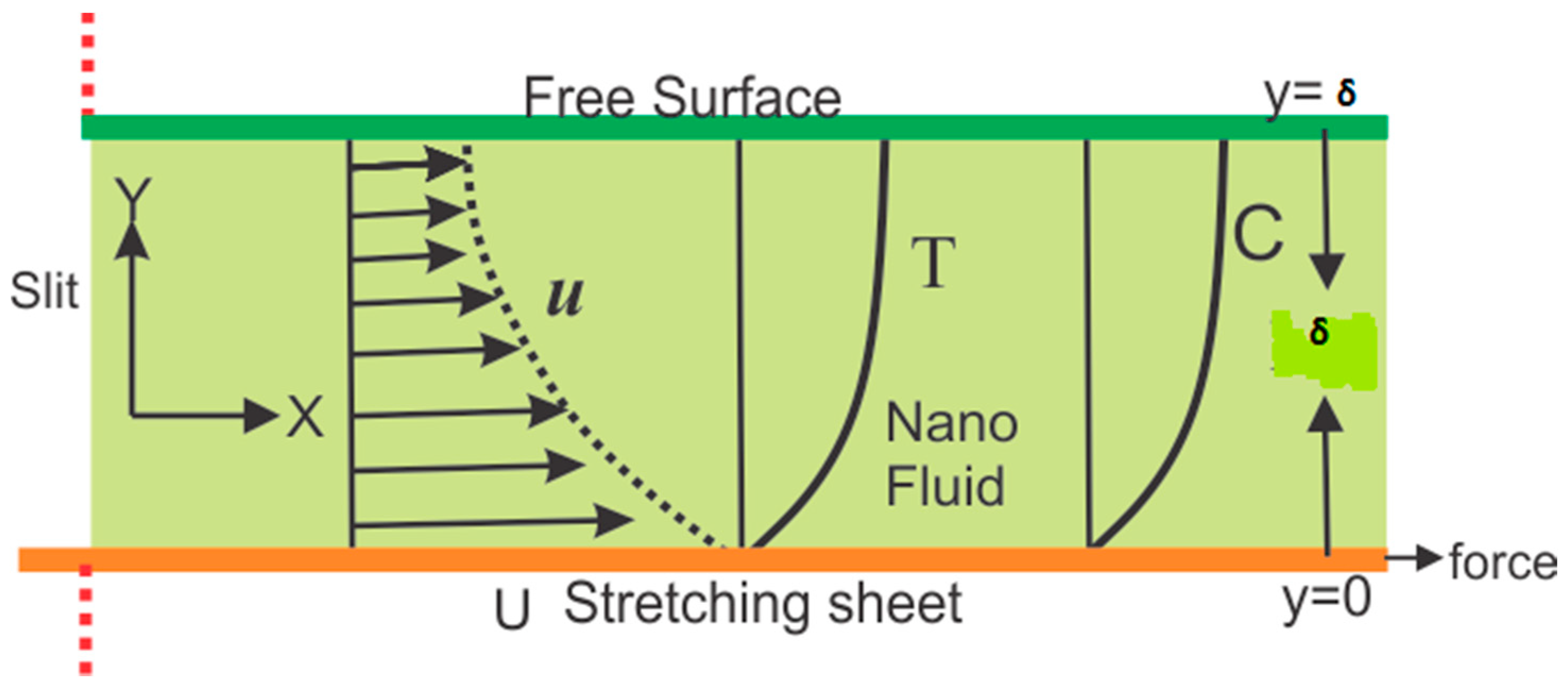
Thin Film Flow of Micropolar Fluid in a Permeable Medium


Abstract
:1. Introduction
2. Mathematical Formulation
3. Solution Methodology
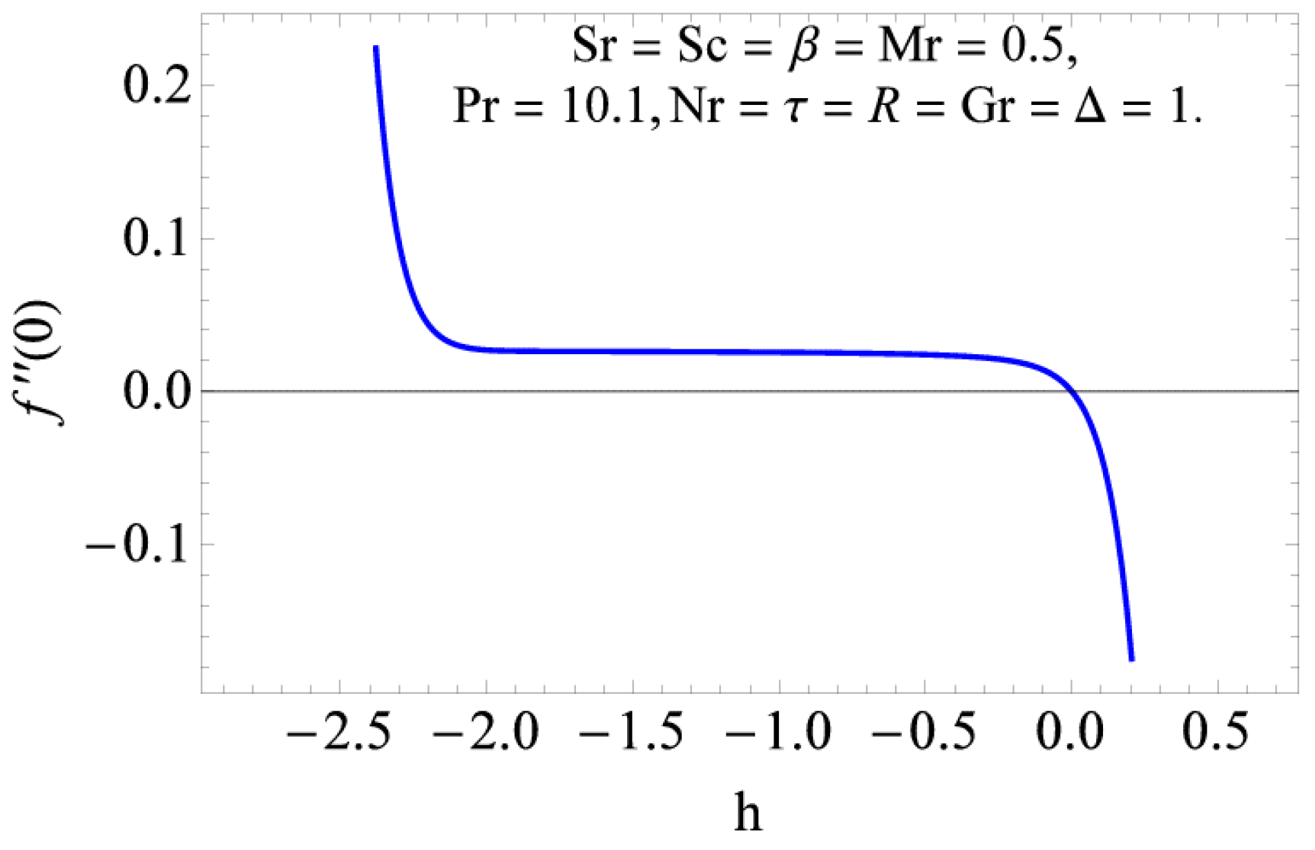
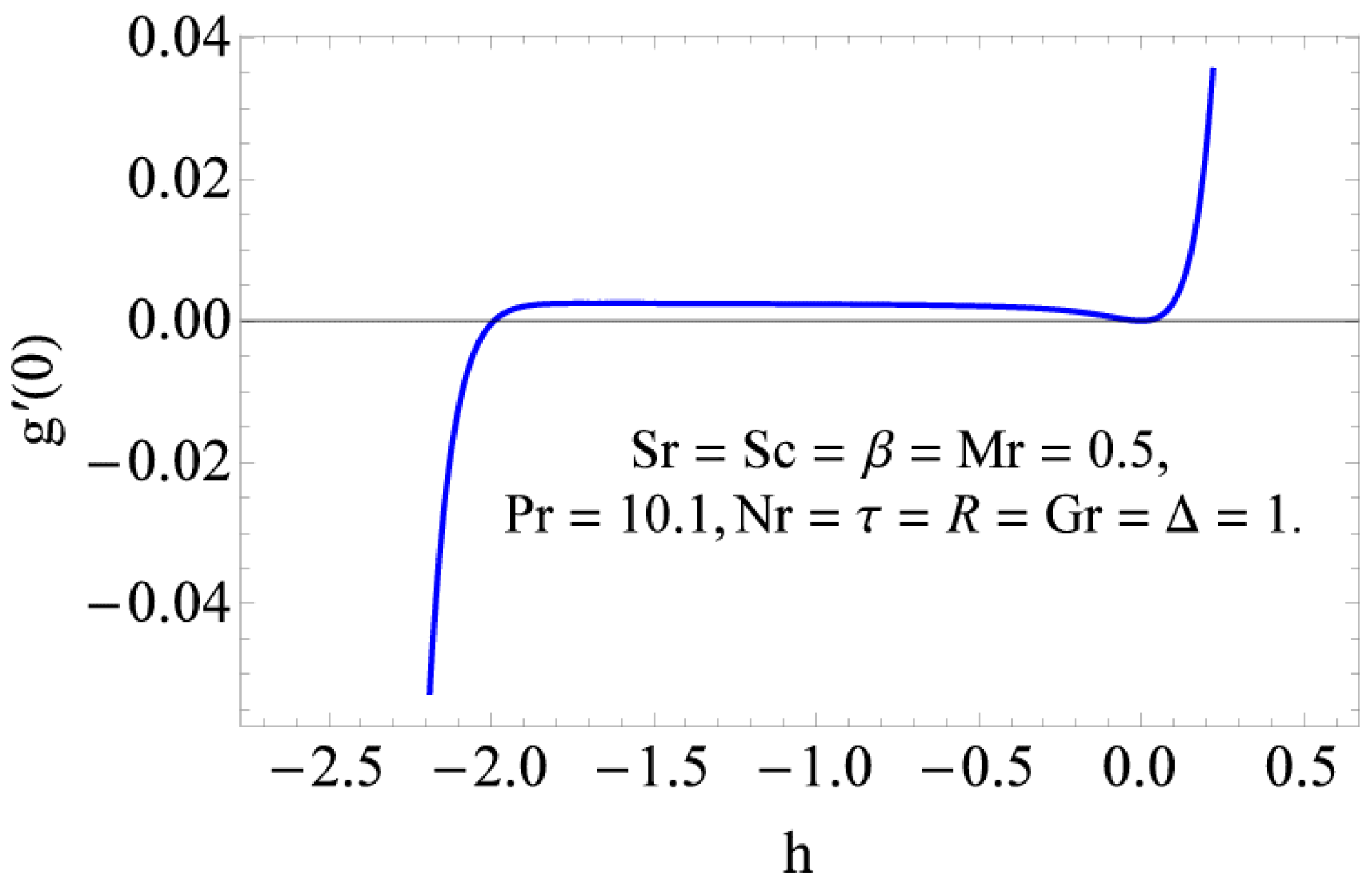
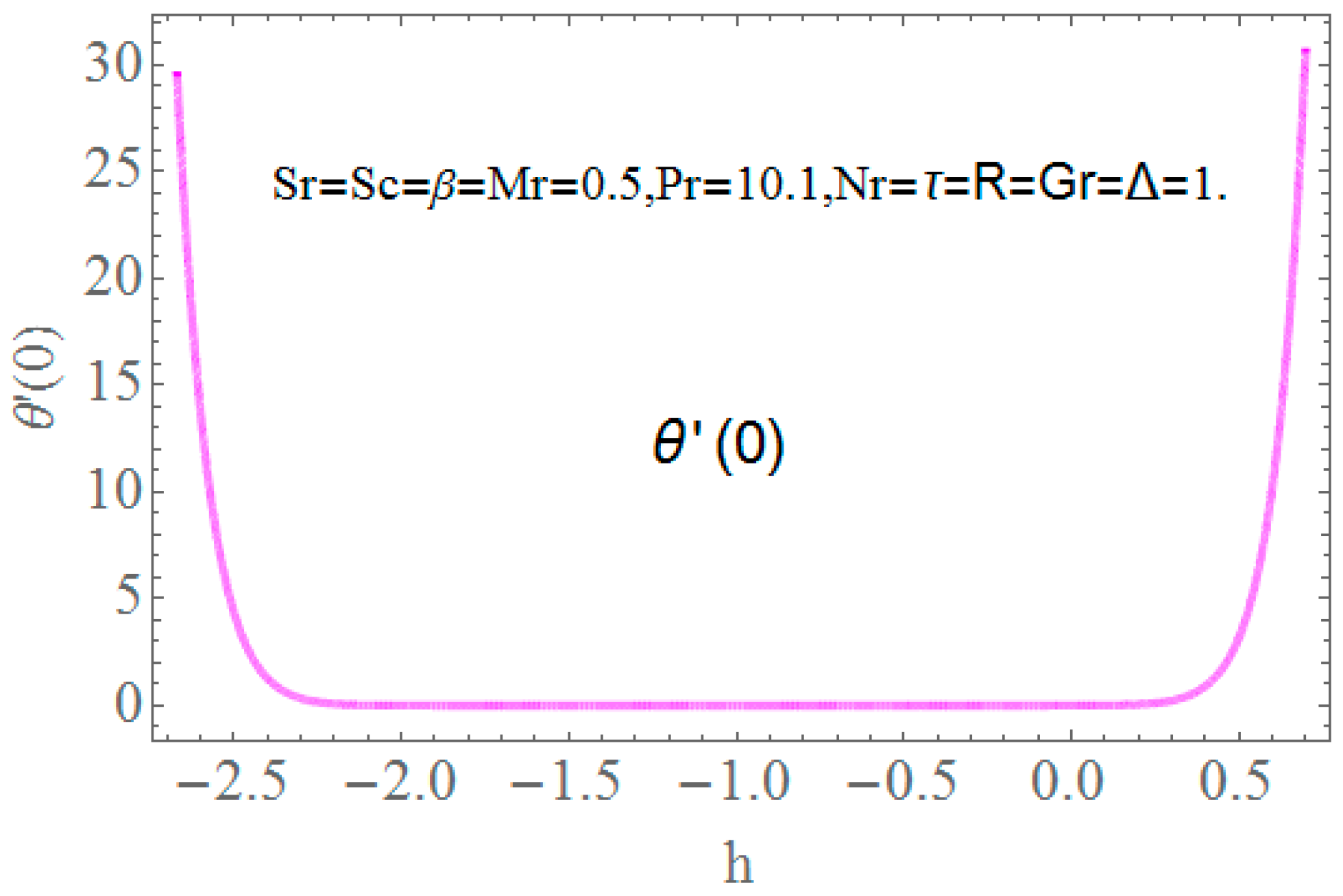
3.1. Homotopy Analysis Method
3.2. Numerical Solution
4. Graphical Results and Discussion
5. Conclusions
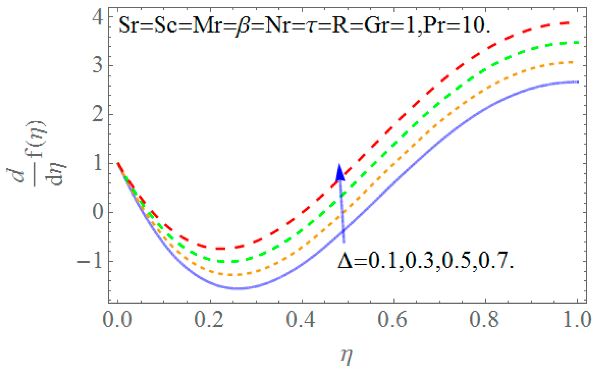
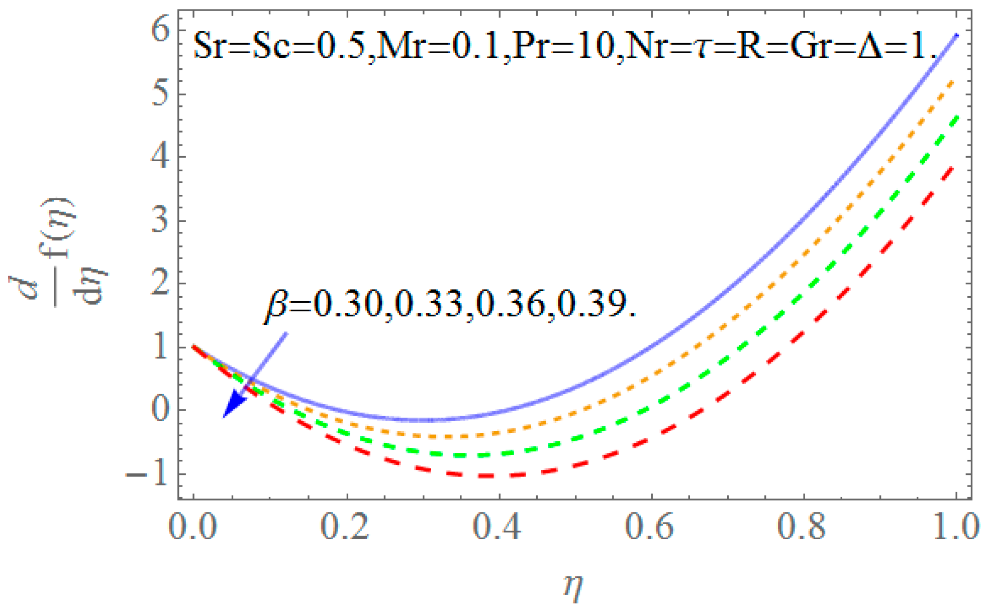
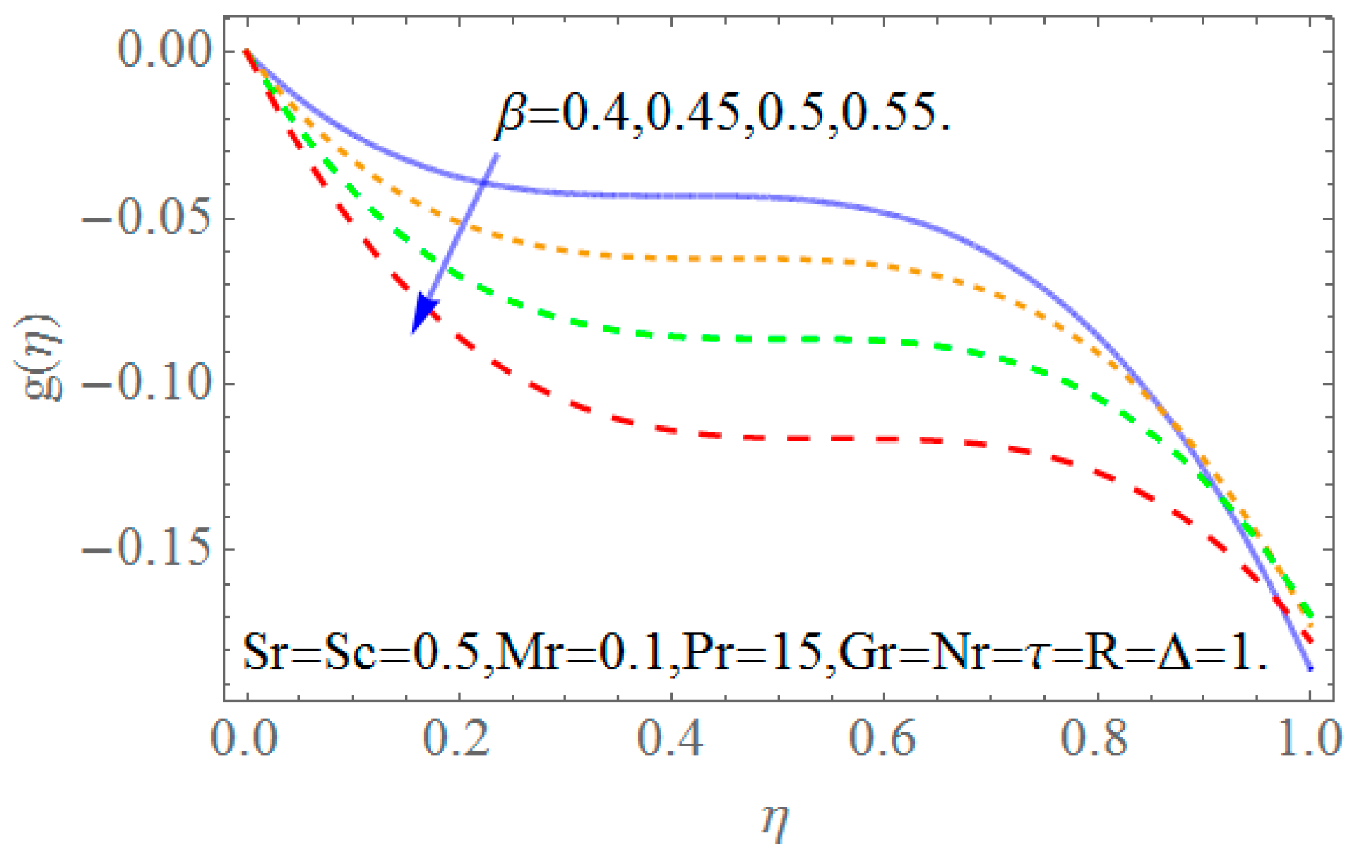
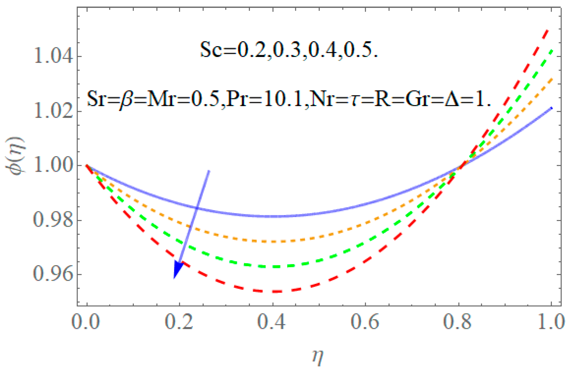
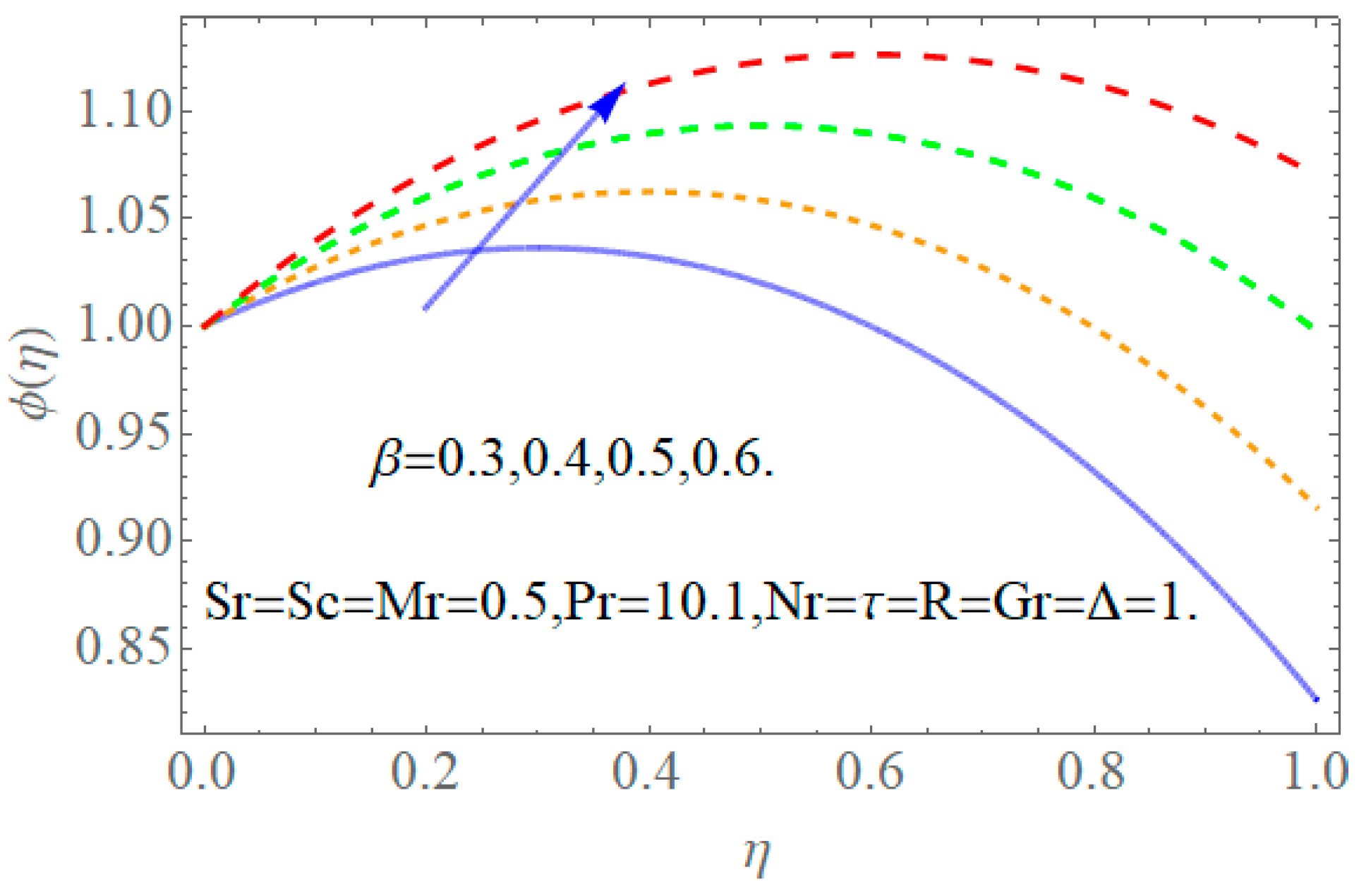
- The increasing values of the thin film thickness parameter improve the resistance force to decline the velocity and microrotation profiles, and enhance the concentration field.
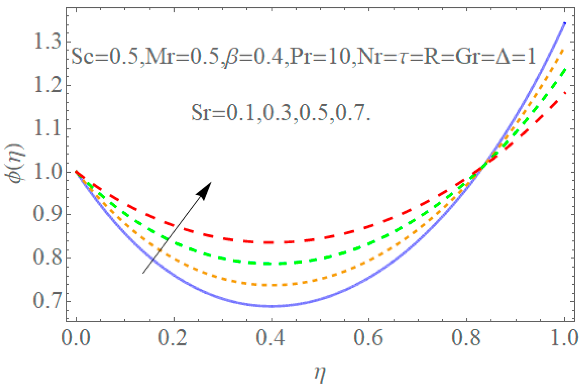
- It was observed that the rise in the Soret number enhances the concentration field .
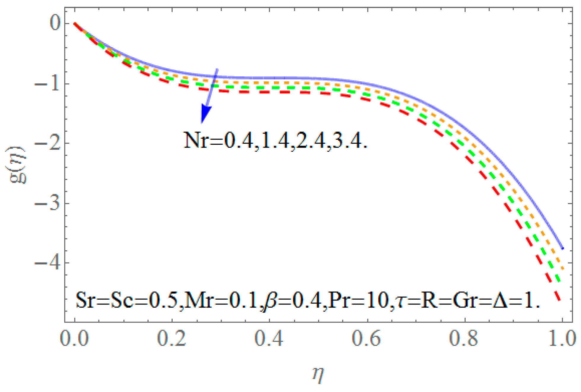
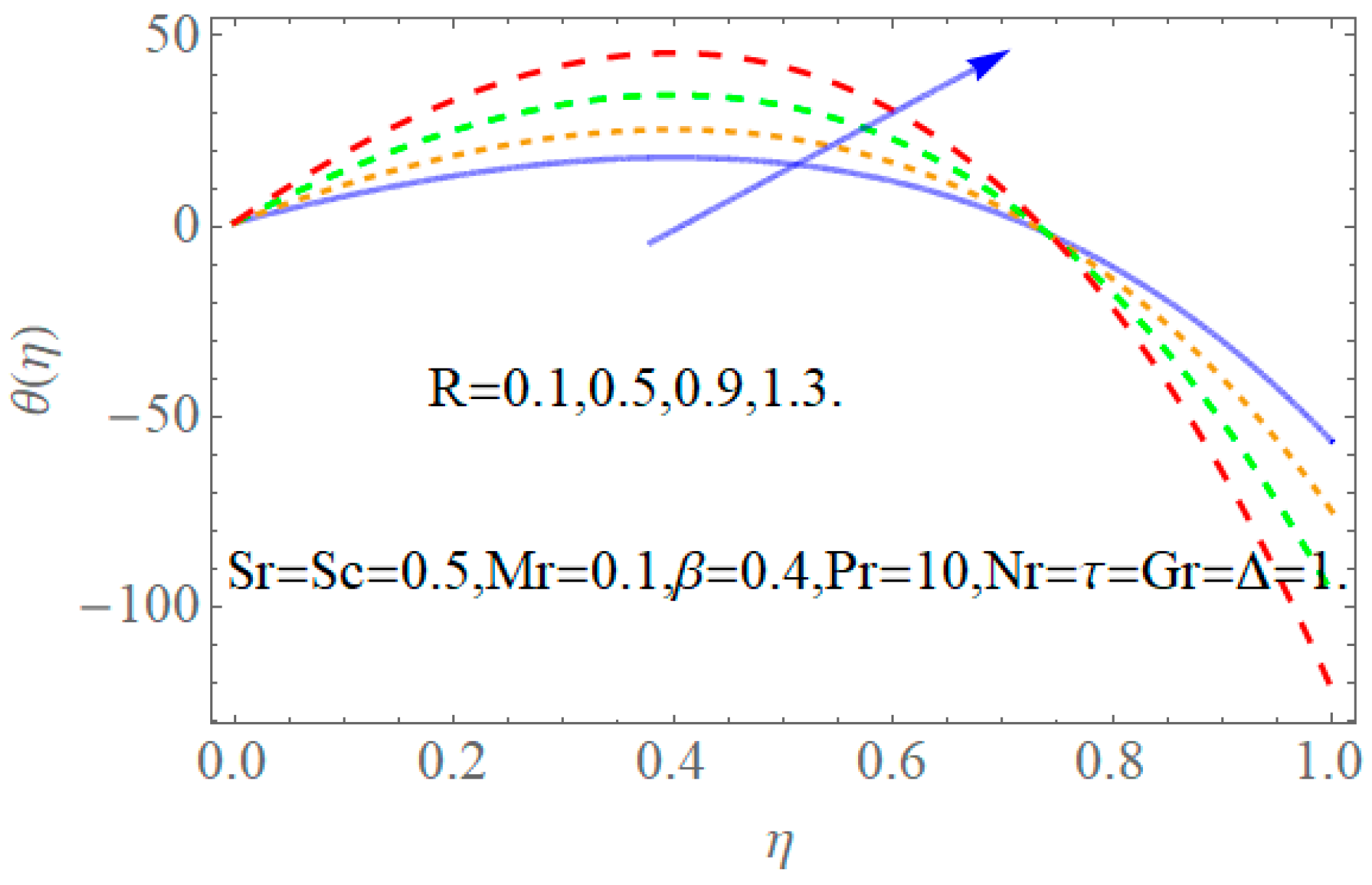
- The temperature field rises with the increasing value of the thermal radiation parameter because of the rate of energy and transport growth, and consequently enhances the temperature profile.
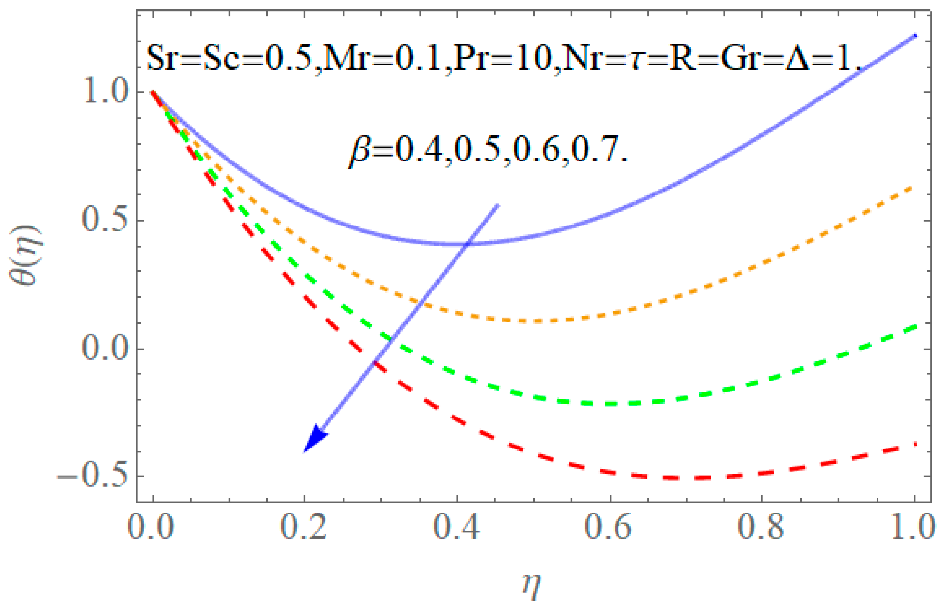
- The increase in the thickness of the thin film reduces the temperature profile. Physically, heat transfer is larger in the thin film as compared with the thick film, while the concentration field increases as the thin film parameter increases.
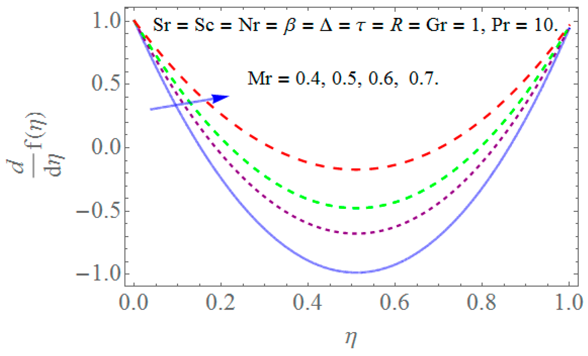
- The larger vortex–viscosity parameter causes the velocity of the liquid film to rise.
- The HAM solution was validated with the numerical solution (ND-solve) and very close agreement was observed.
Author Contributions
Funding
Conflicts of Interest
Nomenclature
| Cartesian coordinates | |
| Velocity components | |
| Stretching velocity | |
| Uniform thickness of the thin film | |
| Wall temperature field | |
| Surface concentration | |
| Reference temperature | |
| Reference concentration | |
| Kinematic viscosity | |
| Dynamic viscosity | |
| constant characteristic | |
| Forchheimer inertia constant | |
| coupling constant | |
| Temperature field | |
| Concentration field | |
| Fluid density | |
| Liquid film thickness | |
| Radiative heat fluctuation | |
| Stefan–Boltzmann constant | |
| Concentration molecular diffusivity | |
| Mean temperature | |
| permeability | |
| Stream function | |
| Non-dimensional thickness of the Nano liquid film | |
| porosity parameter | |
| Prandtl number | |
| Schmidt number | |
| Soret number | |
| is the microrotation constant | |
| Thermal radiation parameter | |
| Thermophoretic velocity |
References
- Goldsmith, P.; May, F.G. Diffusiophoresis and Thermophoresis in Water Vapour Systems; Aerosol Science, Academic Press: London, UK, 1966; pp. 163–194. [Google Scholar]
- Goren, S.L. Thermophoresis of aerosol particles in the laminar boundary layer on a flat plate. J. Colloid Interface Sci. 1977, 61, 77–85. [Google Scholar] [CrossRef]
- Jayaraj, S.; Dinesh, K.K.; Pillai, K.L. Thermophoresis in natural convection with variable properties. Heat Mass Transf. 1999, 34, 469–475. [Google Scholar] [CrossRef]
- Selim, A.; Hossain, M.A.; Rees, D.A.S. The effect of surface mass transfer on mixed convection flow past a heated vertical flat permeable plate with thermophoresis. Int. J. Therm. Sci. 2003, 42, 973–982. [Google Scholar] [CrossRef]
- Chamkha, A.J.; Pop, I. Effect of thermophoresis particle deposition in free convection boundary layer from a vertical flat plate embedded in a porous medium. Int. Commun. Heat Mass Transf. 2004, 31, 421–430. [Google Scholar] [CrossRef]
- Chamkha, A.J.; Al-Mudhaf, A.F.; Pop, I. Effect of heat generation or absorption on thermophoretic free convection boundary layer from a vertical flat plate embedded in a porous medium. Int. Commun. Heat Mass Transf. 2006, 33, 1096–1102. [Google Scholar] [CrossRef]
- Das, K. Impact of thermal radiation on MHD slip flow over a flat plate with variable fluid properties. Heat Mass Transf. 2012, 48, 767–778. [Google Scholar] [CrossRef]
- Al-Hadhrami, A.K.; Elliott, L.; Ingham, D.B. A new model for viscous dissipation in a porous media across a range of permeability values. Transp. Porous Media 2003, 53, 117–122. [Google Scholar] [CrossRef]
- Al-Hadhrami, A.K.; Elliott, L.; Ingham, D.B. Combined free and forced convection in vertical channels of porous media. Transp. Porous Media 2002, 49, 265–289. [Google Scholar] [CrossRef]
- Łukaszewicz, G. Micropolar Fluids: Theory and Application; Birkhauser: Basel, Switzerland, 1999. [Google Scholar]
- Aouadi, M. Numerical study for micropolar flow over a stretching sheet. Comput. Mater. Sci. 2007, 38, 774–780. [Google Scholar] [CrossRef]
- Chauhan, D.S.; Olkha, A. Slip flow and heat transfer of a second-grade fluid in a porous medium over a stretching sheet with power-law surface temperature or heat flux. Chem. Eng. Commun. 2011, 198, 1129–1145. [Google Scholar] [CrossRef]
- Cortell, R. Similarity solutions for flow and heat transfer of a viscoelastic fluid over a stretching sheet. Int. J. Non-Linear Mech. 1994, 29, 155–161. [Google Scholar] [CrossRef]
- Dandapat, B.S.; Gupta, A.S. Flow and heat transfer in a viscoelastic fluid over a stretching sheet. Int. J. Non-Linear Mech. 1989, 24, 215–219. [Google Scholar] [CrossRef]
- Chauhan, D.S.; Kumar, V. Unsteady flow of a non-Newtonian second grade fluid in a channel partially filled by a porous medium. Adv. Appl. Sci. Res. 2012, 3, 75–94. [Google Scholar]
- Khan, I.; Shafie, S. Rotating MHD flow of a generalized burgers’ fluid over an oscillating plate embedded in a porous medium. Therm. Sci. 2015, 19, 183–190. [Google Scholar] [CrossRef]
- Abo-Eldahab, E.M.; Ghonaim, A.F. Radiation effect on heat transfer of a micropolar fluid through a porous medium. Appl. Math. Comput. 2005, 169, 500–510. [Google Scholar] [CrossRef]
- Rashidi, M.M.; Pour, S.M. A novel analytical solution of heat transfer of a micropolar fluid through a porous medium with radiation by DTM-Padé. Heat Transf. Asian Res. 2010, 39, 575–589. [Google Scholar] [CrossRef]
- Rashidi, M.M.; Abbasbandy, S. Analytic approximate solutions for heat transfer of a micropolar fluid through a porous medium with radiation. Commun. Nonlinear Sci. Numer. Simul. 2011, 16, 1874–1889. [Google Scholar] [CrossRef]
- Heydari, M.; Loghmani, G.B.; Hosseini, S.M. Exponential bernstein functions: An effective tool for the solution of heat transfer of a micropolar fluid through a porous medium with radiation. Comput. Appl. Math. 2017, 36, 647–675. [Google Scholar] [CrossRef]
- Tripathy, R.S.; Dash, G.C.; Mishra, S.R.; Hoque, M.M. Numerical analysis of hydromagnetic micropolar fluid along a stretching sheet embedded in porous medium with non-uniform heat source and chemical reaction. Eng. Sci. Technol. Int. J. 2016, 19, 1573–1581. [Google Scholar] [CrossRef] [Green Version]
- Rahman, M.M.; Sattar, M.A. MHD free convection and mass transfer flow with oscillatory plate velocity and constant heat source in a rotating frame of reference. Dhaka Univ. J. Sci. 1999, 47, 63–73. [Google Scholar]
- Bakr, A.A. Effects of chemical reaction on MHD free convection and mass transfer flow of a micropolar fluid with oscillatory plate velocity and constant heat source in a rotating frame of reference. Commun. Nonlinear Sci. Numer. Simulat. 2011, 16, 698–710. [Google Scholar] [CrossRef]
- Ramzan, M.; Ullah, N.; Chung, J.D.; Lu, D.; Farooq, U. Buoyancy effects on the radiative magneto Micropolar nanofluid flow with double stratification, activation energy and binary chemical reaction. Sci. Rep. 2017, 7, 12901. [Google Scholar] [CrossRef] [PubMed] [Green Version]
- Srinivasacharya, D.; Ramreddy, C. Natural convection heat and mass transfer in a micropolar fluid with thermal and mass stratification. Int. J. Comput. Methods Eng. Sci. Mech. 2013, 14, 401–413. [Google Scholar] [CrossRef]
- Nadeem, S.; Hussain, S.T. Flow and heat transfer analysis of Williamson nanofluid. Appl. Nanosci. 2014, 4, 1005–1012. [Google Scholar] [CrossRef]
- Khan, W.; Gul, T.; Idrees, M.; Islam, S.; Khan, I.; Dennis, L.C.C. Thin film williamson nanofluid flow with varying viscosity and thermal conductivity on a time-dependent stretching sheet. Appl. Sci. 2016, 6, 334. [Google Scholar] [CrossRef]
- Aziz, R.C.; Hashim, I.; Alomari, A.K. Thin film flow and heat transfer on an unsteady stretching sheet with internal heating. Meccanica 2011, 46, 349–357. [Google Scholar] [CrossRef]
- Qasim, M.; Khan, Z.H.; Lopez, R.J.; Khan, W.A. Heat and mass transfer in nanofluid thin film over an unsteady stretching sheet using Buongiorno’s model. Eur. Phys. J. Plus 2016, 131, 16. [Google Scholar] [CrossRef]
- Tawade, J.; Abel, M.S.; Metri, P.G.; Koti, A. Thin film flow and heat transfer over an unsteady stretching sheet with thermal radiation, internal heating in presence of external magnetic field. Int. J. Adv. Appl. Math. Mech. 2016, 3, 29–40. [Google Scholar]
- Khan, Y.; Wu, Q.; Faraz, N.; Yildirim, A. The effects of variable viscosity and thermal conductivity on a thin film flow over a shrinking/stretching sheet. Comput. Math. Appl. 2011, 61, 3391–3399. [Google Scholar] [CrossRef] [Green Version]
- Mahmood, T.; Khan, N. Thin film flow of a third grade fluid through porous medium over an inclined plane. Int. J. Nonlinear Sci. 2012, 14, 53–59. [Google Scholar]
- Shijun, L. Homotopy analysis method: A new analytic method for nonlinear problems. Appl. Math. Mech. 1998, 19, 957–962. [Google Scholar] [CrossRef]
- Liao, S. On the homotopy analysis method for nonlinear problems. Appl. Math. Comput. 2004, 147, 499–513. [Google Scholar] [CrossRef]
- Liao, S. Homotopy Analysis Method in Nonlinear Differential Equations; Higher Education Press: Beijing, China, 2012; pp. 153–165. [Google Scholar]
- Gul, T.; Haleem, I.; Ullah, I.; Khan, M.A.; Bonyah, B.; Khan, I.; Shuaib, M. The study of the entropy generation in a thin film flow with variable fluid properties past over a stretching sheet. Adv. Mech. Eng. 2018, 10, 1–15. [Google Scholar] [CrossRef]
- Gul, T.; Nasir, S.; Islam, S.; Shah, Z.; Khan, M.A. Effective prandtl number model influences on the γAl2O3-H2O and γAl2O3-C2H6O2 nanofluids spray along a stretching cylinder. Arab. J. Sci. Eng. 2019, 2, 1601–1616. [Google Scholar] [CrossRef]


| 0.3 | 0.8 | 0.3 | 1.36594 |
| 0.4 | 0.8 | 0.3 | 1.36571 |
| 0.5 | 0.8 | 0.3 | 1.36547 |
| 0.3 | 0.8 | 0.3 | 1.36594 |
| 0.3 | 0.9 | 0.3 | 1.24938 |
| 0.3 | 1.0 | 0.3 | 1.15533 |
| 0.3 | 0.8 | 0.3 | 1.36594 |
| 0.3 | 0.8 | 0.4 | 1.45338 |
| 0.3 | 0.8 | 0.5 | 1.54067 |
| 0.3 | 0.3 | 0.246741 |
| 0.4 | 0.3 | 0.240841 |
| 0.5 | 0.3 | 0.235105 |
| 0.3 | 0.3 | 0.246741 |
| 0.3 | 0.4 | 0.325885 |
| 0.3 | 0.5 | 0.403524 |
| 0.3 | 0.3 | 0.3 | 0.265463 |
| 0.4 | 0.3 | 0.3 | 0.350588 |
| 0.5 | 0.3 | 0.3 | 0.434081 |
| 0.3 | 0.3 | 0.3 | 0.265463 |
| 0.3 | 0.4 | 0.3 | 0.264059 |
| 0.3 | 0.5 | 0.3 | 0.262655 |
| 0.3 | 0.3 | 0.3 | 0.265463 |
| 0.3 | 0.3 | 0.4 | 0.266868 |
| 0.3 | 0.3 | 0.5 | 0.268272 |
| Numerical Solution | Absolute Error | ||
|---|---|---|---|
| 0 | 0.000000 | ||
| 0.1 | 0.099999 | 0.100043 | |
| 0.2 | 0.199999 | 0.200168 | |
| 0.3 | 0.299999 | 0.300364 | |
| 0.4 | 0.399999 | 0.400624 | |
| 0.5 | 0.499999 | 0.500937 | |
| 0.6 | 0.599999 | 0.601295 | |
| 0.7 | 0.699999 | 0.701689 | |
| 0.8 | 0.799999 | 0.802110 | |
| 0.9 | 0.899999 | 0.902549 | |
| 1 | 0.999999 | 1.002997 |
| Numerical Solution | Absolute Error | ||
|---|---|---|---|
| 0 | −1.28767269 | −0.0000000 | |
| 0.1 | −0.0094987 | −0.0088208 | |
| 0.2 | −0.0167880 | −0.0157937 | |
| 0.3 | −0.0221826 | −0.0211439 | |
| 0.4 | −0.0259819 | −0.0250914 | |
| 0.5 | −0.0284720 | −0.0278531 | |
| 0.6 | −0.0299279 | −0.0296435 | |
| 0.7 | −0.0306156 | −0.0306741 | |
| 0.8 | −0.0307942 | −0.0311543 | |
| 0.9 | −0.0307176 | −0.0312916 | |
| 1 | −0.0306366 | −0.0312919 |
| Numerical Solution | Absolute Error | ||
|---|---|---|---|
| 0 | 0.999999989 | 1.000000 | |
| 0.1 | 0.924017 | 0.925128 | |
| 0.2 | 0.855763 | 0.857526 | |
| 0.3 | 0.795601 | 0.797495 | |
| 0.4 | 0.743742 | 0.745268 | |
| 0.5 | 0.700264 | 0.701015 | |
| 0.6 | 0.665136 | 0.664844 | |
| 0.7 | 0.638237 | 0.636805 | |
| 0.8 | 0.619370 | 0.616887 | |
| 0.9 | 0.608278 | 0.605027 | |
| 1 | 0.604656 | 0.601109 |
| Numerical Solution | Absolute Error | ||
|---|---|---|---|
| 0 | 1.000000091 | 1.000000 | |
| 0.1 | 0.898855 | 0.90411 | |
| 0.2 | 0.809875 | 0.81792 | |
| 0.3 | 0.733047 | 0.741694 | |
| 0.4 | 0.668142 | 0.675623 | |
| 0.5 | 0.614767 | 0.619828 | |
| 0.6 | 0.572423 | 0.57436 | |
| 0.7 | 0.540544 | 0.539208 | |
| 0.8 | 0.518529 | 0.514298 | |
| 0.9 | 0.505765 | 0.499496 | |
| 1 | 0.501644 | 0.494614 |
© 2019 by the authors. Licensee MDPI, Basel, Switzerland. This article is an open access article distributed under the terms and conditions of the Creative Commons Attribution (CC BY) license (http://creativecommons.org/licenses/by/4.0/).
Share and Cite
Ali, V.; Gul, T.; Afridi, S.; Ali, F.; Alharbi, S.O.; Khan, I. Thin Film Flow of Micropolar Fluid in a Permeable Medium. Coatings 2019, 9, 98. https://doi.org/10.3390/coatings9020098
Ali V, Gul T, Afridi S, Ali F, Alharbi SO, Khan I. Thin Film Flow of Micropolar Fluid in a Permeable Medium. Coatings. 2019; 9(2):98. https://doi.org/10.3390/coatings9020098
Chicago/Turabian StyleAli, Vakkar, Taza Gul, Shakeela Afridi, Farhad Ali, Sayer Obaid Alharbi, and Ilyas Khan. 2019. "Thin Film Flow of Micropolar Fluid in a Permeable Medium" Coatings 9, no. 2: 98. https://doi.org/10.3390/coatings9020098