Nanofluids Thin Film Flow of Reiner-Philippoff Fluid over an Unstable Stretching Surface with Brownian Motion and Thermophoresis Effects


Abstract
:1. Introduction:
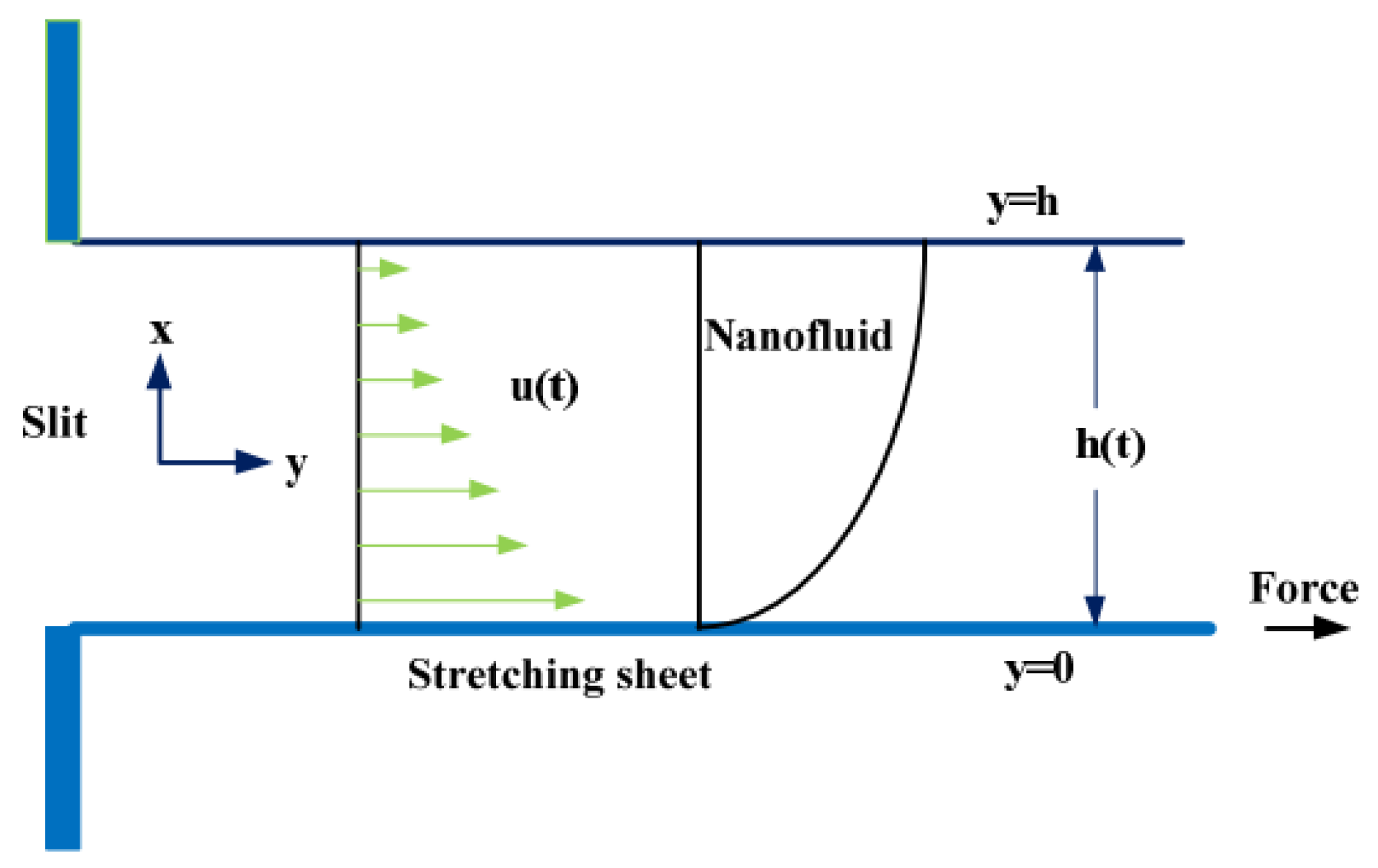
2. Problem Formulation
3. Solution by HAM
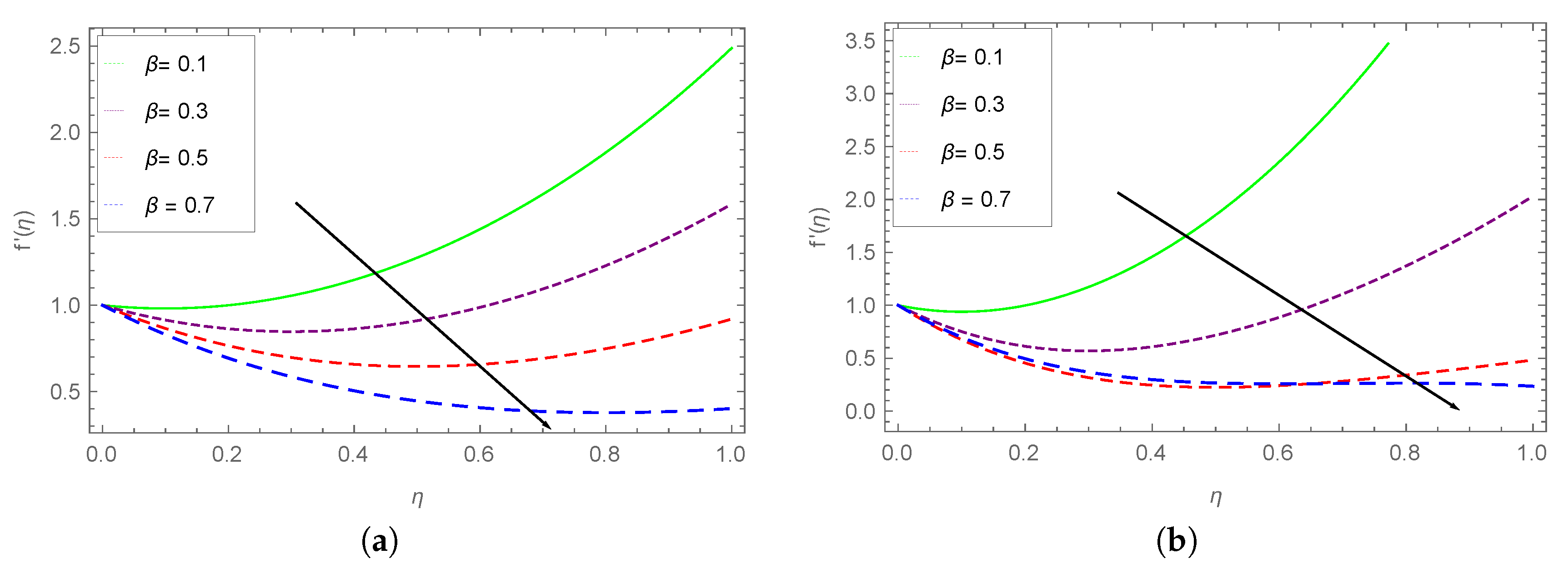
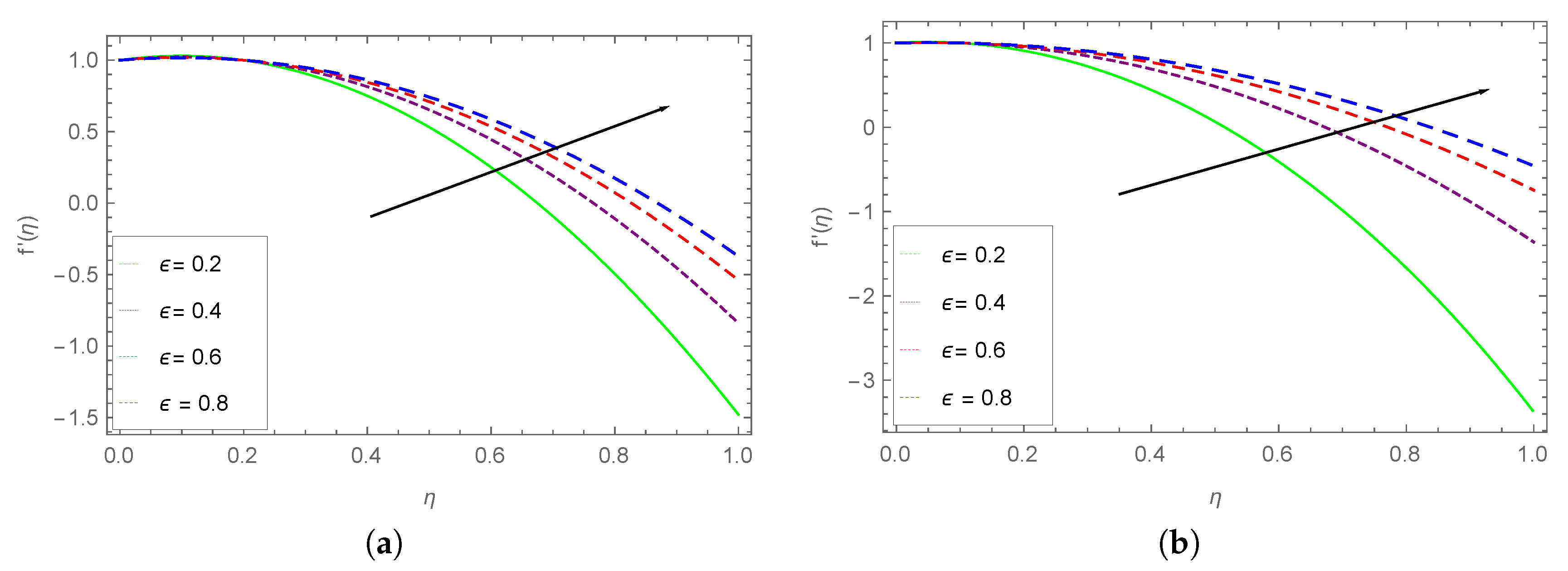
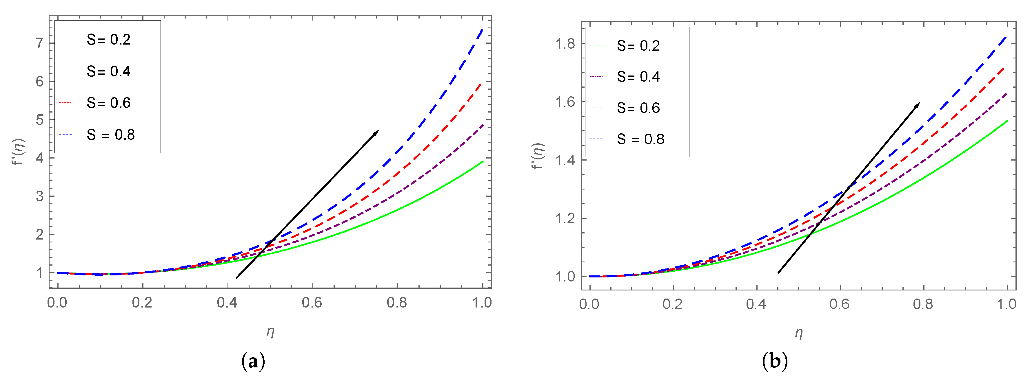
4. Results and Discussion
5. Tables Discussion
6. Conclusions
- A comparative analysis for the stretching and unsteadiness parameters for the gradient of the velocity is discussed to observe the sensitivity of these parameters.
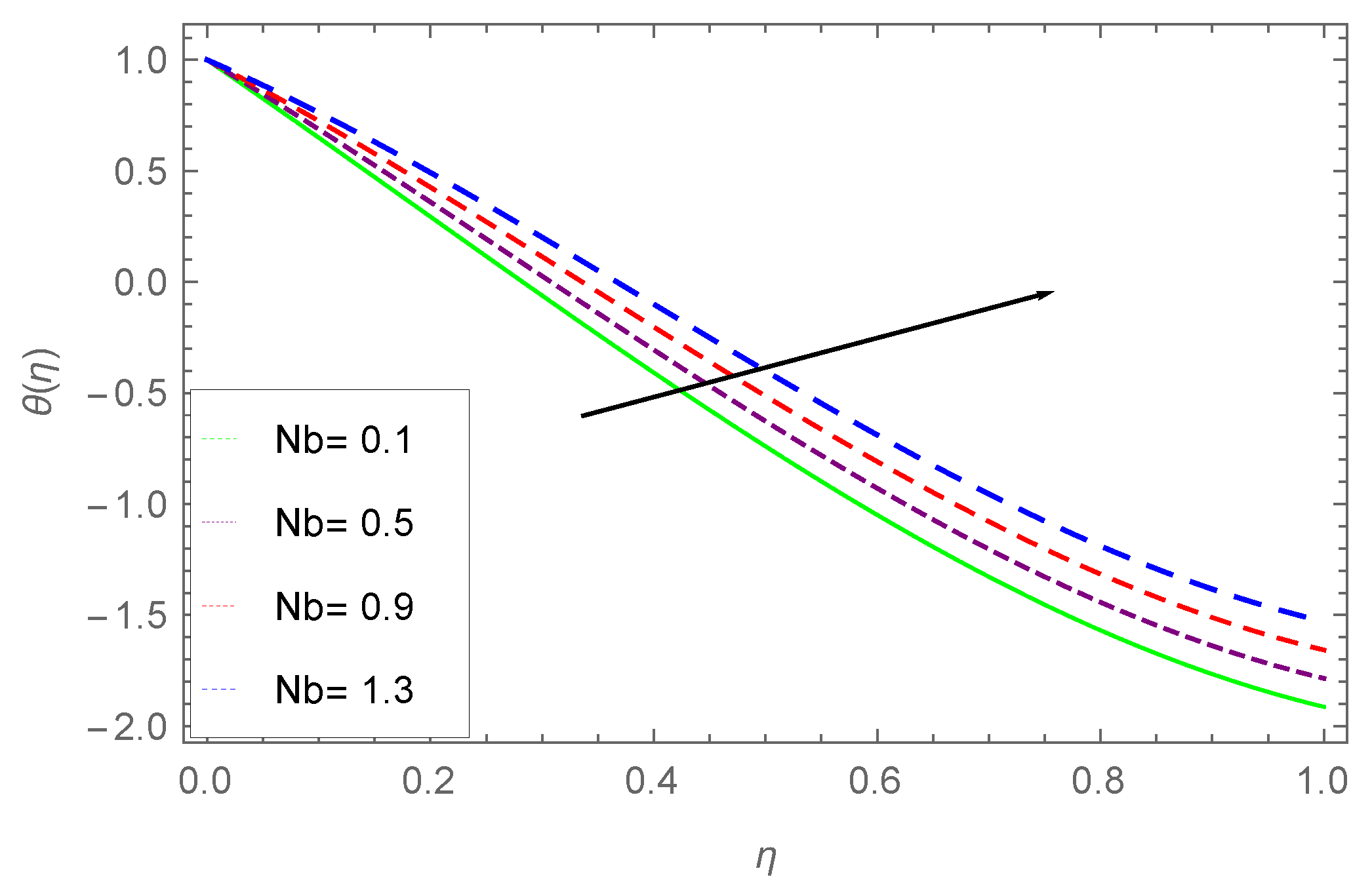
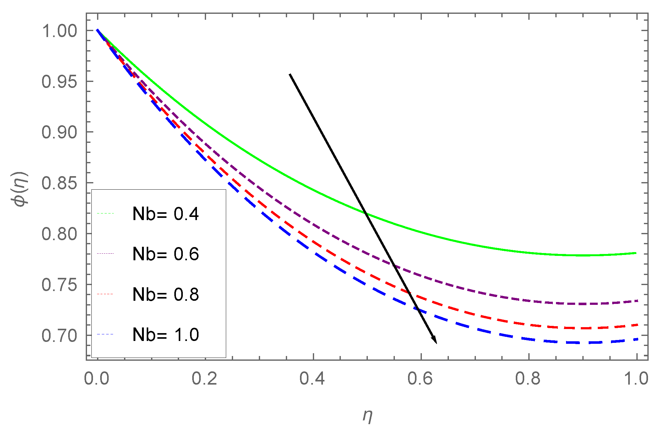
- The temperature profile climbs up with larger values of Brownian motion parameter .
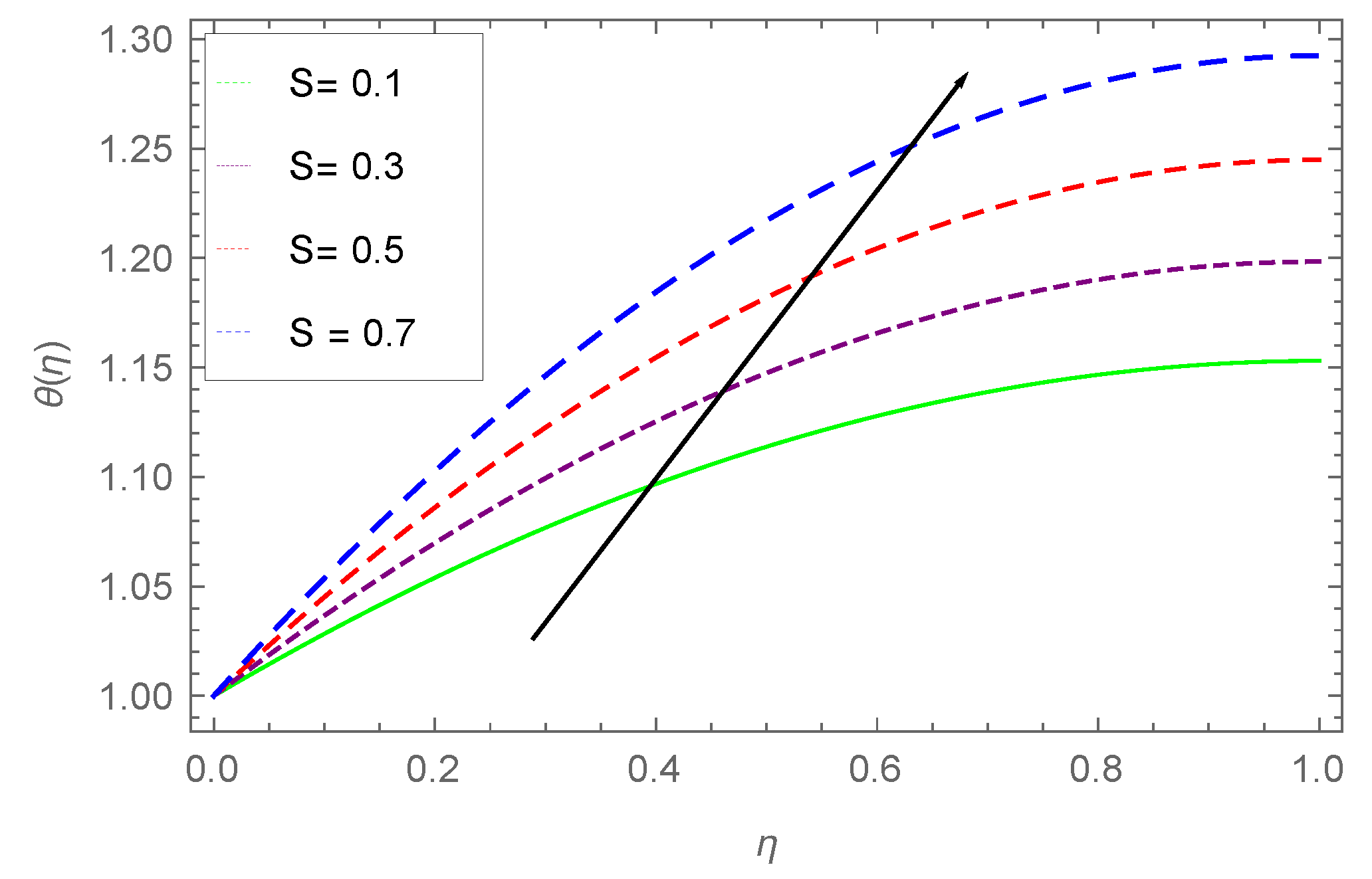
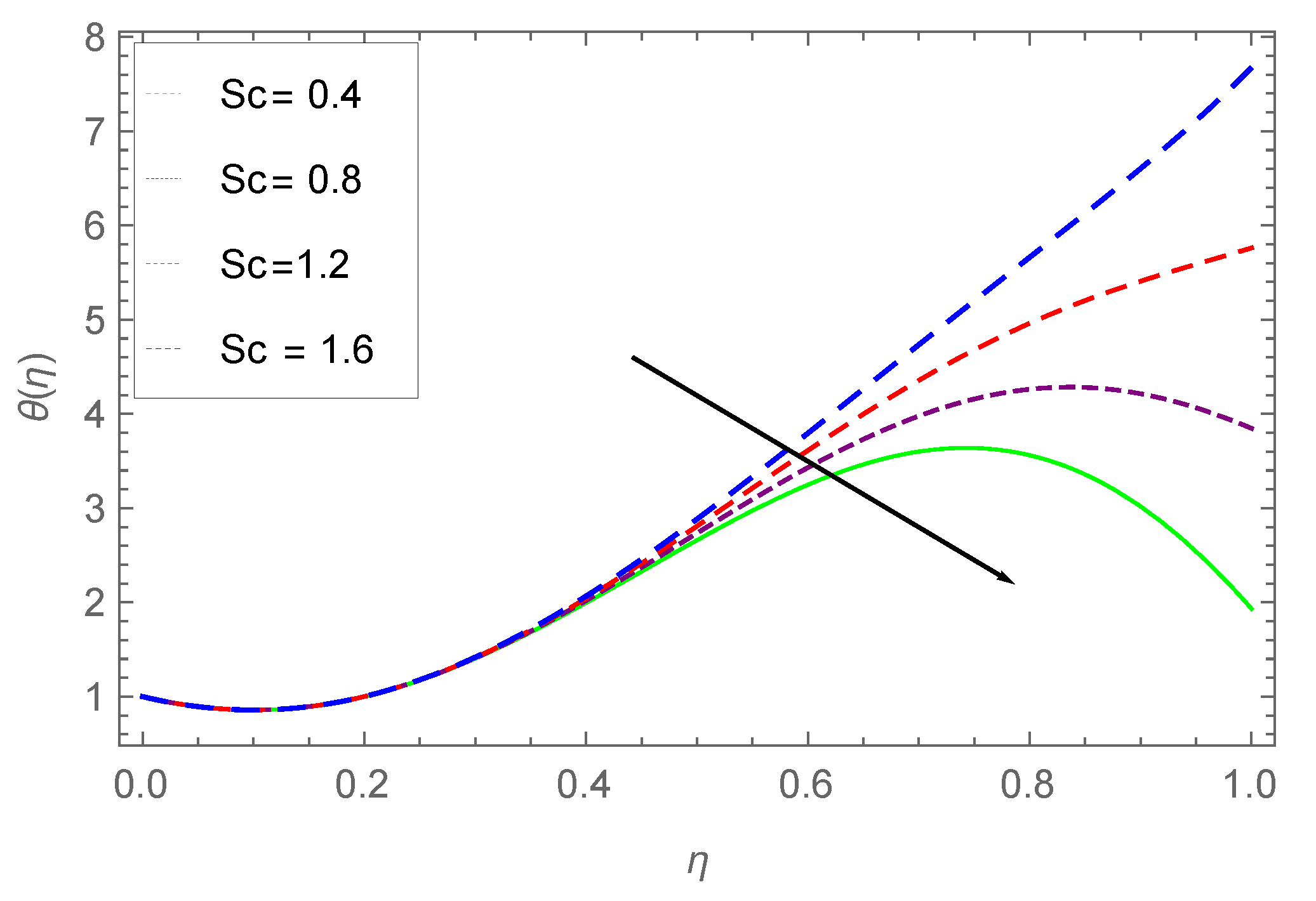
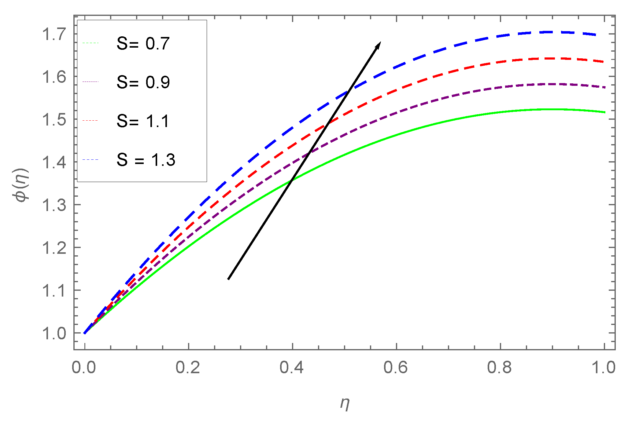
- Wth larger values of S, the thermal boundary layer thickness reduces.
- Higher values of increase the surface temperature, where an opposite effect is observed for unsteady parameter S, i.e., large values of S reduce the temperature of the surface.
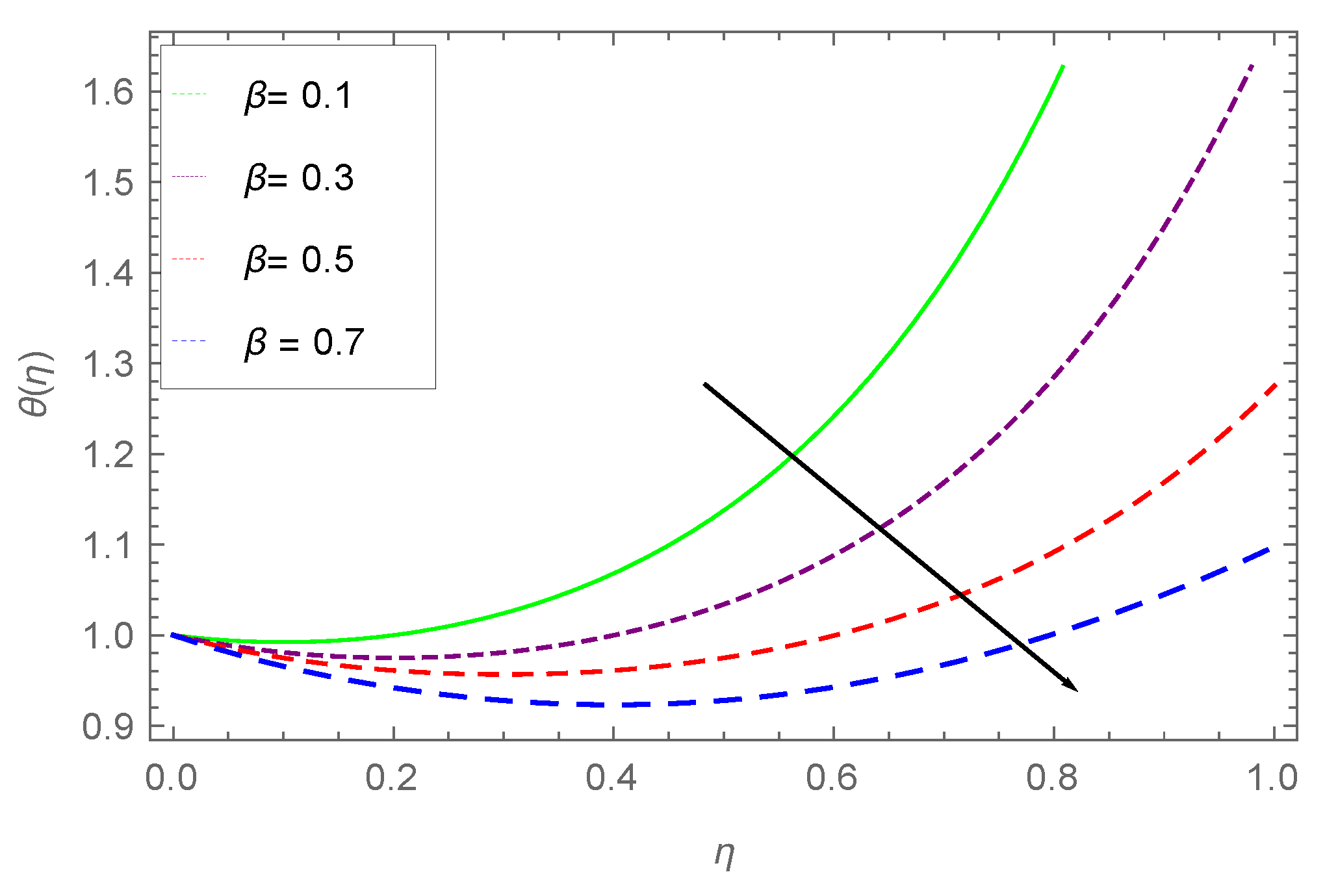
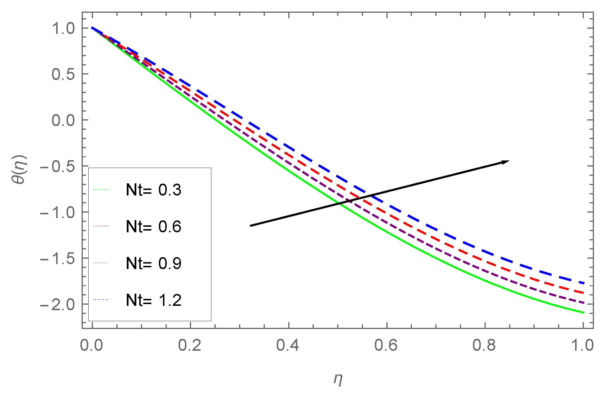
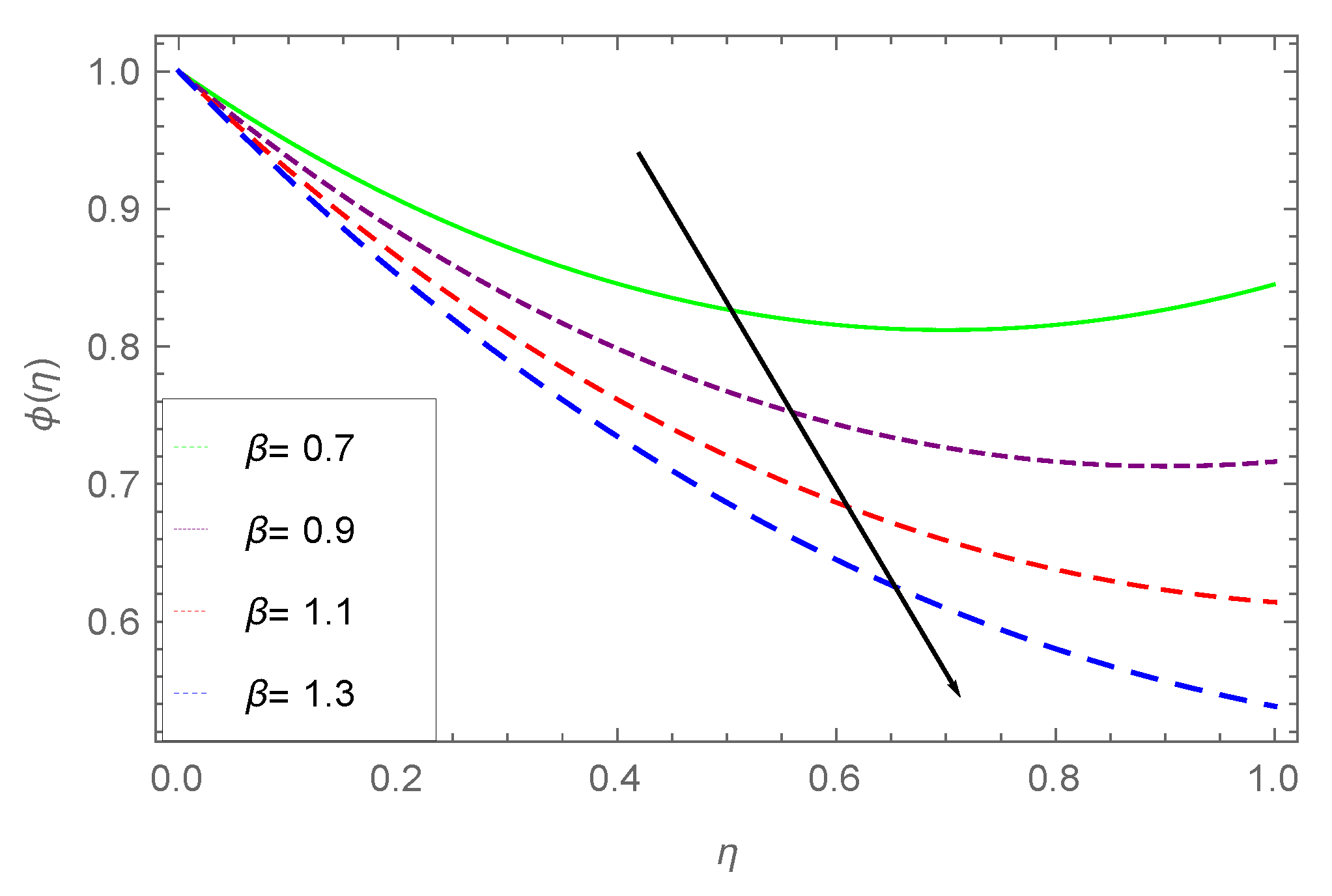
- It is examined that the heat profile decreases with increasing values of thermophoresis parameter , and increases with small numbers.
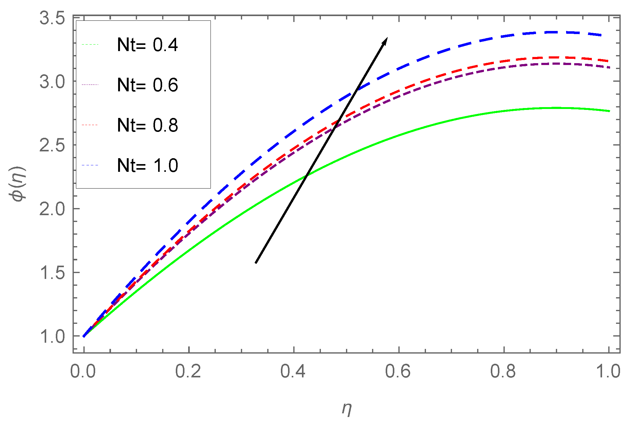
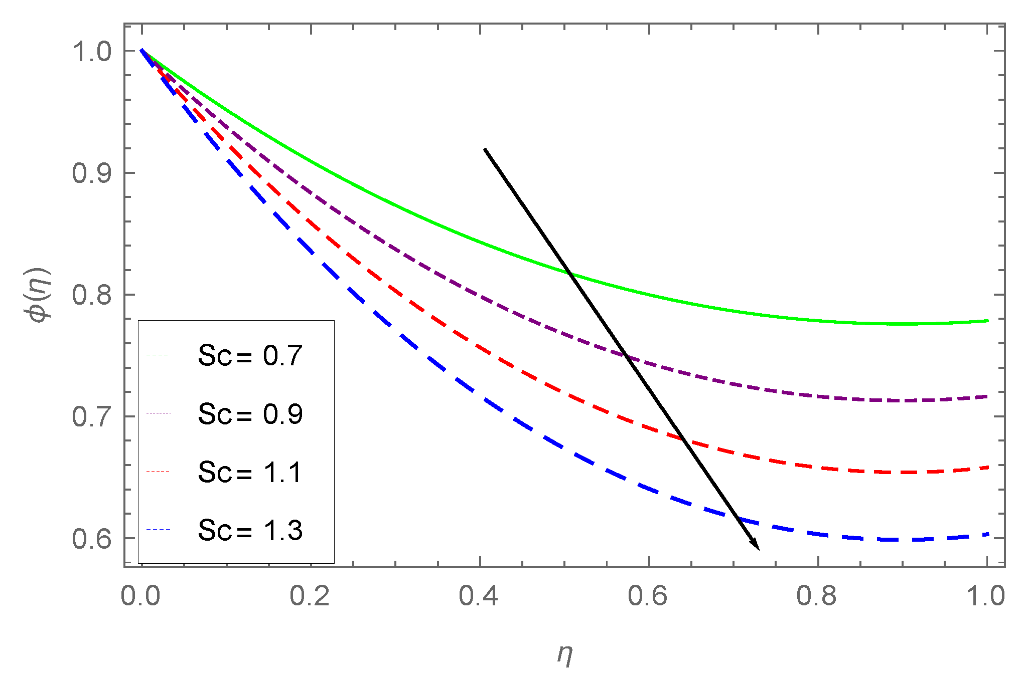
- The increasing values of reduce the mass flux, where increases the mass flux, while it rises with rising values of .
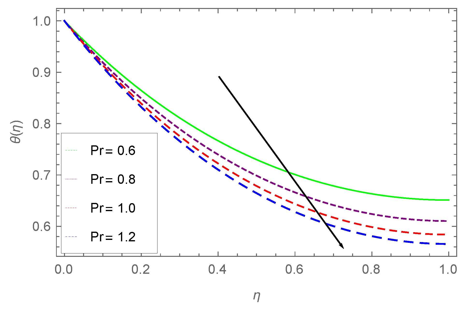
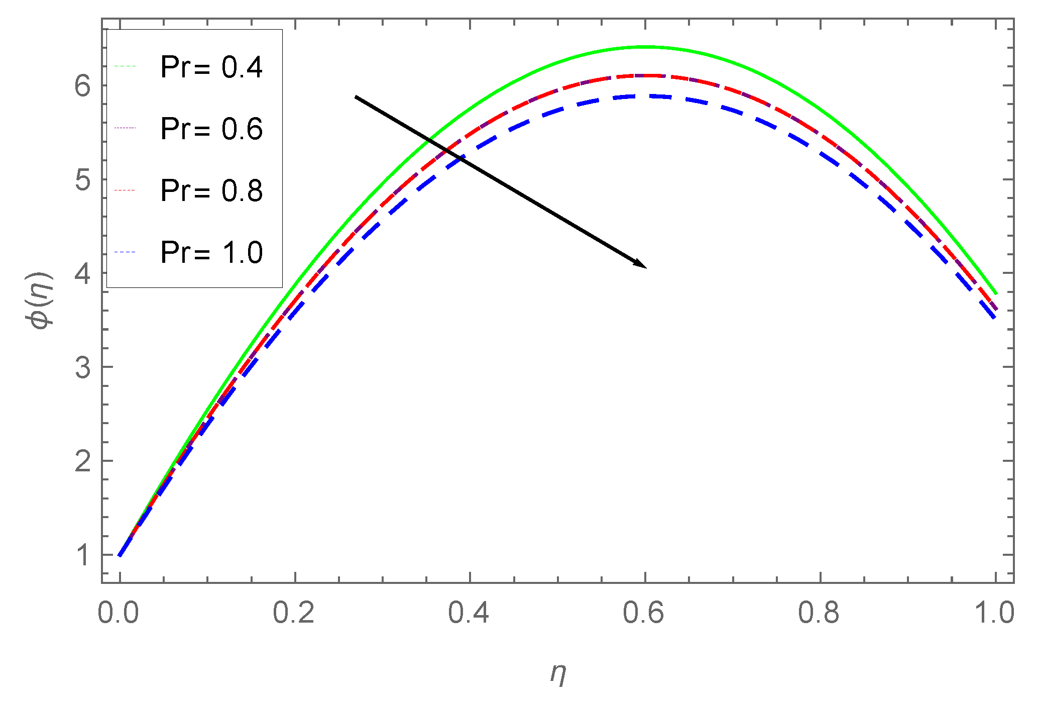
- The effect of Prandtl number on concentration and temperature profile is analyzed and a similar decline is observed in both the profiles.
- The convergence of the HAM method with the variation of the physical parameters is observed, and found its convergence more rapid as compared with other techniques.
Author Contributions
Acknowledgments
Conflicts of Interest
Abbreviations
| Sherhood number | |
| Film thickness parameter | |
| Nusslet number | |
| S | Unsteady parameter |
| Reynold number | |
| Prandtl number | |
| Stretching parameter | |
| Schmidth number | |
| Brownian diffusion of nanofluids | |
| Stretching velocity (m/s) | |
| Thermophoretic parameter | |
| Skin friction coefficient | |
| Brownian motion parameter | |
| Components of the strain rate | |
| Cauchy stress tensor | |
| T | Fluid temperature (K) |
| Extra stress tensor | |
| I | Identity tensor |
| Kinematic viscosity (m/s) | |
| Density (Kg/m) | |
| Dynamic viscosity (mPa) | |
| Specific heat (J K−1 g−1 K−1) | |
| Thermophoretic diffusion of nanofluids | |
| Thickness of liquid | |
| Absorption coefficient | |
| Heat Flux (W/m) | |
| Local Reynolds number | |
| Mass flux (K g s−1 m−2) | |
| f | Dimensionless velocity |
| ∞ | Condition at infinity |
| 0 | Reference condition |
| Velocity component in x-direction (m/s) | |
| Velocity component in y-direction (m/s) | |
| Coordinates (m) | |
| Similarity variable | |
| t | Time (s) |
References
- Bird, R.B.; Armstrong, R.C.; Hassager, O. Dynamics of Polymeric Liquids. Volume 1: Fluid Mechanics; John Wiley & Sons, Inc.: Hoboken, NJ, USA, 1987. [Google Scholar]
- Sakiadis, B.C. Boundary-layer behavior on continuous solid surfaces: I. Boundary-layer equations for two-dimensional and axisymmetric flow. AIChE J. 1961, 7, 26–28. [Google Scholar] [CrossRef]
- Crane, L.J. Flow past a stretching plate. J. Appl. Math. Phys. 1970, 21, 645–647. [Google Scholar] [CrossRef]
- Siddiqui, A.M.; Ahmed, M.; Ghori, Q.K. Thin film flow of non-Newtonian fluids on a moving belt. Chaos Solitons Fractals 2007, 33, 1006–1016. [Google Scholar] [CrossRef]
- Siddiqui, A.M.; Ashraf, A.; Azim, Q.A.; Babcock, B.S. Exact solutions for thin film flows of a PTT fluid down an inclined plane and on a vertically moving belt. Adv. Stud. Theor. Phys. 2013, 7, 65–87. [Google Scholar] [CrossRef]
- Tawade, J.; Abel, M.S.; Metri, P.G.; Koti, A. Thin film flow and heat transfer over an unsteady stretching sheet with thermal radiation, internal heating in presence of external magnetic field. Int. J. Adv. Appl. Math. Mech. 2016, 3, 29–40. [Google Scholar]
- Sajid, M.; Hayat, T.; Asghar, S. Comparison between the HAM and HPM solutions of thin film flows of non-Newtonian fluids on a moving belt. Nonlinear Dyn. 2007, 50, 27–35. [Google Scholar] [CrossRef]
- Bakier, A.Y. Thermal radiation effect on mixed convection from vertical surfaces in saturated porous media. Indian J. Pure Appl. Math. 2001, 32, 1157–1164. [Google Scholar] [CrossRef]
- Khan, N.; Mahmood, T. The influence of slip condition on the thin film flow of a third order fluid. Int. J. Nonlinear Sci. 2012, 13, 105–116. [Google Scholar]
- Moradi, A.; Ahmadikia, H.; Hayat, T.; Alsaedi, A. On mixed convection—Radiation interaction about an inclined plate through a porous medium. Int. J. Therm. Sci. 2013, 64, 129–136. [Google Scholar] [CrossRef]
- Chaudhary, S.; Singh, S.; Chaudhary, S. Thermal radiation effects on MHD boundary layer flow over an exponentially stretching surface. Appl. Math. 2015, 6, 295–303. [Google Scholar] [CrossRef]
- Eldabe, N.T.; Elsaka, A.G.; Radwan, A.E.; Eltaweel, M.A.M. Effects of chemical reaction and heat radiation on the MHD flow of visco-elastic fluid through a porous medium over a horizontal stretching flat plate. J. Am. Sci. 2010, 6, 126–135. [Google Scholar]
- Das, K. Effects of thermophoresis and thermal radiation on MHD mixed convective heat and mass transfer flow. Afr. Mat. 2013, 24, 511–524. [Google Scholar] [CrossRef]
- Hsiao, K.-L. Combined electrical MHD heat transfer thermal extrusion system using Maxwell fluid with radiative and viscous dissipation effects. Appl. Therm. Eng. 2017, 112, 1281–1288. [Google Scholar] [CrossRef]
- Hayat, T.; Sajjad, R.; Muhammad, T.; Alsaedi, A.; Ellahi, R. On MHD nonlinear stretching flow of Powell–Eyring nanomaterial. Results Phys. 2017, 7, 535–543. [Google Scholar] [CrossRef]
- Tian, X.; Li, B.; Hu, Z. Convective stagnation point flow of a MHD non-Newtonian nanofluid towards a stretching plate. Int. J. Heat Mass Transf. 2018, 127, 768–780. [Google Scholar] [CrossRef]
- Hsiao, K.-L. Micropolar nanofluid flow with MHD and viscous dissipation effects towards a stretching sheet with multimedia feature. Int. J. Heat Mass Transf. 2017, 112, 983–990. [Google Scholar] [CrossRef]
- Dandapat, B.S.; Gupta, A.S. Flow and heat transfer in a viscoelastic fluid over a stretching sheet. Int. J. Non-Linear Mech. 1989, 24, 215–219. [Google Scholar] [CrossRef]
- Wang, C. Liquid film on an unsteady stretching surface. Quart. Appl. Math. 1990, 48, 601–610. [Google Scholar] [CrossRef] [Green Version]
- Usha, R.; Sridharan, R. The axisymmetric motion of a liquid film on an unsteady stretching surface. J. Fluids Eng. 1995, 117, 81–85. [Google Scholar] [CrossRef]
- Liu, I.-C.; Andersson, H.I. Heat transfer in a liquid film on an unsteady stretching sheet. Int. J. Therm. Sci. 2008, 47, 766–772. [Google Scholar] [CrossRef]
- Aziz, R.C.; Hashim, I.; Alomari, A.K. Thin film flow and heat transfer on an unsteady stretching sheet with internal heating. Meccanica 2011, 46, 349–357. [Google Scholar] [CrossRef]
- Andersson, H.I.; Aarseth, J.B.; Braud, N.; Dandapat, B.S. Flow of a power-law fluid film on an unsteady stretching surface. J. Non-Newton. Fluid Mech. 1996, 62, 1–8. [Google Scholar] [CrossRef]
- Andersson, H.I.; Aarseth, J.B.; Dandapat, B.S. Heat transfer in a liquid film on an unsteady stretching surface. Int. J. Heat Mass Transf. 2000, 43, 69–74. [Google Scholar] [CrossRef]
- Chen, C.-H. Heat transfer in a power-law fluid film over a unsteady stretching sheet. Heat Mass Transf. 2003, 39, 791–796. [Google Scholar] [CrossRef]
- Wang, C.; Pop, I. Analysis of the flow of a power-law fluid film on an unsteady stretching surface by means of homotopy analysis method. J. Non-Newton. Fluid Mech. 2006, 138, 161–172. [Google Scholar] [CrossRef]
- Megahed, A.M. Effect of slip velocity on Casson thin film flow and heat transfer due to unsteady stretching sheet in presence of variable heat flux and viscous dissipation. Appl. Math. Mech. 2015, 36, 1273–1284. [Google Scholar] [CrossRef]
- Abolbashari, M.H.; Freidoonimehr, N.; Nazari, F.; Rashidi, M.M. Analytical modeling of entropy generation for Casson nano-fluid flow induced by a stretching surface. Adv. Powder Technol. 2015, 26, 542–552. [Google Scholar] [CrossRef]
- Qasim, M.; Khan, Z.H.; Lopez, R.J.; Khan, W.A. Heat and mass transfer in nanofluid thin film over an unsteady stretching sheet using Buongiorno’s model. Eur. Phys. J. Plus 2016, 131, 16. [Google Scholar] [CrossRef]
- Ariel, P.D. Flow of a third grade fluid through a porous flat channel. Int. J. Eng. Sci. 2003, 41, 1267–1285. [Google Scholar] [CrossRef]
- Sahoo, B.; Poncet, S. Flow and heat transfer of a third grade fluid past an exponentially stretching sheet with partial slip boundary condition. Int. J. Heat Mass Transf. 2011, 54, 5010–5019. [Google Scholar] [CrossRef] [Green Version]
- Aiyesimi, Y.M.; Okedyao, G.T.; Lawal, O.W. Unsteady MHD thin film flow of a third grade fluid with heat transfer and no slip boundary condition down an Inclined plane. Int. J. Sci. Eng. Res. 2013, 4, 420. [Google Scholar]
- Aiyesimi, Y.M.; Okedayo, G.T.; Lawal, O.W. Effects of magnetic field on the MHD flow of a third grade fluid through inclined channel with ohmic heating. J. Appl. Comput. Math. 2014, 3, 1000153. [Google Scholar]
- Islam, S.; Shah, R.A.; Ali, I.; Allah, N.M. Optimal homotopy asymptotic solutions of Couette and Poiseuille flows of a third grade fluid with heat transfer analysis. Int. J. Nonlinear Sci. Numer. Simul. 2010, 11, 389–400. [Google Scholar] [CrossRef]
- Shah, R.A.; Islam, S.; Zeb, M.; Ali, I. Optimal homotopy asymptotic method for thin film flows of a third grade fluid. J. Adv. Res. Sci. Comput. 2011, 3, 1–14. [Google Scholar]
- Makinde, O.D. Thermal criticality for a reactive gravity driven thin film flow of a third-grade fluid with adiabatic free surface down an inclined plane. Appl. Math. Mech. 2009, 30, 373–380. [Google Scholar] [CrossRef]
- Yao, Y.; Liu, Y. Some unsteady flows of a second grade fluid over a plane wall. Nonlinear Anal. Real World Appl. 2010, 11, 4442–4450. [Google Scholar] [CrossRef]
- Erdoğan, M.E.; Imrak, C.E. On some unsteady flows of a non-Newtonian fluid. Appl. Math. Model. 2007, 31, 170–180. [Google Scholar] [CrossRef]
- Abdulhameed, M.; Khan, I.; Vieru, D.; Shafie, S. Exact solutions for unsteady flow of second grade fluid generated by oscillating wall with transpiration. Appl. Math. Mech. 2014, 35, 821–830. [Google Scholar] [CrossRef]
- Nuttall, H. The flow of a viscous incompressible fluid in an inclined uniform channel, with reference to the flow on a transporter belt. Int. J. Eng. Sci. 1966, 4, 249–276. [Google Scholar] [CrossRef]
- He, J.-H. Variational principle for nano thin film lubrication. Int. J. Nonlinear Sci. Numer. Simul. 2003, 4, 313–314. [Google Scholar] [CrossRef]
- He, J.-H. Variational principles for some nonlinear partial differential equations with variable coefficients. Chaos Solitons Fractals 2004, 19, 847–851. [Google Scholar] [CrossRef]
- Hao, T.-H. Application of the Lagrange multiplier method the semi-inverse method to the search for generalized variational principle in quantum mechanics. Int. J. Nonlinear Sci. Numer. Simul. 2003, 4, 311–312. [Google Scholar] [CrossRef]
- Liu, H.-M. Variational approach to nonlinear electrochemical system. Int. J. Nonlinear Sci. Numer. Simul. 2004, 5, 95–96. [Google Scholar] [CrossRef]
- Liu, H.-M. Generalized variational principles for ion acoustic plasma waves by He’s semi-inverse method. Chaos Solitons Fractals 2005, 23, 573–576. [Google Scholar] [CrossRef]
- Kapitza, P.L.; Kapitza, S.P. Wave flow of thin layers of viscous liquids. Part III. Experimental research of a wave flow regime. Zhurnal Eksperimental’noi i Teoreticheskoi Fiziki 1949, 19, 105–120. [Google Scholar]
- Yih, C.-S. Stability of liquid flow down an inclined plane. Phys. Fluids 1963, 6, 321–334. [Google Scholar] [CrossRef]
- Krishna, M.V.G.; Lin, S.P. Nonlinear stability of a viscous film with respect to three-dimensional side-band disturbances. Phys. Fluids 1977, 20, 1039–1044. [Google Scholar] [CrossRef]
- Andersson, H.; Dahl, E.N. Gravity-driven flow of a viscoelastic liquid film along a vertical wall. J. Phys. D Appl. Phys. 1999, 32, 1557. [Google Scholar] [CrossRef]
- Cheng, P.-J.; Lai, H.-Y.; Chen, C.-K. Stability analysis of thin viscoelastic liquid film flowing down on a vertical wall. J. Phys. D Appl. Phys. 2000, 33, 1674. [Google Scholar] [CrossRef]
- Chen, X.; Dai, W.; Wu, T.; Luo, W.; Yang, J.; Jiang, W.; Wang, L. Thin film thermoelectric materials: Classification, characterization, and potential for wearable applications. Coatings 2018, 8, 244. [Google Scholar] [CrossRef]
- Yamamuro, H.; Hatsuta, N.; Wachi, M.; Takei, Y.; Takashiri, M. Combination of electrodeposition and transfer processes for flexible thin-film thermoelectric generators. Coatings 2018, 8, 22. [Google Scholar] [CrossRef]
- Khan, Z.; Shah, R.A.; Islam, S.; Jan, H.; Jan, B.; Rasheed, H.U.; Khan, A. MHD flow and heat transfer analysis in the wire coating process using elastic-vViscous. Coatings 2017, 7, 15. [Google Scholar] [CrossRef]
- Naghdi, S.; Rhee, K.; Hui, D.; Park, S. A review of conductive metal nanomaterials as conductive, transparent, and flexible coatings, thin films, and conductive fillers: Different deposition methods and applications. Coatings 2018, 8, 278. [Google Scholar] [CrossRef]
- Radwan, A.B.; Abdullah, A.M.; Mohamed, A.M.A.; Al-Maadeed, M.A. New electrospun polystyrene/Al2O3 nanocomposite superhydrophobic coatings; synthesis, characterization, and application. Coatings 2018, 8, 65. [Google Scholar] [CrossRef]
- Osiac, M. The electrical and structural properties of nitrogen Ge1Sb2Te4 thin film. Coatings 2018, 8, 117. [Google Scholar] [CrossRef]
- Deshpande, A.P. Oscillatory shear rheology for probing nonlinear viscoelasticity of complex fluids: Large amplitude oscillatory shear. In Rheology of Complex Fluids; Krishnan, J.M., Deshpande, A.P., Sunil Kumar, P.B., Eds.; Springer: New York, NY, USA, 2010; pp. 87–110. [Google Scholar]
- Kapur, J.; Gupta, R. Two dimensional flow of Reiner-Philippoff fluids in the inlet length of a straight channel. Appl. Sci. Res. Sect. A 1965, 14, 13–24. [Google Scholar] [CrossRef]
- Na, T.-Y. Boundary layer flow of Reiner-Philippoff fluids. Int. J. Non-Linear Mech. 1994, 29, 871–877. [Google Scholar] [CrossRef]
- Yam, K.S.; Harris, S.D.; Ingham, D.B.; Pop, I. Boundary-layer flow of Reiner–Philippoff fluids past a stretching wedge. Int. J. Non-Linear Mech. 2009, 44, 1056–1062. [Google Scholar] [CrossRef]
- Patel, V.; Timol, M.G. Similarity solutions of the three dimensional boundary layer equations of a class of general non-Newtonian fluids. Int. J. Appl. Math. Mech. 2012, 8, 77–88. [Google Scholar]
- Ahmad, A. Flow of ReinerPhilippoff based nano-fluid past a stretching sheet. J. Mol. Liq. 2016, 219, 643–646. [Google Scholar] [CrossRef]
- Ahmad, A.; Qasim, M.; Ahmed, S. Flow of reiner–Philippoff fluid over a stretching sheet with variable thickness. J. Braz. Soc. Mech. Sci. Eng. 2017, 39, 4469–4473. [Google Scholar] [CrossRef]
- Cole, J.D. Perturbation Methods in Applied Mathematics; Blaisdell Publ.: Walttham, MA, USA, 1968; p. 267. [Google Scholar]
- He, J.-H. The homotopy perturbation method for nonlinear oscillators with discontinuities. Appl. Math. Comput. 2004, 151, 287–292. [Google Scholar] [CrossRef]
- Lyapunov, A.M. The general problem of the stability of motion. Int. J. Control 1992, 55, 531–534. [Google Scholar] [CrossRef]
- Adomian, G. Solving Frontier Problems of Physics: The Decomposition Methodkluwer; Springer: Boston, MA, USA, 1994. [Google Scholar]
- Liao, S.-J. An explicit, totally analytic approximate solution for Blasius’ viscous flow problems. Int. J. Non-Linear Mech. 1999, 34, 759–778. [Google Scholar]
- Liao, S.-J. A simple approach of enlarging convergence regions of perturbation approximations. Nonlinear Dyn. 1999, 19, 93–111. [Google Scholar] [CrossRef]
- Liao, S.J. A uniformly valid analytic solution of two-dimensional viscous flow over a semi-infinite flat plate. J. Fluid Mech. 1999, 385, 101–128. [Google Scholar] [CrossRef]
- Liao, S.J. The Proposed Homotopy Analysis Technique for the Solution Of Nonlinear Problems. Ph.D. Thesis, Shanghai Jiao Tong University, Shanghai, China, 1992. [Google Scholar]
- Khan, A.S.; Nie, Y.; Shah, Z.; Dawar, A.; Khan, W.; Islam, S. Three-dimensional nanofluid flow with heat and mass transfer analysis over a linear stretching surface with convective boundary conditions. Appl. Sci. 2018, 8, 2244. [Google Scholar] [CrossRef]
- Shah, Z.; Islam, S.; Ayaz, H.; Khan, S. Radiative heat and mass transfer analysis of micropolar nanofluid flow of casson fluid between two rotating parallel plates with effects of Hall current. J. Heat Transf. 2018, 141, 022401. [Google Scholar] [CrossRef]
- Philippoff, W. Zur Theorie der Strukturviskosität. I. Kolloid-Zeitschrift 1935, 71, 1–16. [Google Scholar] [CrossRef]
- Khan, N.S.; Zuhra, S.; Shah, Z.; Bonyah, E.; Khan, W.; Islam, S. Slip flow of Eyring-Powell nanoliquid film containing graphene nanoparticles. AIP Adv. 2018, 8, 115302. [Google Scholar] [CrossRef]
- Nasir, S.; Islam, S.; Gul, T.; Shah, Z.; Khan, M.A.; Khan, W.; Khan, A.Z.; Khan, S. Three-dimensional rotating flow of MHD single wall carbon nanotubes over a stretching sheet in presence of thermal radiation. Appl. Nanosci. 2018, 8, 1361–1378. [Google Scholar] [CrossRef]
- Shah, Z.; Islam, S.; Gul, T.; Bonyah, E.; Khan, M.A. The electrical MHD and hall current impact on micropolar nanofluid flow between rotating parallel plates. Results Phys. 2018, 9, 1201–1214. [Google Scholar] [CrossRef]
- Jawad, M.; Shah, Z.; Islam, S.; Bonyah, E.; Khan, A.Z. Darcy-Forchheimer flow of MHD nanofluid thin film flow with Joule dissipation and Navier’s partial slip. J. Phys. Commun. 2018, 2, 115014. [Google Scholar] [CrossRef]


| S | ||||
|---|---|---|---|---|
| 0.5 | 0.1 | 1.5 | 1.5 | 0.626541 |
| 0.626198 | ||||
| 0.625771 | ||||
| 0.1 | 0.625345 | |||
| 0.5 | 0.626541 | |||
| 1.0 | 0.626541 | |||
| 1.5 | 0.1 | 0.626541 | ||
| 0.5 | 2.38501 | |||
| 1.0 | 4.78618 | |||
| 1.5 | 0.1 | 5.10531 | ||
| 0.5 | 0.407137 | |||
| 1.0 | 0.517063 | |||
| 1.5 | 1.5 | 0.626541 | ||
| 3.0 | 1.08812 | |||
| 5.0 | 1.40251 | |||
| 7.0 | 1.56869 |
| S | |||
|---|---|---|---|
| 0.1 | 0.9 | 0.5 | 0.17400 |
| 0.6 | 0.42640 | ||
| 1.0 | 0.54710 | ||
| 1.8 | 0.95 | 0.11381 | |
| 0.995 | 0.08872 | ||
| 0.9995 | 0.07511 | ||
| 0.99995 | 0.5 | 0.06632 | |
| 1.0 | 1.18991 | ||
| 1.5 | 1.981683 | ||
| 2.0 | 2.398281 |
| S | |||||
|---|---|---|---|---|---|
| 0.1 | 0.5 | 1.5 | 1.5 | −1.35820 | |
| 0.5 | −0.238811 | ||||
| 1.0 | −0.098888 | ||||
| 1.5 | 0.1 | −0.0223188 | |||
| 0.5 | −1.35820 | ||||
| 1.0 | −2.75366 | ||||
| 1.5 | 0.1 | −4.14542 | |||
| 0.5 | −1.18991 | ||||
| 1.0 | −0.981683 | ||||
| 1.5 | 0.1 | −0.398281 | |||
| 0.5 | −0.882057 | ||||
| 1.0 | −1.12055 | ||||
| 1.5 | 1.5 | −0.642239 | |||
| 3.0 | −1.21912 | ||||
| 5.0 | −1.53875 | ||||
| 7.0 | −1.669378 |
© 2018 by the authors. Licensee MDPI, Basel, Switzerland. This article is an open access article distributed under the terms and conditions of the Creative Commons Attribution (CC BY) license (http://creativecommons.org/licenses/by/4.0/).
Share and Cite
Ullah, A.; Alzahrani, E.O.; Shah, Z.; Ayaz, M.; Islam, S. Nanofluids Thin Film Flow of Reiner-Philippoff Fluid over an Unstable Stretching Surface with Brownian Motion and Thermophoresis Effects. Coatings 2019, 9, 21. https://doi.org/10.3390/coatings9010021
Ullah A, Alzahrani EO, Shah Z, Ayaz M, Islam S. Nanofluids Thin Film Flow of Reiner-Philippoff Fluid over an Unstable Stretching Surface with Brownian Motion and Thermophoresis Effects. Coatings. 2019; 9(1):21. https://doi.org/10.3390/coatings9010021
Chicago/Turabian StyleUllah, Asad, Ebraheem O. Alzahrani, Zahir Shah, Muhammad Ayaz, and Saeed Islam. 2019. "Nanofluids Thin Film Flow of Reiner-Philippoff Fluid over an Unstable Stretching Surface with Brownian Motion and Thermophoresis Effects" Coatings 9, no. 1: 21. https://doi.org/10.3390/coatings9010021