Low-Resolution Steel Surface Defects Classification Network Based on Autocorrelation Semantic Enhancement

Abstract

Aiming at the problems of low-resolution steel surface defects imaging, such as defect type confusion, feature blurring, and low classification accuracy, this paper proposes an autocorrelation semantic enhancement network (ASENet) for the classification of steel surface defects. It mainly consists of a backbone network and an autocorrelation semantic enhancement module (ASE), in which the autocorrelation semantic enhancement module consists of three main learnable modules: the CS attention module, the autocorrelation computation module, and the contextual feature awareness module. Specifically, we first use the backbone network to extract the basic features of the image and then use the designed CS attention module to enhance the basic features. In addition, to capture different aspects of semantic objects, we use the autocorrelation module to compute the correlation between neighborhoods and contextualize the basic and augmented features to enhance the recognizability of the features. Experimental results show that our method produces significant results, and the classification accuracy reaches 96.24% on the NEU-CLS-64 dataset. Compared with ViT-B/16, Swin_t, ResNet50, Mobilenet_v3_small, Densenet121, Efficientnet_b2, and baseline, the accuracy is 9.43%, 5.15%, 4.87%, 3.34%, 3.28%, 3.01%, and 2.72% higher, respectively.

1. Introduction

In industrial production, steel is one of the basic materials for the manufacture of various mechanical equipment and components, and it plays an irreplaceable role in the aerospace industry, automobile manufacturing, shipbuilding, construction, the energy industry, and other fields [1]. However, the steel production process involves the coordinated operation of multiple pieces of equipment and complex procedures. If the equipment parameters are not set correctly or fail, it may lead to defects on the steel surface, such as oxidized skin, plaques, cracks, pitting, inclusions, scratches, and so on. These defects not only affect the appearance of steel but may also indicate that the steel has been damaged internally, seriously affecting the mechanical properties and corrosion resistance, which leads to a decline in product quality and even causes safety accidents [2]. Therefore, timely detection of steel surface defects and real-time adjustment of production equipment is essential to ensure steel quality and reduce production losses.

In the past, manual inspection sufficed to meet the demands of product output at relatively slower production speeds. However, with the escalation of production levels and the burgeoning market, manual review has become sluggish, inefficient, and labor-intensive. Prolonged hours of labor increase the chances of worker misdetection, while defect identification heavily relies on the inspector’s experience. Furthermore, disparities exist in each worker’s detection standards, making it arduous to fulfill production requirements.

Developing an accurate automatic detection solution using machine vision technology becomes imperative to overcome these challenges. Machine vision offers a non-contact and automated solution for surface defect detection [3,4,5]. However, it faces limitations in complex industrial environments, such as limited equipment universality, light-source requirements, and high costs. This hampers the efficiency of detection tasks.

With the development of computer vision technology, convolutional-neural-network-based detection has achieved wide application [6,7,8,9]. However, deep learning architectures have become larger and larger, resulting in an increasing number of parameters and requiring a large amount of computational resources [10,11]. Moreover, due to the fuzzy imaging and low resolution of steel defect images, the features learned by the network will suffer from information loss, feature blurring, as well as the problem of easy confusion. For this reason, ASENet, an autocorrelation-based semantic enhancement network for steel surface defects classification, is proposed, which mainly consists of a backbone network and an ASE module. Specifically, we first extract the basic features of the image through the backbone network, then use the CS attention module to enhance the basic features, and then use the autocorrelation module to compute the correlation between neighbors. Finally, we connect the enhanced features with the base features by residual concatenation to obtain self-attention features to capture different aspects of the semantic object. Experimental results show that our approach achieves state-of-the-art results on NEU-CLS-64 [12].

Our contributions are as follows:

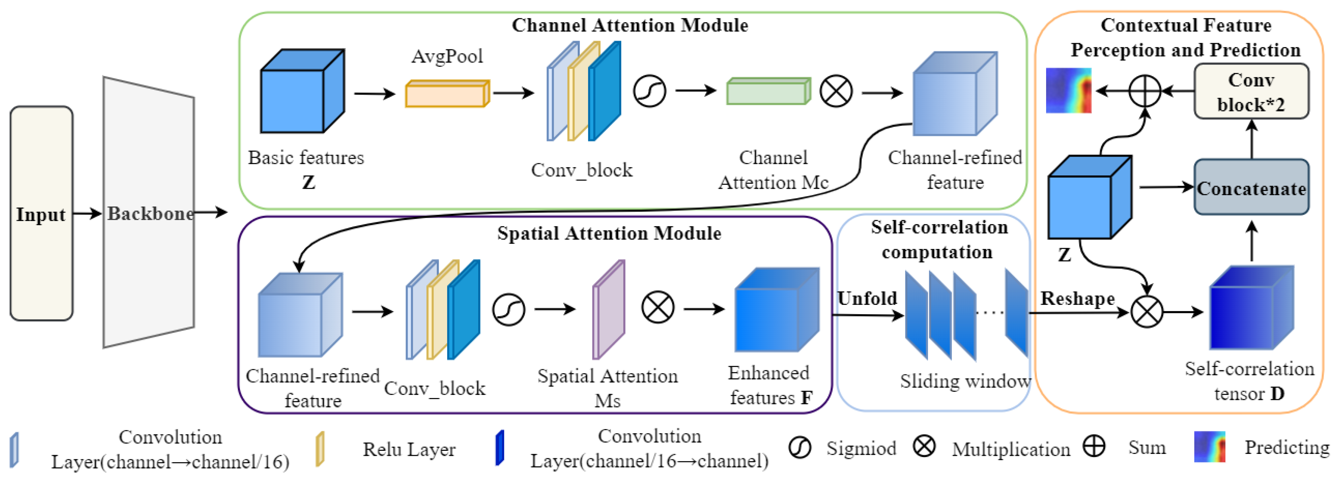
• This paper proposes a new autocorrelation semantic enhancement method (ASE), which enhances the base features and extracts important local area features through CS attention and autocorrelation modules.
• By combining the backbone network and the autocorrelation semantic enhancement module, our model ASENet can solve the problems of information loss, feature ambiguity, and confusion that traditional neural network models would have when dealing with low-resolution steel defect images.
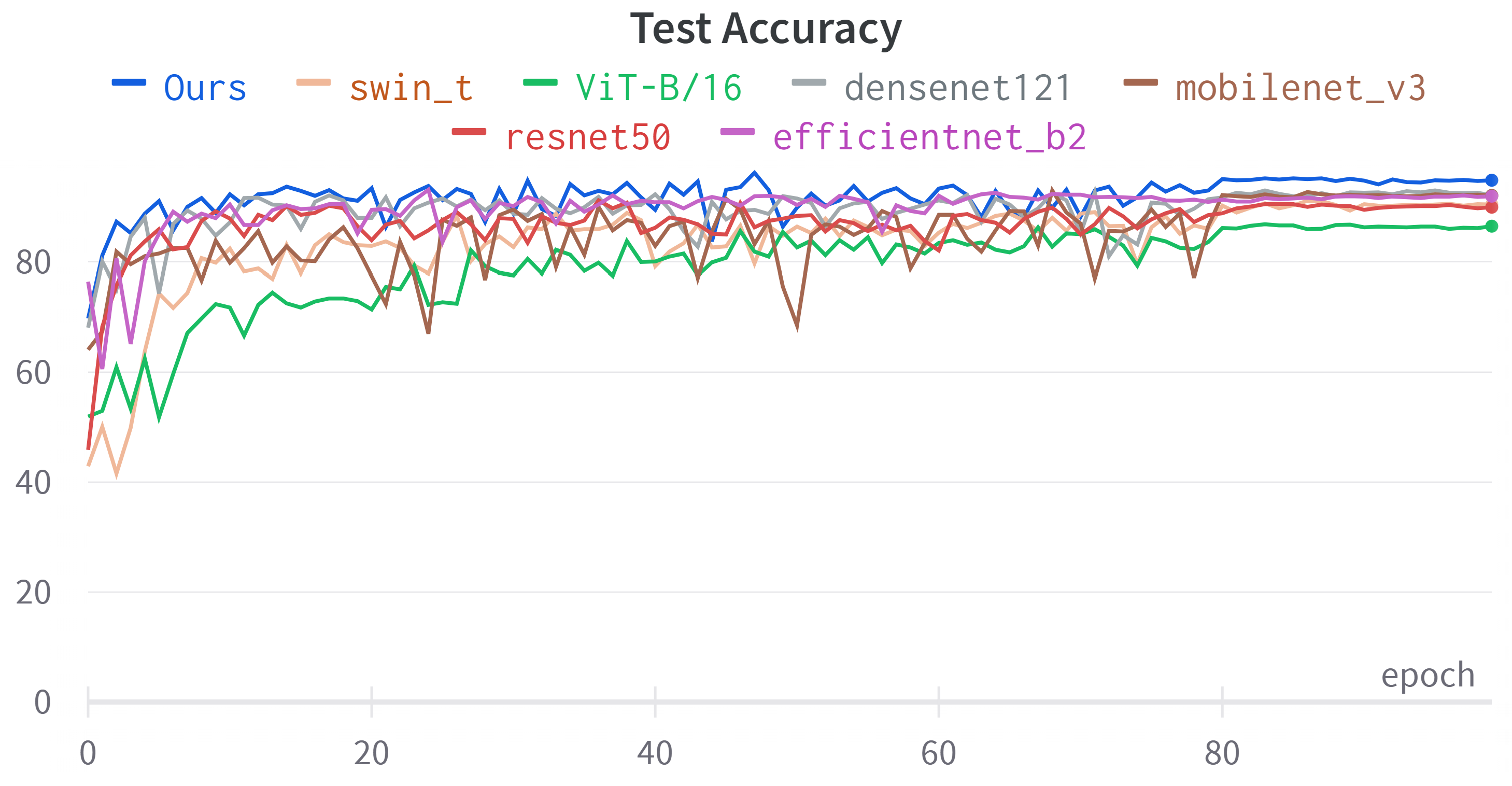
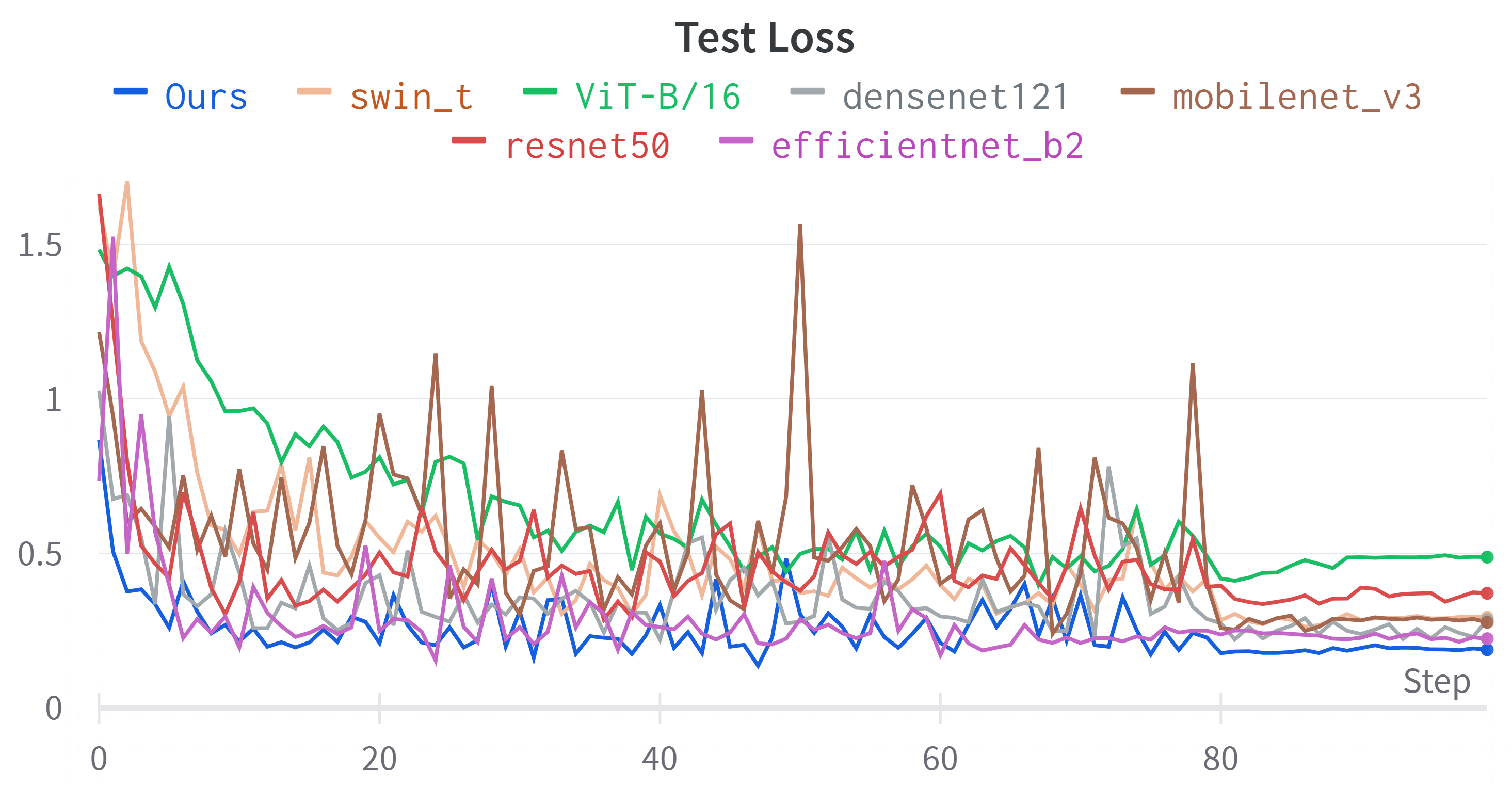
• Significant classification accuracies are achieved on the NEU-CLS-64 and CIFAR-100 datasets, and comparisons with several benchmark models demonstrate the effectiveness and superiority of the method.

2. Related Work

2.1. Classification of Steel Defects

Conventional methods for identifying defects on steel surfaces mainly use the wavelet transform [13,14] double-threshold binarization [15,16], and decision trees [17,18] to analyze and detect images. In addition to this, Mukhopadhyay et al. used multi-scale morphological segmentation of gray-scale images to process surface image data [19]; Podulka et al. used surface topographic image (STI) processing to characterize selected features from the surface texture [20]; and Ravimal et al. used the intensity of the near-field contrast image after reflecting light and reflective mirrors, as well as photometric stereoscopic techniques to recover the normal of the surface mapping for automated surface inspection [21]. By adopting these techniques, great strides have been made in optimizing productivity and improving product quality. However, these traditional methods have limitations. An obvious disadvantage is the relatively slow detection speed and the limited applicability. The algorithms used in these technologies often require substantial redesign for different application scenarios. This requirement not only increases the complexity of the process but also poses a significant obstacle to its widespread application. Another limiting factor is the high image quality requirement. When the input image is of low resolution, due to the small number of pixels in the low-resolution image, many details and information cannot be expressed in the picture, resulting in a decrease in detection accuracy.

Some recent approaches use convolutional neural networks for steel defect detection. These techniques are particularly effective in natural scenes, where they have gained substantial research support. For instance, Li et al. utilized coordinate attention and self-interaction to identify hot-rolled strip surface defects [22] effectively. Furthermore, Hao et al. proposed a novel two-stream neural network with sample generation and transfer learning for classifying steel strip surface defects [23]. Zhang et al. contributed to this growing research by proposing a novel approach for accurately classifying strip surface defects using generative adversarial networks and attention mechanisms [24]. Li et al. took a different approach by submitting a hybrid network architecture (CNN-T) that merged the CNN and Transformer encoders, achieving significant results on the NEU-CLS dataset [25]. However, these methods also require high-quality defect images.

Therefore, we proposed the ASENet network for low-resolution steel surface defect images to solve the problems of blurred edges and contours of low-resolution defect images, which lead to information loss, blurred features, and easy confusion.

2.2. Attention Mechanism

The purpose of the attention mechanism is to let the system learn to focus on areas of interest or high value from a large amount of information. It has now been successfully applied to various tasks [26,27,28,29]. For example, the self-attention mechanism used in the Transform model in 2017 has become a significant turning point in developing large-scale models [10]. Furthermore, SENet [30] introduces a channel attention block for image classification; it assigns attention weights to different input channels, allowing the network to focus on the most informative channels. Building upon this, the ECANet [31] further improved upon the SENet’s strategy by proposing an adequate channel attention (ECA) block for convolutional neural networks (CNNs), successfully enabling cross-channel interaction. CBAM introduces the channel and spatial attention modules to establish the dual mechanism of channel and spatial attention [32]. While computing image autocorrelation, conventional approaches often rely on neighborhood correlation [33,34]. However, this approach is computationally intensive and adds complexity to the model.

In contrast, the ASE module proposed in this paper achieves contextual feature awareness through simple connections after enhancing basic features, eliminating the need for many redundant parameters. This module allows the model to capture dependencies between adjacent elements in the input, enhancing contextual understanding.

3. Our Approach

In this section, we focus on the specific implementation of ASENet. Figure 1 shows the overall architecture of the network. ASENet mainly consists of a backbone network and ASE modules. The ASE modules consist of three main learnable modules: the CS attention module, the autocorrelation computation module, and the contextual feature-aware module, as shown in Figure 2.

3.1. Overall Architecture

Given a set of steel defect sample images, we extract basic features $Z\in {\mathbb{R}}^{H\times W\times C}$ using a backbone network. Subsequently, we augment these basic features by the CS attention module to obtain the augmented feature representation $F\in {\mathbb{R}}^{H\times W\times C}$. The autocorrelation is then computed on the augmented feature F to obtain the autocorrelation tensor $Din{\mathbb{R}}^{H\times W\times C_1}$ ($C_1=U\times V\times C$) and contextualized with the base feature Z to produce the self-attention feature $A\in {\mathbb{R}}^{H\times W\times C_g}$ ($C_g=C^{\prime }+C$). Finally, the resulting features are passed through two output convolutional layers to recover the number of channels and residual to derive the final output $G\in {\mathbb{R}}^{H\times W\times C}$ from the basic features.

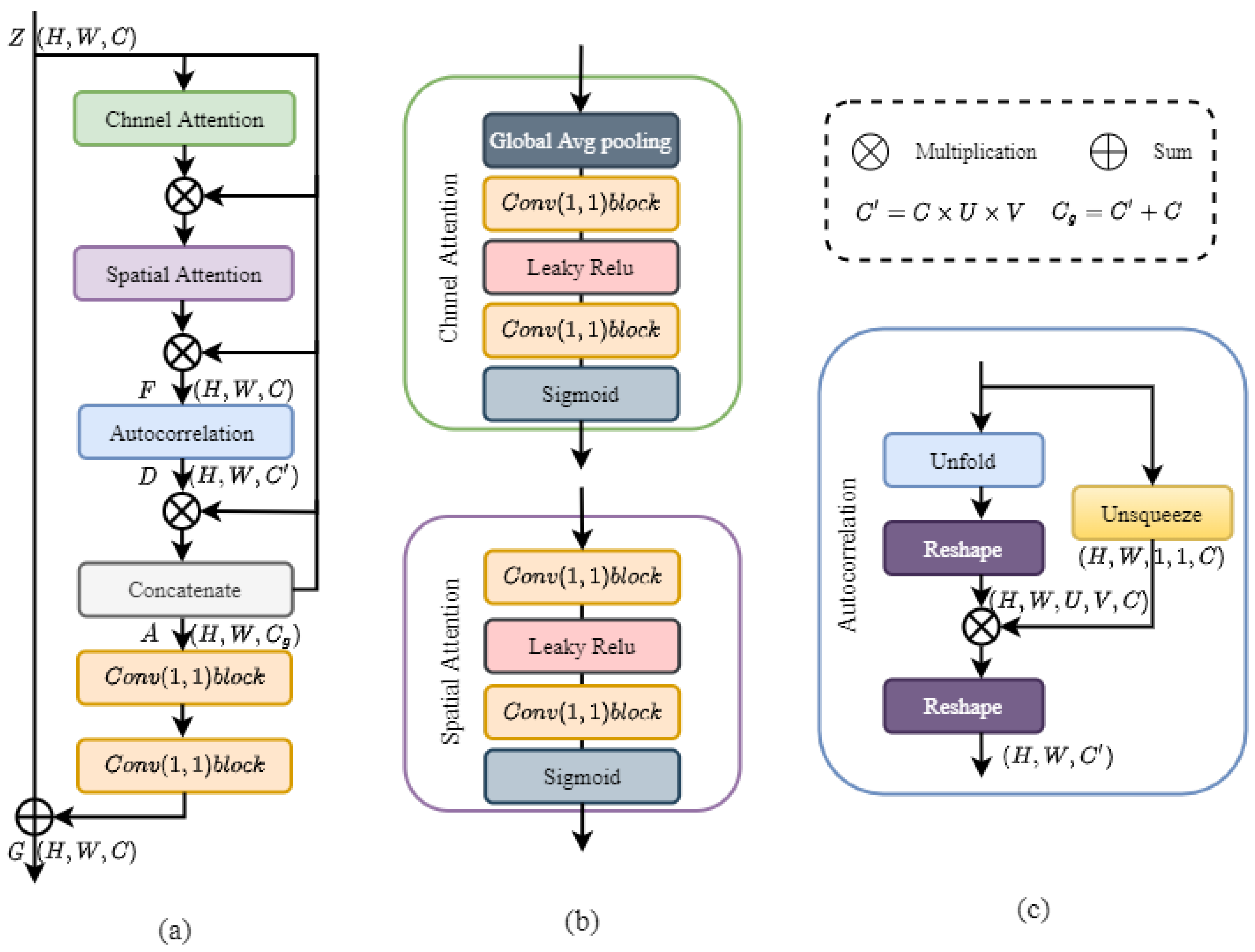
3.2. CS Attention Module

We devised a CS attention method to enhance the channel and spatial information in the basic features. This method consists of two complete modules: the channel and spatial attention modules, as shown in Figure 2b. These modules collaborate to generate the attention weights, which are essential for determining the importance of each track and its spatial location in the feature.

We calculate each channel’s attention weight within the channel attention module, denoted as $M_c$. Specifically, we begin by processing the foundational features using average pooling, followed by their refinement through a convolutional block. We subsequently map the final result to an output range between 0 and 1, achieved via a Sigmoid function, thereby obtaining the channel attention weight $M_c$. This weight effectively mirrors the importance of each channel in capturing pertinent information. We can prioritize the channels with information-rich content by assigning higher weights to channels housing valuable insights and lower weights to those contributing less.

Similarly, within the spatial attention module, we generate attention weights, denoted as $M_s$, for each spatial location within the feature. In this case, we employ a convolutional block to directly learn the features and subsequently map the results to an output range constrained between 0 and 1, once again utilizing a Sigmoid function. This process yields the spatial attention weight $M_s$, which signifies the significance of each pixel location in capturing meaningful insights. We can effectively concentrate on the pivotal spatial positions that drive understanding and context by attributing higher weights to areas that substantially contribute to the overall comprehension of the data and lower consequences to those of lesser informative value. Through the weights obtained by $M_c$ and $M_s$, we can get the final enhanced feature $F\in {\mathbb{R}}^{H\times W\times C}$.

$$F=Z\times M_c\times M_s$$

(1)

Unlike previous approaches [32], we have not utilized global max pooling to capture weights in channel and spatial dimensions or employed MLP (multi-layer perceptron) for feature extraction. Instead, we have used a convolutional approach to extract feature information. Additionally, in our CS attention module, we employed a single branch to learn the relationship between channel and spatial positions. Our experiments have revealed that lightweight attention modules are more suitable for low-resolution and blurry image processing tasks while avoiding unnecessary computations.

3.3. Autocorrelation Computation Calculation

To capture the self-similarity of neighborhoods in the image, we employ a calculation method that involves the Hadamard product. This product is performed between the C-dimensional vectors at each position x in the enhanced feature $F\in {\mathbb{R}}^{H\times W\times C}$ and their corresponding values in the neighborhood. The resulting products are then collected into a self-correlation tensor denoted as $\mathbf{D}\in {\mathbb{R}}^{H\times W\times C_1}$. The self-correlation tensor D. represents the relationships between different positions in the image. It allows us to identify patterns and similarities within local neighborhoods. We can obtain a tensor that expresses these relationships by calculating the Hadamard product and accumulating the results into D. The dimensionality of D is represented by $C_1$, corresponding to the channel of output vectors.

$$D(x,p)=\frac{Z\left(x\right)}{\parallel Z\left(x\right)\parallel }\odot \frac{F(x+p)}{\parallel F(x+p)\parallel }$$

(2)

where $p\in \left[-d_U,d_U\right]\times \left[-d_V,d_V\right]$ corresponds to the relative positions in the neighborhood window. Here, $d_U$ and $d_V$ represent the maximum displacement in the horizontal and vertical directions, respectively. The window size is determined by $U=2d_U+1$ and $V=2d_V+1$, which includes the center position. Our experiments use a sliding window of $(U,V)\in (1,1)$. Unlike previous work [35], we do not keep the dimension of $U\times V$, but consider it as part of the channel features so that we can obtain the new channel dimension $C_1=U\times V\times C^{\prime }$.

3.4. Contextual Feature Perception

Even though autocorrelation computing may determine how similar two images are to one another, it lacks the local semantic cues that the original convolutional features provided. We use a straightforward fusion step to create a contextual feature-aware semantic representation to capture various properties of the semantic objects. We specifically sew Z and D together to make the contextual semantic characteristics $\mathrm{A}\in {\mathbb{R}}^{H\times W\times C_g}$, as shown below.

$$A_{(i,j)}={\left[Z_{(i,j)}^{\mathrm{T}},D_{(i,j)}^{\mathrm{T}}\right]}^{\mathrm{T}}$$

(3)

To analyze the contextual relationships in A, convolution and bulk normalization operations are performed through the first convolutional layer to extract more semantically meaningful feature information. The extracted feature tensor is then subjected to a re-convolution operation to reduce the number of feature channels to the number of input channels to obtain a more compact feature representation. The convolution kernels for the two above convolutions’ blocks are both of size $1\times 1$. The convolution block $h\left(\right)$ learns contextual relationships without padding and aggregates local correlation patterns, restoring the channel dimension to C, ensuring that the output $h\left(h\right(A\left)\right)$ is the same size as Z. We then combine these two representations to generate the final feature representation $G\in {\mathbb{R}}^{H\times W\times C}$.

$$G=h\left(h\right(A\left)\right)+Z$$

(4)

Using an autocorrelation semantic enhancement network to augment the basic features helps to locate the essential regions of the target object. It enhances the recognizability of the features, which better achieves accurate classification in low-resolution images and improves the network’s performance.

4. Experimental Results

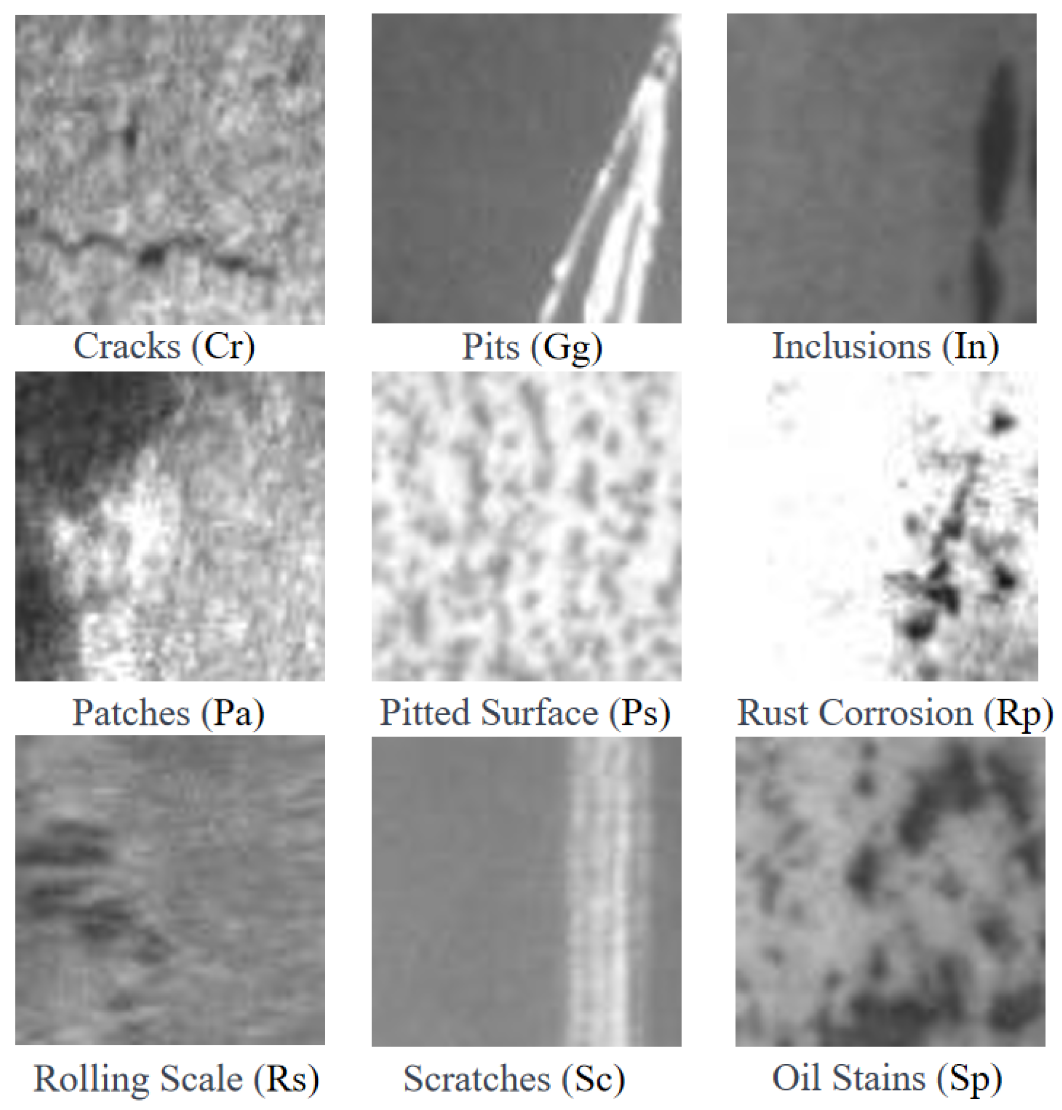
In this section, we evaluate the performance of ASENet on the NEU-CLS-64 and CIFAR-100 datasets and compare it to other methods. In addition, we perform ablation studies and compare them with other attention methods to validate the effectiveness of the autocorrelation semantic enhancement networks. Figure 3 shows the test results of different models running 100 epochs on the NEU-CLS-64 dataset under the same experimental setup. Figure 4 shows the loss curves for the other models.

4.1. Dataset

In the Northeastern University (NEU) Surface Defect Database [12], six typical surface defects of hot-rolled steel strips are collected, namely rolling scale (RS), patches (Pa), cracks (Cr), pitting surface (PS), inclusions (In), and scratches (Sc). The NEU-CLS-64 dataset used in this experiment includes an additional three defects: oil stains (Sp), pits (Gg), and rust (Rp). Furthermore, compared to the NEU dataset, all images in the NEU-CLS-64 dataset are of a fixed size of 64 × 64 pixels. The number of images per category varies (for instance, the pits (Gg) category has 296 images, while the oil stains (Sp) category has 438 images), as shown in Figure 5. CIFAR-100 is a widely used dataset in computer vision research. It consists of 60,000 color images, each of size 32 × 32 pixels, belonging to 100 different classes. The dataset is divided into two sets: a training set with 50,000 images and a test set with 10,000 images. This lower-resolution imagery undoubtedly poses more significant challenges for accurate classification by the neural network.

4.2. Experimental Details

This study conducted experiments using the PyTorch 1.8 deep learning framework on a system equipped with an NVIDIA 2080Ti GPU and an Intel i7 9700K CPU. The NEU-CLS-64 dataset is divided into training and test sets in the ratio of 80:20, where 80% of the data is used for training, and the remaining 20% is used for testing, and CIFAR-100 uses 500 images of each class as the training set and 100 images as the test set. In these experiments, the NEU-CLS-64 input image size is 64 × 64 pixels, CIFAR-100 input image size is 32 × 32 pixels, ConvNet-4 is used for the backbone network, and 3 × 3 convolution kernels are used for each convolutional block. The number of channels in each Conv block increased to 64-160-320-640 to capture more semantic information in the feature maps. For optimization, the SGD (stochastic gradient descent) optimizer was used with a momentum of 0.9. The initial learning rate was set at 0.01, with a decay factor of 0.05. The training was performed on the NEU-CLS-64 dataset for 100 epochs, with a batch size of 64 samples. Learning rate annealing was applied after the 80th and 90th epochs by reducing the learning rate by 0.1.

4.3. Results

Table 1. Comparison results with other methods on the NEU-CLS-64 and CIFAR-100 dataset.

Method	NEU-CLS-64	CIFAR-100	Params Size (M)	FLOPs (G)
ViT-B/16 [36]	86.81	56.19	326.74 MB	93.09 GFLOPs
Swin_t [37]	91.09	58.24	71.94 MB	47.33 GFLOPs
ResNet50 [38]	91.37	61.08	89.75 MB	21.59 GFLOPs
Mobilenet_v3_small [39]	92.90	59.44	5.83 MB	0.38 GFLOPs
Densenet121 [40]	92.96	66.30	31.01 MB	15.13 GFLOPs
Efficientnet_b2 [41]	93.23	60.32	34.75 MB	3.74 GFLOPs
ASENet (Ours)	96.24	71.66	3.04 MB	17.61 GFLOPs

shows that on the NEU-CLS-64 dataset, the proposed method outperforms all other methods in terms of accuracy, achieving an impressive 96.24%. Compared to ViT-B/16, Swin-t, ResNet50, MobileNetV3 Small, DenseNet121, and EfficientNetB2, it achieves an improvement of 9.43%, 5.15%, 4.87%, 3.34%, 3.28%, and 3.01%, respectively. Figure 3 clearly illustrates that ASENet consistently maintains a high correct rate throughout the testing process. In contrast, ViT-B/16 exhibits a relatively smoother but substantially lower correct rate compared to the other models. Turning our attention to the loss curve, it becomes evident that ASENet achieves the lowest loss among the seven different model types and exhibits the smoothest loss curve, as depicted in Figure 4. Our method also achieved the best results on the CIFAR-100 dataset, showing that ASENet performs better even on a 32 × 32 pixel dataset. When considering the parameter size, our method stands out with only 3.04 MB, which is significantly smaller compared to other approaches. This implies that our method is more efficient in terms of memory usage.

It is worth noting that the latest ViT and Swin models exhibited the worst performance during the experiments. These two models have the most complex computations and parameters and deliver the poorest results. This can be attributed to the fact that when the input image size is small, the divided sub-patches are relatively tiny, containing limited information in each sub-patch. This limitation hinders the classifier from capturing sufficient information, thus affecting the model’s performance. Additionally, Transformer encoders have difficulty handling local features effectively. Therefore, traditional convolutional neural network (CNN) models perform better when dealing with low-resolution images.

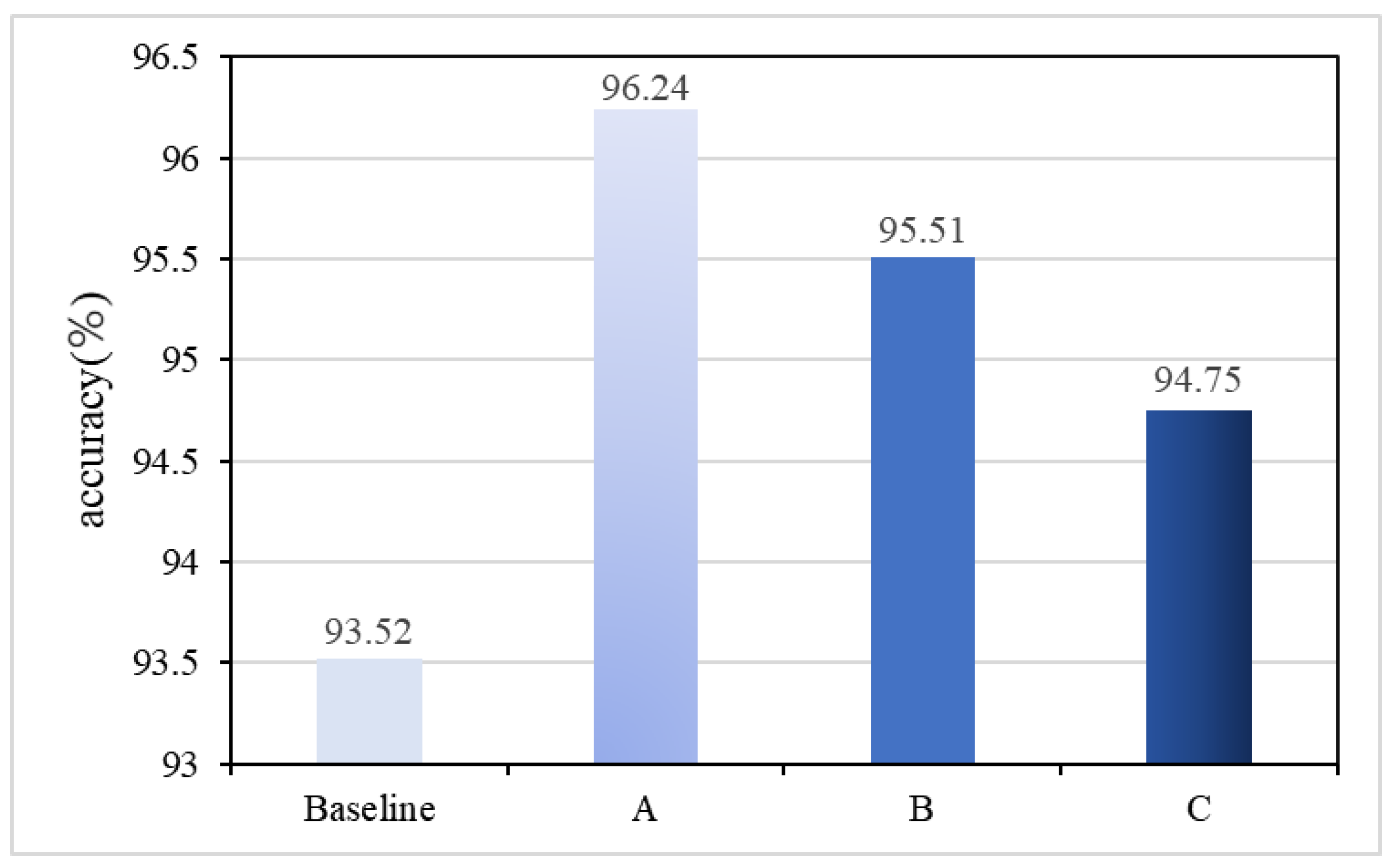
4.4. Ablation Studies

To evaluate the effectiveness of ASENet, we created a baseline model (ConvNet-4) without any additional modules. We performed ablation experiments on the NEU-CLS-64 dataset. As shown in

Table 2. Adding the effects of different modules.

Id	CS Attention	Autocorrelation Computation	Contextual Feature	Accuracy (%)
(a)	×	×	×	93.52
(b)	×	✓	✓	95.30
(c)	✓	×	✓	95.47
(d)	✓	✓	×	95.68
(e)	✓	✓	✓	96.24

, we compare the three learnable modules in two-by-two combinations with the baseline model and ASENet. In scenario (b), where only autocorrelation computation and contextual features are used, the accuracy achieved is 95.30%. Adding the CS attention module in method (c) slightly increases the accuracy to 95.47%. Similarly, including autocorrelation computation in scenario (d) with the CS attention module but without contextual features results in an accuracy of 95.68%. However, the most impressive improvement in accuracy is observed in scenario (e), where all three modules are used concurrently. An accuracy of 96.24% is achieved, the highest among all the methods.

Moreover, to analyze the impact of different values of the sliding window $(U,V)$ on the network’s autocorrelation computation, we conducted a comparison between $(U,V)\in (1,1)$, $(U,V)\in (3,3)$, and $(U,V)\in (5,5)$, which we named as A, B, and C, respectively. It is important to note that $(U,V)\in (1,1)$, referred to as A, represents the sliding window used by ASENet. From Figure 6, it can be seen that as the value of $(U,V)$ increases gradually, the network performance decreases, which is due to the small size of the defective image, though the backbone-network-extracted feature maps are also relatively small, so a larger sliding window will lead to the loss of important information in the extraction process.

4.5. Comparison with Other Attention Modules

Table 3. Comparison results with other attention modules.

Method	Accuracy (%)	Params Size (M)	FLOPs (G)
Baseline	93.52	0 MB	0 GFLOPs
TripletAttention [42]	95.03	0.06 MB	0.14 GFLOPs
ShuffleAttention [43]	95.37	0.05 MB	0.01 GFLOPs
PSA [44]	95.44	0.78 MB	10.10 GFLOPs
CoTAttention [45]	95.45	1.08 MB	18.56 GFLOPs
MobileViTv2Attention [46]	95.51	1.17 MB	20.14 GFLOPs
Coord_attention [47]	95.65	0.07 MB	0.13 GFLOPs
SE [30]	95.68	0.08 MB	1.39 GFLOPs
CBAM [32]	95.76	0.10 MB	0.02 GFLOPs
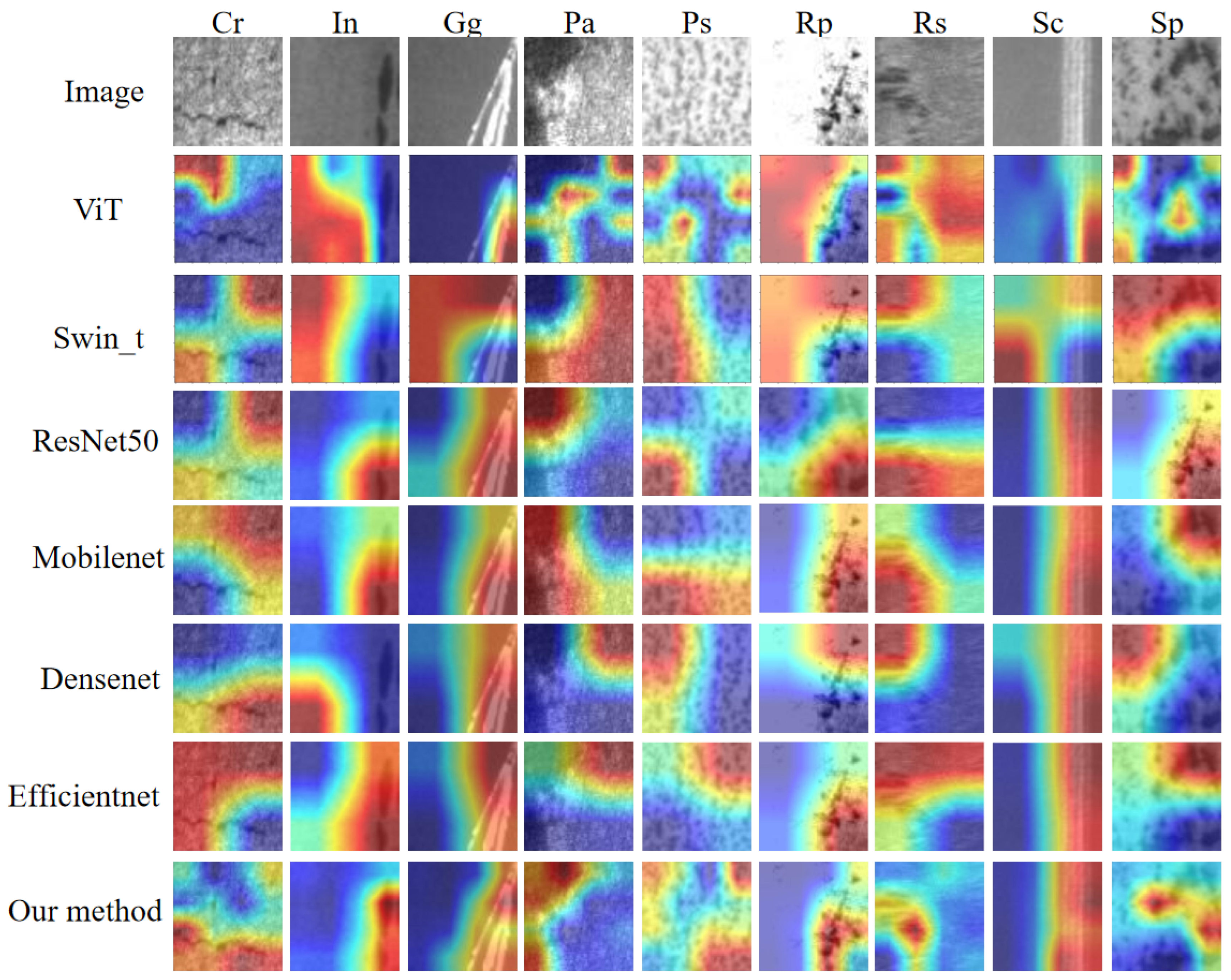
ASE (Ours)	96.24	1.27 MB	1.32 GFLOPs

compares the accuracy, number of parameters, and computational complexity of the autocorrelation semantic enhancement modules (ASE) and other attention modules. According to the study results, ASE outperforms other attention modules on NEU-CLS-64 by 2.72% over the baseline model. Although ASE performs well in accuracy, it is not the lightest in model parameter size. Regarding parameter size, ShuffleAttention is optimal at only 0.05 MB, while ASE has 1.27 MB of parameters. However, a slight parameter increase compared to performance may be acceptable, especially if computational resources allow it. Regarding computational complexity, our method is comparable mainly to the SE module, achieving the highest accuracy while maintaining competitive parameter sizes and computational complexity. This demonstrates the effectiveness of our approach in capturing important features and improving classification accuracy.

4.6. Visualisation

Figure 7 showcases heatmap visualizations of various models [48]. The illustration reveals that the attention patterns in both the ViT and Swin models exhibit a more dispersed distribution. Conversely, the approach advocated in this paper, enhanced by the autocorrelation semantic enhancement module, effectively sieves out extraneous regions, channeling attention towards more pivotal image characteristics. Particularly for defects such as Cr, In, Pa, Rp, and Rs, it adeptly pinpoints their locations with superior accuracy compared to alternative methods. Furthermore, ASENet amalgamates features across diverse scales, rendering it more adept at discerning valuable features in intricate settings.

5. Conclusions

In this study, we propose the autocorrelation semantic enhancement network (ASENet) to address the challenge of imaging defects on low-resolution steel surfaces. ASENet consists of a backbone network and an ASE module, where the ASE contains a CS attention module, an autocorrelation computation module, and a contextual feature-aware module. The ASE module captures different aspects of feature semantics and enhances feature recognizability by augmenting the underlying features and computing correlations between neighboring domains. Experimental results on NEU-CLS-64 datasets show that the proposed ASENet can effectively solve the problems of defect type confusion, feature ambiguity, and low classification accuracy in low-resolution steel surface defect imaging. Compared with the existing models, the enhanced feature recognition capability of ASENet gives it superior performance, making it a promising method for steel surface defect classification.

References

1. Gardner, L. The use of stainless steel in structures. Prog. Struct. Eng. Mater. 2010, 7, 45–55. [Google Scholar] [CrossRef]
2. Wen, X.; Shan, J.; He, Y.; Song, K. Steel surface defect recognition: A survey. Coatings 2022, 13, 17. [Google Scholar] [CrossRef]
3. Chu, M.; Zhao, J.; Liu, X.; Gong, R. Multi-class classification for steel surface defects based on machine learning with quantile hyper-spheres. Chemom. Intell. Lab. Syst. 2017, 168, 15–27. [Google Scholar] [CrossRef]
4. Park, J.K.; Kwon, B.K.; Park, J.H.; Kang, D.J. Machine learning-based imaging system for surface defect inspection. Int. J. Precis. Eng.-Manuf.-Green Technol. 2016, 3, 303–310. [Google Scholar] [CrossRef]
5. Tang, B.; Chen, L.; Sun, W.; Lin, Z.k. Review of surface defect detection of steel products based on machine vision. IET Image Process. 2023, 17, 303–322. [Google Scholar] [CrossRef]
6. Wang, C.Y.; Bochkovskiy, A.; Liao, H.Y.M. YOLOv7: Trainable bag-of-freebies sets new state-of-the-art for real-time object detectors. In Proceedings of the IEEE/CVF Conference on Computer Vision and Pattern Recognition, Vancouver, BC, Canada, 8–22 June 2023; pp. 7464–7475. [Google Scholar] [CrossRef]
7. Cai, Z.; Vasconcelos, N. Cascade r-cnn: Delving into high quality object detection. In Proceedings of the IEEE Conference on Computer Vision and Pattern Recognition, Salt Lake City, UT, USA, 18–23 June 2018; pp. 6154–6162. [Google Scholar] [CrossRef]
8. Tian, Z.; Shen, C.; Chen, H.; He, T. Fcos: Fully convolutional one-stage object detection. In Proceedings of the IEEE/CVF International Conference on Computer Vision, Seoul, Republic of Korea, 27 October–2 November 2019; pp. 9627–9636. [Google Scholar]
9. Tan, M.; Pang, R.; Le, Q.V. Efficientdet: Scalable and efficient object detection. In Proceedings of the IEEE/CVF Conference on Computer Vision and Pattern Recognition, Seattle, WA, USA, 13–19 June 2020; pp. 10781–10790. [Google Scholar] [CrossRef]
10. Vaswani, A.; Shazeer, N.; Parmar, N.; Uszkoreit, J.; Jones, L.; Gomez, A.N.; Kaiser, Ł.; Polosukhin, I. Attention is all you need. Adv. Neural Inf. Process. Syst. 2017, 30. [Google Scholar]
11. Doersch, C. Tutorial on variational autoencoders. arXiv 2016, arXiv:1606.05908. [Google Scholar] [CrossRef]
12. Song, K.; Yan, Y. A noise robust method based on completed local binary patterns for hot-rolled steel strip surface defects. Appl. Surf. Sci. 2013, 285, 858–864. [Google Scholar] [CrossRef]
13. Zhang, S.; Karim, M. A new impulse detector for switching median filters. IEEE Signal Process. Lett. 2002, 9, 360–363. [Google Scholar] [CrossRef]
14. Wu, X.y.; Xu, K.; Xu, J.w. Application of Undecimated Wavelet Transform to Surface Defect Detection of Hot Rolled Steel Plates. In Proceedings of the 2008 Congress on Image and Signal Processing, Sanya, China, 27–30 May 2008; Volume 4, pp. 528–532. [Google Scholar] [CrossRef]
15. Senthikumar, M.; Palanisamy, V.; Jaya, J. Metal surface defect detection using iterative thresholding technique. In Proceedings of the Second International Conference on Current Trends In Engineering and Technology—ICCTET 2014, Coimbatore, India, 8 July 2014; pp. 561–564. [Google Scholar] [CrossRef]
16. Yun, J.P.; Kim, D.; Kim, K.; Lee, S.J.; Park, C.H.; Kim, S.W. Vision-based surface defect inspection for thick steel plates. Opt. Eng. 2017, 56, 053108. [Google Scholar] [CrossRef]
17. Aghdam, S.R.; Amid, E.; Imani, M.F. A fast method of steel surface defect detection using decision trees applied to LBP based features. In Proceedings of the 2012 7th IEEE Conference on Industrial Electronics and Applications (ICIEA), Singapore, 18–20 July 2012; pp. 1447–1452. [Google Scholar] [CrossRef]
18. Jian, L.; Wei, H.; Bin, H. Research on inspection and classification of leather surface defects based on neural network and decision tree. In Proceedings of the 2010 International Conference On Computer Design and Applications, Qinhuangdao, China, 25–27 June 2010; Volume 2, pp. V2-381–V2-384. [Google Scholar] [CrossRef]
19. Mukhopadhyay, S.; Chanda, B. Multiscale morphological segmentation of gray-scale images. IEEE Trans. Image Process. 2003, 12, 533–549. [Google Scholar] [CrossRef] [PubMed]
20. Podulka, P. Application of image processing methods for the characterization of selected features and wear analysis in surface topography measurements. Procedia Manuf. 2021, 53, 136–147. [Google Scholar] [CrossRef]
21. Ravimal, D.; Kim, H.; Koh, D.; Hong, J.H.; Lee, S.K. Image-based inspection technique of a machined metal surface for an unmanned lapping process. Int. J. Precis. Eng. Manuf. Green Technol. 2020, 7, 547–557. [Google Scholar] [CrossRef]
22. Li, Z.; Wu, C.; Han, Q.; Hou, M.; Chen, G.; Weng, T. CASI-Net: A novel and effect steel surface defect classification method based on coordinate attention and self-interaction mechanism. Mathematics 2022, 10, 963. [Google Scholar] [CrossRef]
23. Hao, Z.; Li, Z.; Ren, F.; Lv, S.; Ni, H. Strip steel surface defects classification based on generative adversarial network and attention mechanism. Metals 2022, 12, 311. [Google Scholar] [CrossRef]
24. Zhang, J.; Li, S.; Yan, Y.; Ni, Z.; Ni, H. Surface Defect Classification of Steel Strip with Few Samples Based on Dual-Stream Neural Network. Steel Res. Int. 2022, 93, 2100554. [Google Scholar] [CrossRef]
25. Li, S.; Wu, C.; Xiong, N. Hybrid architecture based on CNN and transformer for strip steel surface defect classification. Electronics 2022, 11, 1200. [Google Scholar] [CrossRef]
26. Bello, I.; Zoph, B.; Vaswani, A.; Shlens, J.; Le, Q.V. Attention augmented convolutional networks. In Proceedings of the IEEE/CVF International Conference on Computer Vision, Seoul, Republic of Korea, 27 October–2 November 2019; pp. 3286–3295. [Google Scholar]
27. Hu, D. An introductory survey on attention mechanisms in NLP problems. In Proceedings of the Intelligent Systems and Applications: Proceedings of the 2019 Intelligent Systems Conference (IntelliSys), London, UK, 3–4 September 2020; Volume 2, pp. 432–448. [Google Scholar] [CrossRef]
28. Fukui, H.; Hirakawa, T.; Yamashita, T.; Fujiyoshi, H. Attention branch network: Learning of attention mechanism for visual explanation. In Proceedings of the IEEE/CVF Conference on Computer Vision and Pattern Recognition, Long Beach, CA, USA, 15–20 June 2019; pp. 10705–10714. [Google Scholar]
29. Guo, M.H.; Xu, T.X.; Liu, J.J.; Liu, Z.N.; Jiang, P.T.; Mu, T.J.; Zhang, S.H.; Martin, R.R.; Cheng, M.M.; Hu, S.M. Attention mechanisms in computer vision: A survey. Comput. Vis. Media 2022, 8, 331–368. [Google Scholar] [CrossRef]
30. Hu, J.; Shen, L.; Sun, G. Squeeze-and-excitation networks. In Proceedings of the IEEE Conference on Computer Vision and Pattern Recognition, Salt Lake City, UT, USA, 18–23 June 2018; pp. 7132–7141. [Google Scholar] [CrossRef]
31. Wang, Q.; Wu, B.; Zhu, P.; Li, P.; Zuo, W.; Hu, Q. ECA-Net: Efficient channel attention for deep convolutional neural networks. In Proceedings of the IEEE/CVF Conference on Computer Vision and Pattern Recognition, Seattle, WA, USA, 13–19 June 2020; pp. 11534–11542. [Google Scholar]
32. Woo, S.; Park, J.; Lee, J.Y.; Kweon, I.S. Cbam: Convolutional block attention module. In Proceedings of the European Conference on Computer Vision (ECCV), Munich, Germany, 8–14 September 2018; pp. 3–19. [Google Scholar] [CrossRef]
33. Rocco, I.; Cimpoi, M.; Arandjelović, R.; Torii, A.; Pajdla, T.; Sivic, J. Neighbourhood consensus networks. Adv. Neural Inf. Process. Syst. 2018, 31. [Google Scholar]
34. Hassani, A.; Walton, S.; Li, J.; Li, S.; Shi, H. Neighborhood attention transformer. In Proceedings of the IEEE/CVF Conference on Computer Vision and Pattern Recognition, Vancouver, BC, Canada, 18–22 June 2023; pp. 6185–6194. [Google Scholar] [CrossRef]
35. Kang, D.; Kwon, H.; Min, J.; Cho, M. Relational embedding for few-shot classification. In Proceedings of the IEEE/CVF International Conference on Computer Vision, Montreal, QC, Canada, 10–17 October 2021; pp. 8822–8833. [Google Scholar] [CrossRef]
36. Dosovitskiy, A.; Beyer, L.; Kolesnikov, A.; Weissenborn, D.; Zhai, X.; Unterthiner, T.; Dehghani, M.; Minderer, M.; Heigold, G.; Gelly, S.; et al. An image is worth 16x16 words: Transformers for image recognition at scale. arXiv 2020, arXiv:2010.11929. [Google Scholar] [CrossRef]
37. Liu, Z.; Lin, Y.; Cao, Y.; Hu, H.; Wei, Y.; Zhang, Z.; Lin, S.; Guo, B. Swin transformer: Hierarchical vision transformer using shifted windows. In Proceedings of the IEEE/CVF International Conference on Computer Vision, Montreal, BC, Canada, 11–17 October 2021; pp. 10012–10022. [Google Scholar] [CrossRef]
38. He, K.; Zhang, X.; Ren, S.; Sun, J. Deep residual learning for image recognition. In Proceedings of the IEEE Conference on Computer Vision and Pattern Recognition, Las Vegas, NV, USA, 27–30 June 2016; pp. 770–778. [Google Scholar]
39. Howard, A.; Sandler, M.; Chu, G.; Chen, L.C.; Chen, B.; Tan, M.; Wang, W.; Zhu, Y.; Pang, R.; Vasudevan, V.; et al. Searching for mobilenetv3. In Proceedings of the IEEE/CVF International Conference on Computer Vision, Seoul, Republic of Korea, 27 October–2 November 2019; pp. 1314–1324. [Google Scholar]
40. Huang, G.; Liu, Z.; Van Der Maaten, L.; Weinberger, K.Q. Densely connected convolutional networks. In Proceedings of the IEEE Conference on Computer Vision and Pattern Recognition, Honolulu, HI, USA, 21–26 July 2017; pp. 4700–4708. [Google Scholar] [CrossRef]
41. Tan, M.; Le, Q. Efficientnet: Rethinking model scaling for convolutional neural networks. In Proceedings of the International Conference on Machine Learning. PMLR, Long Beach, CA, USA, 9–15 June 2019; pp. 6105–6114. [Google Scholar]
42. Misra, D.; Nalamada, T.; Arasanipalai, A.U.; Hou, Q. Rotate to attend: Convolutional triplet attention module. In Proceedings of the IEEE/CVF Winter Conference on Applications of Computer Vision, Virtual Conference, 5–9 January 2021; pp. 3139–3148. [Google Scholar] [CrossRef]
43. Zhang, Q.L.; Yang, Y.B. SA-Net: Shuffle Attention for Deep Convolutional Neural Networks. In Proceedings of the ICASSP 2021—2021 IEEE International Conference on Acoustics, Speech and Signal Processing (ICASSP), Toronto, ON, Canada, 6–11 June 2021; pp. 2235–2239. [Google Scholar] [CrossRef]
44. Liu, H.; Liu, F.; Fan, X.; Huang, D. Polarized self-attention: Towards high-quality pixel-wise regression. arXiv 2021, arXiv:2107.00782. [Google Scholar] [CrossRef]
45. Dai, Z.; Liu, H.; Le, Q.V.; Tan, M. Coatnet: Marrying convolution and attention for all data sizes. Adv. Neural Inf. Process. Syst. 2021, 34, 3965–3977. [Google Scholar]
46. Mehta, S.; Rastegari, M. Separable self-attention for mobile vision transformers. arXiv 2022, arXiv:2206.02680. [Google Scholar] [CrossRef]
47. Hou, Q.; Zhou, D.; Feng, J. Coordinate attention for efficient mobile network design. In Proceedings of the IEEE/CVF Conference on Computer Vision and Pattern Recognition, Nashville, TN, USA, 20–25 June 2021; pp. 13713–13722. [Google Scholar] [CrossRef]
48. Selvaraju, R.R.; Cogswell, M.; Das, A.; Vedantam, R.; Parikh, D.; Batra, D. Grad-cam: Visual explanations from deep networks via gradient-based localization. In Proceedings of the IEEE International Conference on Computer Vision, Venice, Italy, 22–29 October 2017; pp. 618–626. [Google Scholar]
Figure 1. The overall architecture of ASENet.
Coatings 13 02015 g001
Figure 2. (a) ASE modules, (b) CS attention module, and (c) autocorrelation calculation.
Coatings 13 02015 g002
Figure 3. Test results of different models running 100 epochs on the NEU-CLS-64 dataset.
Coatings 13 02015 g003
Figure 4. Loss curves of different models running on the NEU-CLS-64 dataset for 100 epochs.
Coatings 13 02015 g004
Figure 5. Sample images of 9 typical surface defects in the NEU-CLS-64 dataset.
Coatings 13 02015 g005
Figure 6. The impact of U and V values on the network.
Coatings 13 02015 g006
Figure 7. Results of different model visualizations.
Coatings 13 02015 g007