Mathematical Model of Surface Topography of Corroded Steel Foundation in Submarine Soil Environment

Abstract

For the corrosion risk of steel structures in the marine environment, the topography characteristics of corroded steel surfaces were paid little attention to, which has a significant effect on the mechanical properties of the interface between steel foundation and soil medium. An effective mathematical model for reconstructing the topography of corroded steel surface is very helpful for numerically or experimentally studying the soil-corroded steel interaction properties. In this study, an electrolytic accelerated corrosion experiment is conducted first to obtain corroded steel samples, which are exposed to submarine soil and suffer different corrosion degrees. Then, the surface height data of these corroded steel samples are scanned and analyzed. It is found that the height of surface two-dimensional contour curves under different corrosion degrees obeys the Gaussian distribution. Based on the spectral representation method, a mathematical model is developed for the profile height of the corroded steel surface. By comparing the standard deviation, arithmetic mean height and maximum height of reconstructed samples with those of experimental samples, the reliability of the developed mathematical model is proved. The proposed mathematical model can be adapted to reconstruct the surface topography of steel with different corrosion degrees for the following research on the shearing behavior of soil-corroded steel interface.

1. Introduction

It is a common phenomenon during the service life of steel structures in the marine environment. With the rapid development of exploitations of marine energy, the salt corrosion research of steel structures has been focused on widely [1]. In design, the protective layer and surplus design are often considered to reduce the effect of corrosion [2,3]. However, as time goes on, the protection system may fail. Corrosion will happen and affect the property of the steel structure. Therefore, it is important to study the corrosion characteristics of steel structures in a marine environment.

At present, a large number of studies has been conducted on the corrosion characteristics of steel material in a corrosive environment, with the aid of experiment methods and modern analytical techniques. The relevant research can be found in the work of Kovendhan et al. [4], James and Hattingh [5], Lv et al. [6], Wei et al. [7] and so on. The above studies mainly focus on explaining the occurrence of metal corrosion in terms of lattice and electrochemical mechanisms. However, civil engineers care more about the mechanical properties and residual bearing capacity of steel members or structures after corrosion. There are different methods to consider the effect of corrosion on steel structures. Some researchers simulated the effect of corrosion on the mechanical behavior of steel structures by decreasing the section thickness of steel members. Karagah et al. [8] investigated the effect of corrosion on the axial capacity of short steel columns by reducing the localized thickness in a monotonic axial load experiment. Liu et al. [9] notched in the center zone of steel columns to simulate the loss of section due to corrosion in axial loading tests. Wang et al. [10,11] analyzed the ultimate strength of steel pipe piles in corrosion conditions by converting corrosion effects into thickness loss in numerical simulations. Other similar studies can be found in the literature by Yamamoto and Ikegami [12], Akpan et al. [13], Guo et al. [14] and so on. The above research studies only consider the effect of section thickness loss due to corrosion but ignore the effect of variation of the surface topography of steel structures. To consider the effect of surface topography, Jiang and Soares [15] assumed corrosion pits to be cylindrically shaped with various distributions and intensity or depth in numerical analysis. Ahmmad and Sumi [16] considered the corrosion pit as conical pits with different depth-to-diameter ratios. Nakai et al. [17,18] studied the effect of corrosion on steel plate strength by artificially creating conical corrosion pits in experiments and numerical simulations. Though some researchers have already begun to study the effect of corroded surface topography on the mechanical properties of steel members or structures, the corroded surface topography is always considered simply by setting pits with regular shape and distribution, which is difficult to describe the real surface topography of corroded steel structure. Little research has been devoted to the shearing property of soil-corroded steel surface, which has a significant influence on the bearing capacity of the steel foundation of ocean structures. The main reason can be attributed to the lack of an effective mathematical model of the surface topography of corroded steel.

In this paper, the corrosion characteristics of Q235 steel in a submarine clay soil environment are studied by electrolytic accelerated corrosion experiments. The electrochemical process of corrosion and the law of mass loss are analyzed. To further characterize the corroded steel surface, the surface topography is investigated. After the analysis of two-dimensional profile height on a corroded surface, a mathematical model is constructed by the spectral representation method. The reliability of the mathematical model is verified. The developed model can be employed to generate the surface profile of corroded steel structures as close as possible to the reality in the follow-up research. It is very helpful for studying the corrosion characteristic of the steel surface and the soil-corroded steel interaction properties.

2. Electrolytic Accelerated Corrosion Experiment

Electrolytic accelerated corrosion experiment is a common method for the investigation of the corrosion of metals [19,20,21]. The acceleration mechanism is to accelerate the electrochemical reaction of the corroded metal by means of an applied current [22]. Compared with natural exposure experiments, the electrolytic accelerated corrosion experiment is more convenient and can save a lot of time. In this study, the electrolytic accelerated corrosion experiment is conducted to investigate the corrosion characteristic of steel structure foundation in submarine soil.

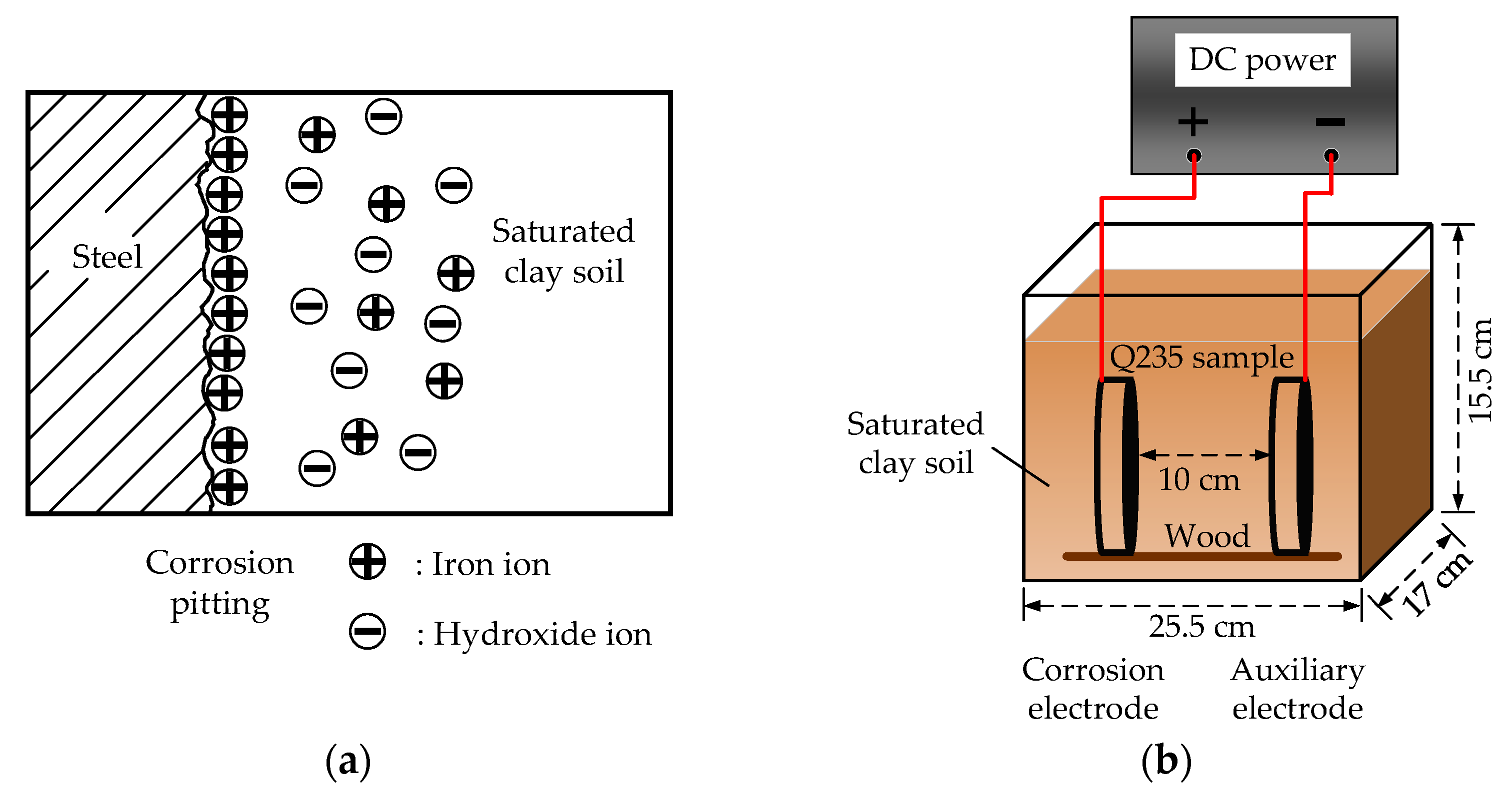
2.1. Experimental Principle

The electrolytic accelerated corrosion is a result of an artificial electrolytic cell reaction. Figure 1a shows the electrochemical reaction process on the surface of the corroded specimen. The corroded electrode loses electrons and undergoes an oxidation reaction, while the electrolyte solution gains electrons for a reduction reaction [19,21,23].

The anodic reaction can be represented as

$$Fe\to F{e}^{2+}+2e^{-}$$

(1)

$$Fe\to F{e}^{3+}+3e^{-}$$

(2)

The cathode reaction can be represented as

$$O_2+2H_{2}O+4e^{-}\to 4O{H}^{-}$$

(3)

The corrosion current is controlled by the applied current during experiments. According to Faraday law [19,21], the theoretical mass loss of electrochemical corrosion can be calculated as

$$\Delta m=\frac{MIT}{zF}$$

(4)

where M represents the molar mass of Fe (56 g·mol⁻¹); I is the experimental current (A); t is the experimental time (s); z is the number of electrons transferred by corrosion of Fe (z = 2 or 3); F is Faraday constant which has a value of 96,500 A·s⁻¹.

2.2. Experimental Process

The experiment is mainly composed of a direct current (DC) power, a glass container, clay soil, an electrolyte solution and a Q235 steel sample. The experiment system is shown in Figure 1b. The Q235 steel is machined to circular samples with a diameter of 61.5 mm and a thickness of 10 mm. In the experimental process, one sample is used as the corrosion electrode connected to the positive pole of DC power; the other is connected to the negative terminal of the power supply as an auxiliary electrode. Throughout the experiment, the two electrodes are fixed in position by a wooden rod and kept 10 cm apart. Waterproof tape is used to wrap the corrosion electrode, leaving only one side. By maintaining a constant current of 3 A throughout the experiment, the corrosion process of the steel sample connected to the positive pole is accelerated. Saturated clay soil is used to simulate the submarine soil environment, which is derived from the coastal region. A 5% mass concentration NaCl solution is added to the clay soil as an electrolyte solution.

After the experiment, the corroded steel sample is removed from the experimental apparatus and cleaned. The whole experiments are set up with ten groups of working conditions with a minimum experimental time of 1 h and a maximum experimental time of 10 h. The duration of each group of experiments differs by one hour. In addition, the uncorroded steel sample is used for a control group.

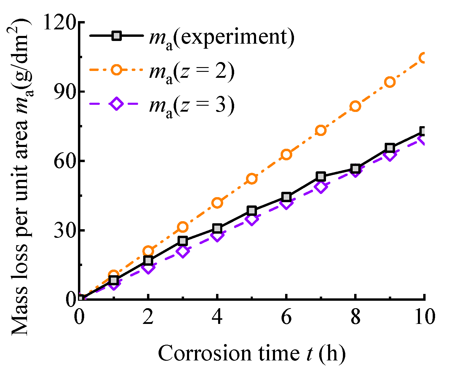
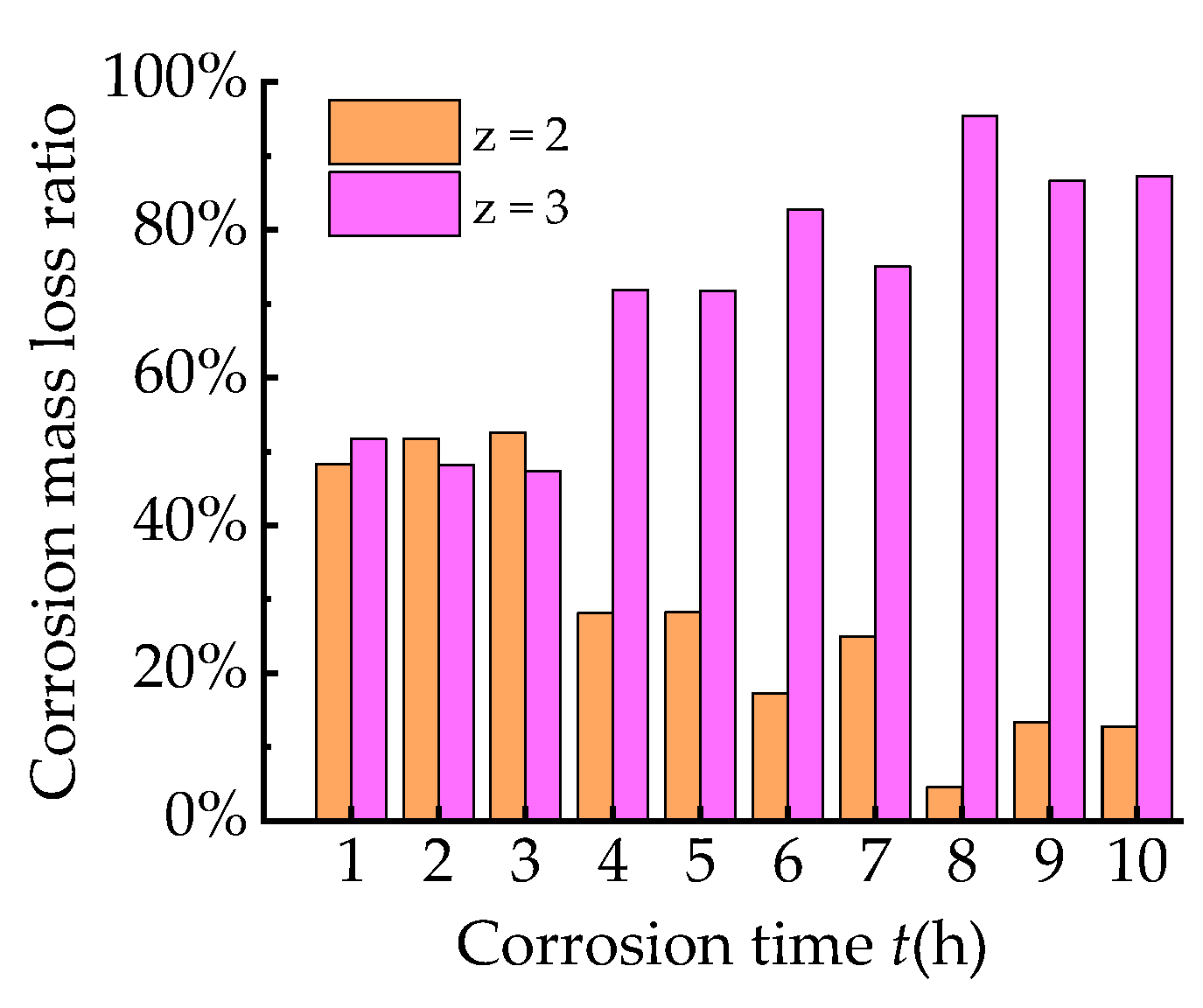
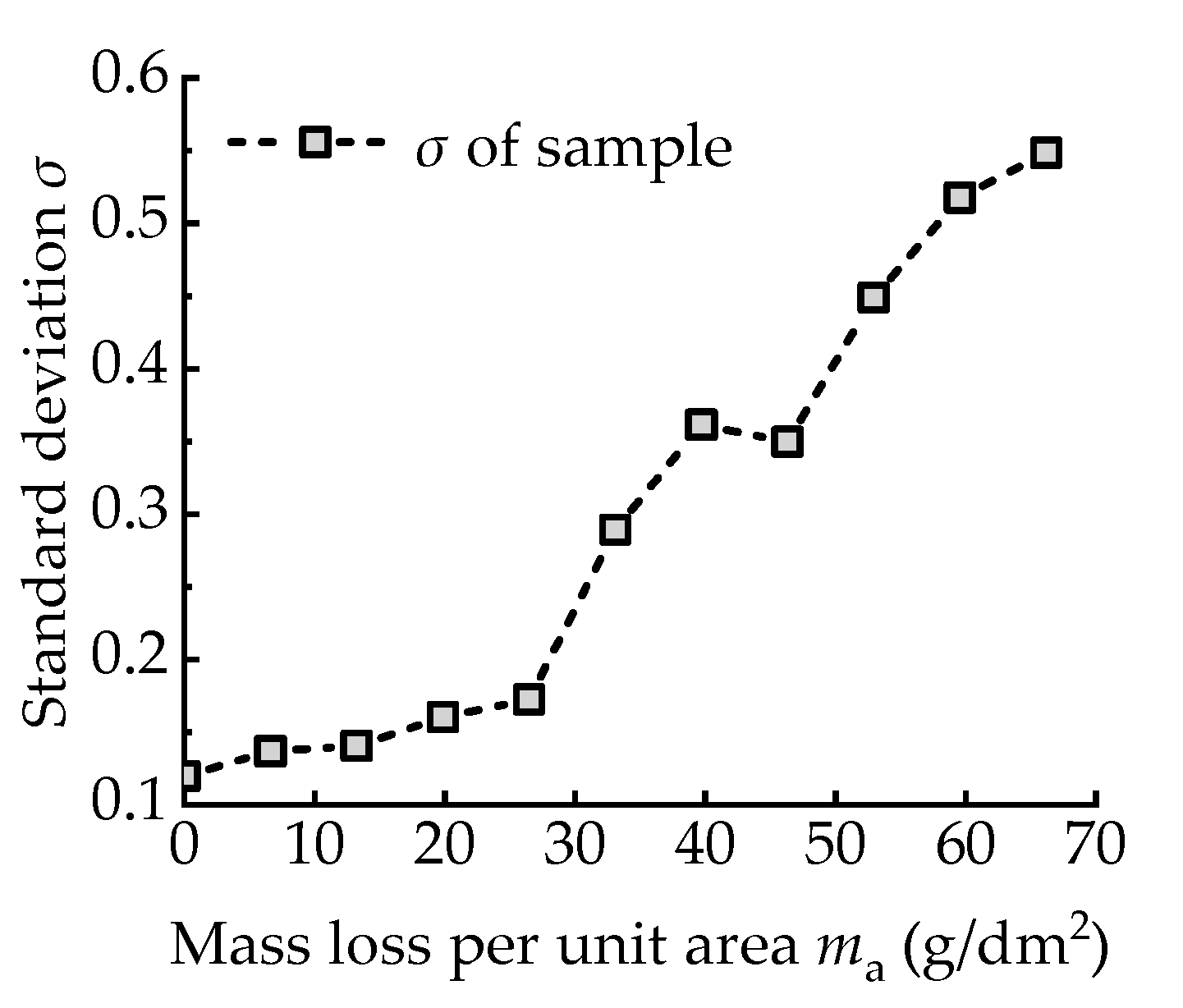
2.3. Mass Loss per Unit Area

After experiments, the corroded samples are removed from the soil and tore off the waterproof tapes. Then the corrosion products are cleaned. The fragile corrosion products stuck to the surface can be easily removed by flowing water. The rest of the corrosion products are cleaned with ethyl alcohol and distilled water. After drying, the samples are weighed. The mass loss per unit area m_a is employed to describe the corrosion degree of the samples, which is calculated as

$$m_a=\frac{m_0-m_1}{A}=\frac{m_0-m_1}{\pi r^2}$$

(5)

where m_a is the mass loss per unit area (g/dm²); m₀ is the original weight of the sample (g); m₁ is the weight of the corroded sample (g); A is the area of the corroded surface (dm²), which can be given by the radius r of the circular surface as πr².

Based on Equation (4), the theoretical values of mass loss per unit area under different corrosion times are calculated by taking z to be 2 and 3, respectively, wherein z represents the number of electrons transferred by corrosion of Fe. When z equals 2, the corrosion product is divalent iron, and when z equals 3, the corrosion product is trivalent iron. The comparison between the experimental value and the theoretical value is shown in Figure 2. One finds from Figure 2 that the mass loss per unit area measured by experimental samples is between the theoretical values calculated with z being 2 and 3. It means the experimental corrosion products included both trivalent iron and divalent iron. Another phenomenon can be found in Figure 2 that the mass loss per unit area ma increases linearly with the corrosion time t. It indicates that the rate of corrosion is uniform in the electrolytic accelerated corrosion experiments. The variation of the mass loss per unit area m_a (g/dm²) with corrosion time t (h) is fitted with a linear function. The fitting formula is given as

$$m_a=6.6195\times t$$

(6)

By dividing the corrosion process into two electrochemical reaction processes, during which the corrosion product is divalent iron and trivalent iron, respectively, the corrosion mass loss rates of the two electrochemical reaction processes are calculated. The comparison result is shown in Figure 3. In Figure 3, the orange color means the mass loss rate of the electrochemical reaction process during which the corrosion product is divalent iron. The purple color means the mass loss rate of the electrochemical reaction process during which the corrosion product is trivalent iron. It can be found when the corrosion time is less than 3 h, the mass loss rates of the two electrochemical reaction processes are similar. With the increasing corrosion time, the corrosion products are mainly trivalent iron. This phenomenon keeps step with the result of previous studies [10].

3. Mathematical Model of Corroded Steel Surface

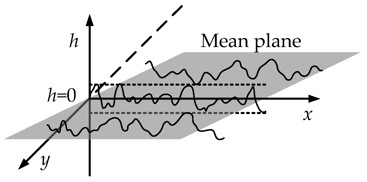
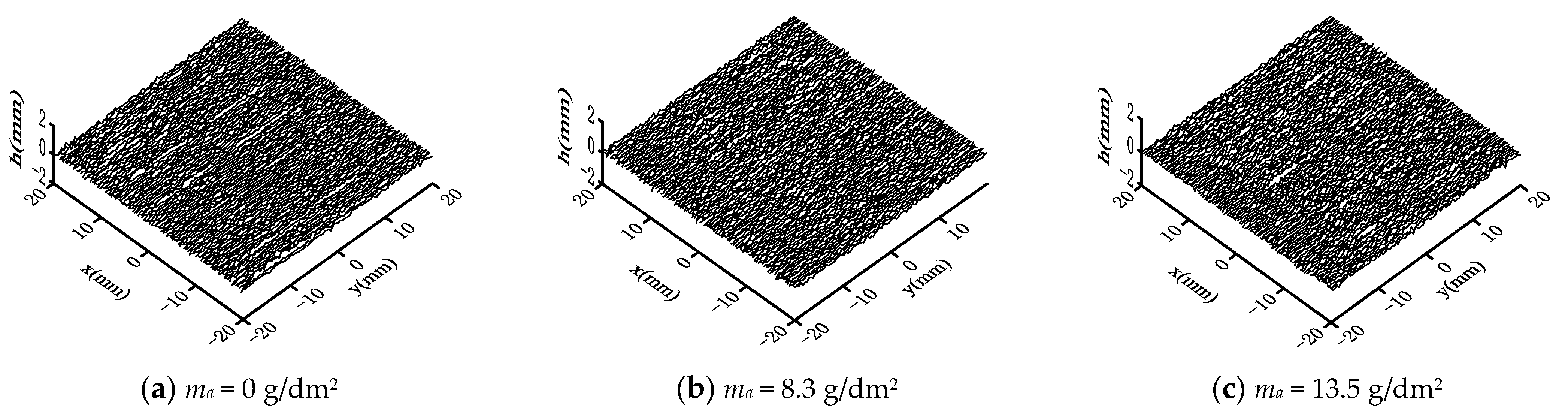
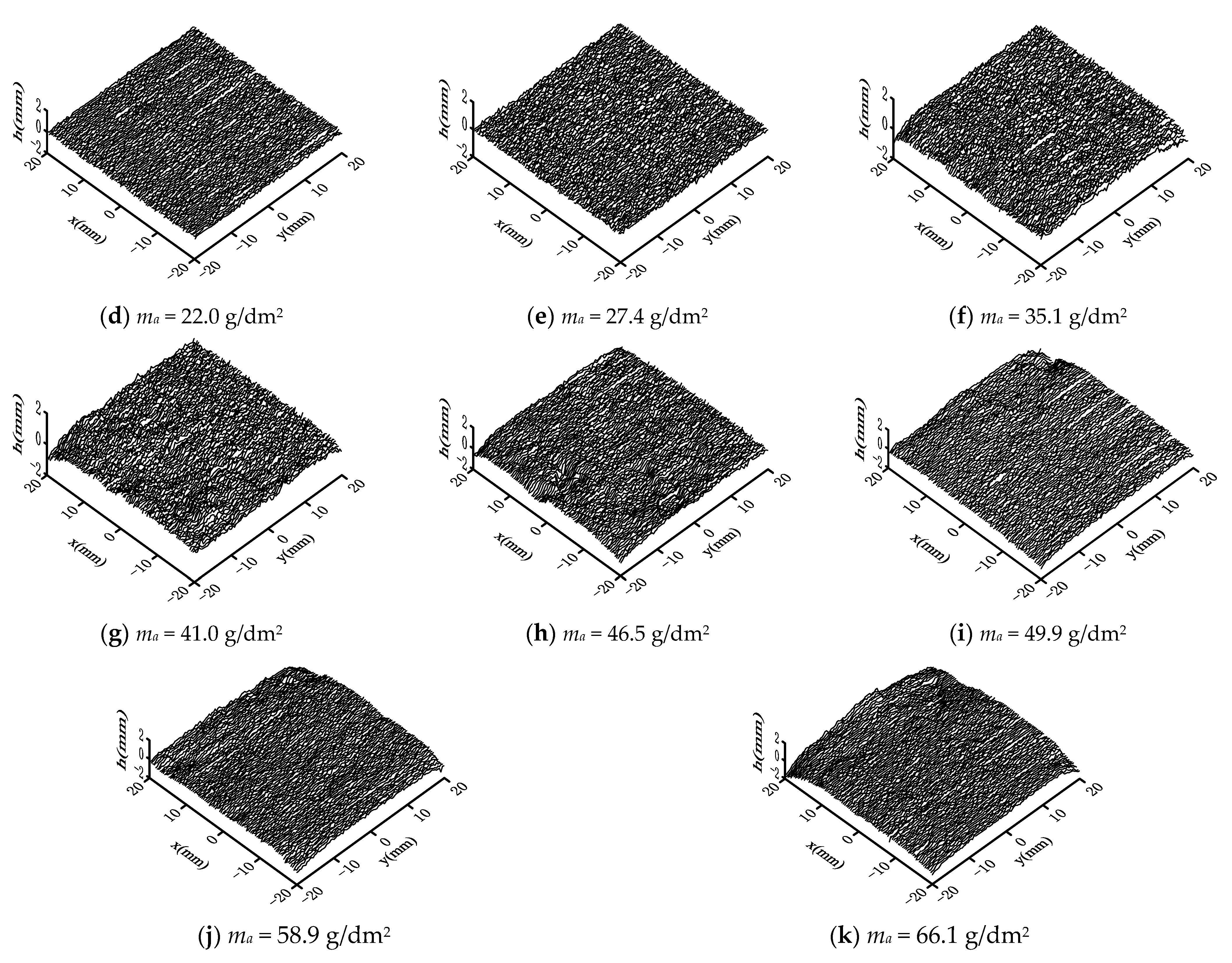
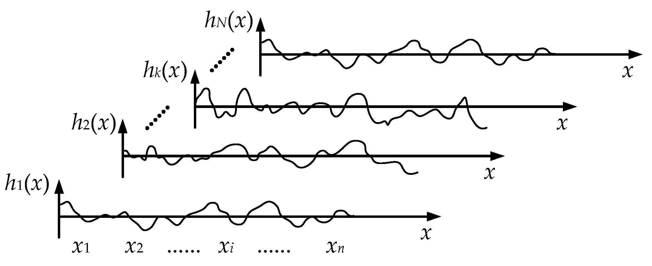
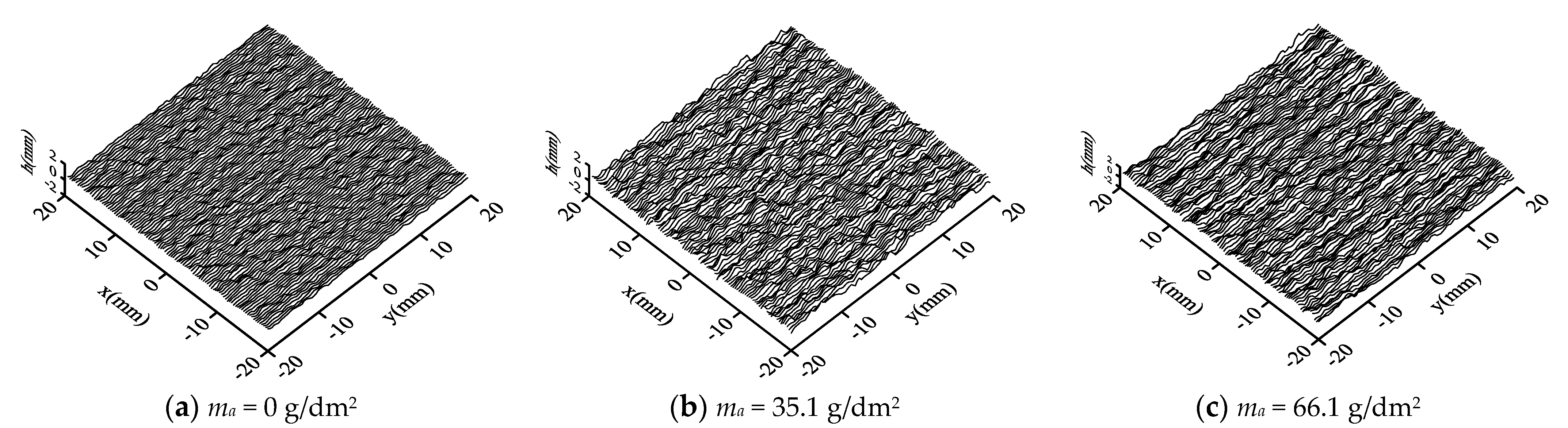
3.1. Surface Topography

To investigate the surface characteristic of corroded samples, a binocular laser scanner is employed to measure the height data of the surface topography. In order to reduce the measurement error at the edge of the circular samples, the square area with a 40 mm side length at the center of the specimen is chosen to investigate the surface characteristic of corroded steel. As the scanning interval is set as 0.1 mm, there are 401 contour curves in each sample area. Each scanning curve has 401 data points. The data are stored on the computer. The height coordinate of the data is the distance of the corroded sample surface relative to the laser scanner. For the convenience of analysis, by subtracting the mean value of the scanning height, a series of surface height data h(x,y) is obtained, which fluctuates around 0. The schematic diagram of the surface height data is illustrated in Figure 4.

The surface curve maps of the corroded surface are drawn in Figure 5. In Figure 5, the corroded surface is composed of a series of uneven two-dimensional contour curves. When the corrosion degree is light, the fluctuation of two-dimensional contour curves is small. With the increasing corrosion degree, the corroded surface has obvious areas of corrosion pits. The number and size of corrosion pits are increasing. Additionally, the fluctuation of the two-dimensional contour curves also increases gradually.

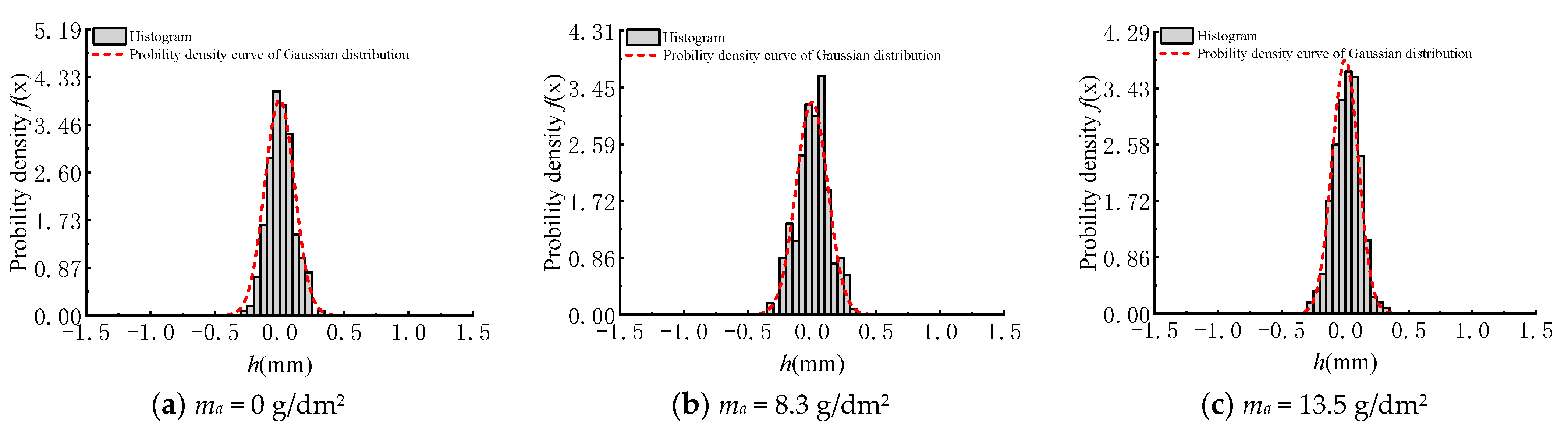
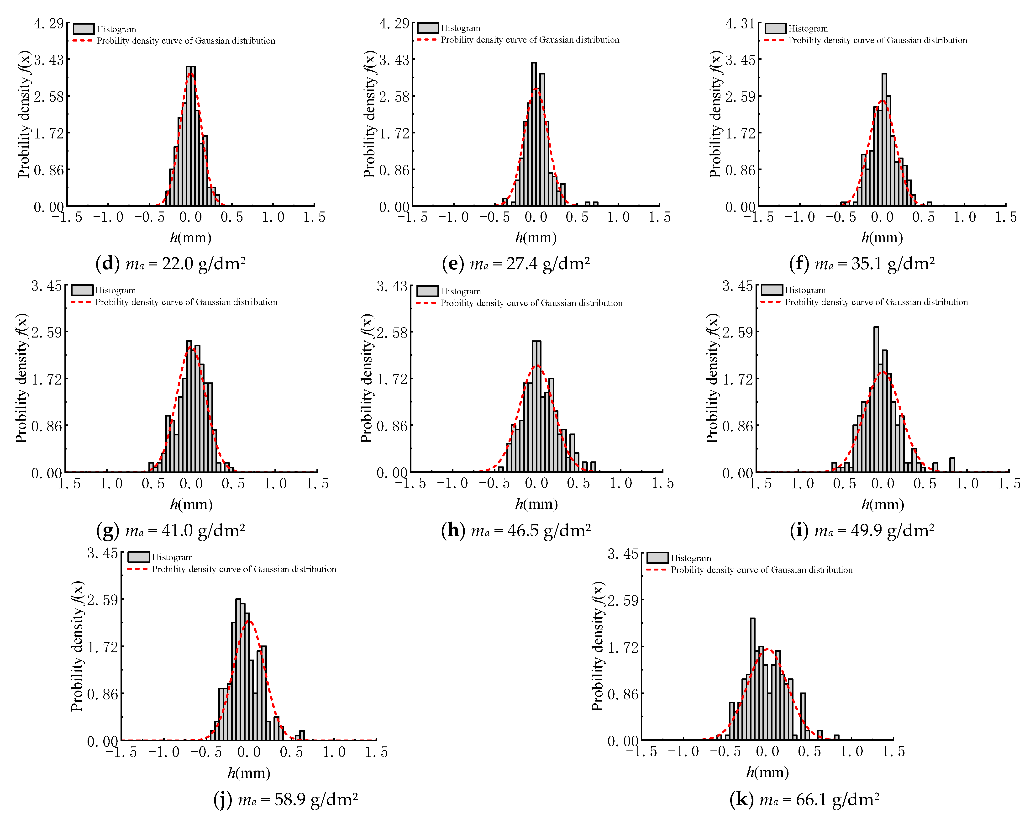
3.2. Surface Height Distribution

In order to analyze the distribution of surface height, the surface height probability density of the two-dimensional contour curve is calculated and plotted in Figure 6. Considering that each sample has 401 contour curves, only one representative two-dimensional contour curve is selected for each sample to draw the histogram of surface height, as shown in Figure 6. It can be found from Figure 6 that the probability density of the two-dimensional contour curve of each sample is almost symmetric on both sides of the surface height of 0 mm. The closer the surface height equals 0, the larger the probability density is. The shape of the histogram of surface height probability density is similar to the probability density curve of the Gaussian distribution.

To prove the surface height of the contour curve follows the Gaussian distribution, based on the probability density function of the Gauss distribution, the mean value and standard deviation of the surface height of contour curve are calculated. The probability density curves following the Gaussian distribution are drawn in Figure 6 with calculated mean value and standard deviation to compare with the histogram of probability density. The probability density function of Gauss distribution can be written as

$$f\left(x;\mu ,\sigma \right)=\frac{1}{\sigma \sqrt{2\pi }}{{\displaystyle \int }}_{-\infty }^x\mathit{exp}\left(-\frac{{\left(x-\mu \right)}^2}{2{\sigma }^2}\right)dx$$

(7)

where µ is the mean value of the surface height of a two-dimensional contour curve, and σ is the standard deviation of the surface height of a two-dimensional contour curve.

The comparison results are shown in Figure 6. It is evident that the height distribution of the two-dimensional contour curve is in accord with the Gaussian distribution form.

The height standard deviation of each two-dimensional contour curve is calculated. The results that corrosion degree ma equals 0 (i.e., no corrosion), 35.1 and 66.1 g/dm² are plotted in Figure 7. It is obvious that the discreteness of the standard deviation is small. Therefore, the mean value of the standard deviation of every two-dimensional contour curve can be adopted as the standard deviation of the surface height of one sample. The variation curve of the standard deviation of surface height of steel samples with different corrosion degrees is drawn in Figure 8. It can be found from this figure that the standard deviation increases with the corrosion degree. It means that the corroded steel surface becomes rougher.

3.3. Development of Mathematical Model

The corroded surface is composed of a series of uneven two-dimensional contour curves. These contour curves can be regarded as experimental results of the sample function of a one-dimensional stochastic process. In previous studies, the Monte Carlo method is the universal method to describe stochastic processes. However, it is usually time-consuming [24]. Shinozuka and Deodatis [25] proposed a spectral representation method to generate one-dimensional, uni-variate, stationary, Gaussian stochastic processes. Considering this method is more efficient than the Monte Carlo method in calculation, the spectral representation method is used to develop the mathematical model of corroded surface in the following.

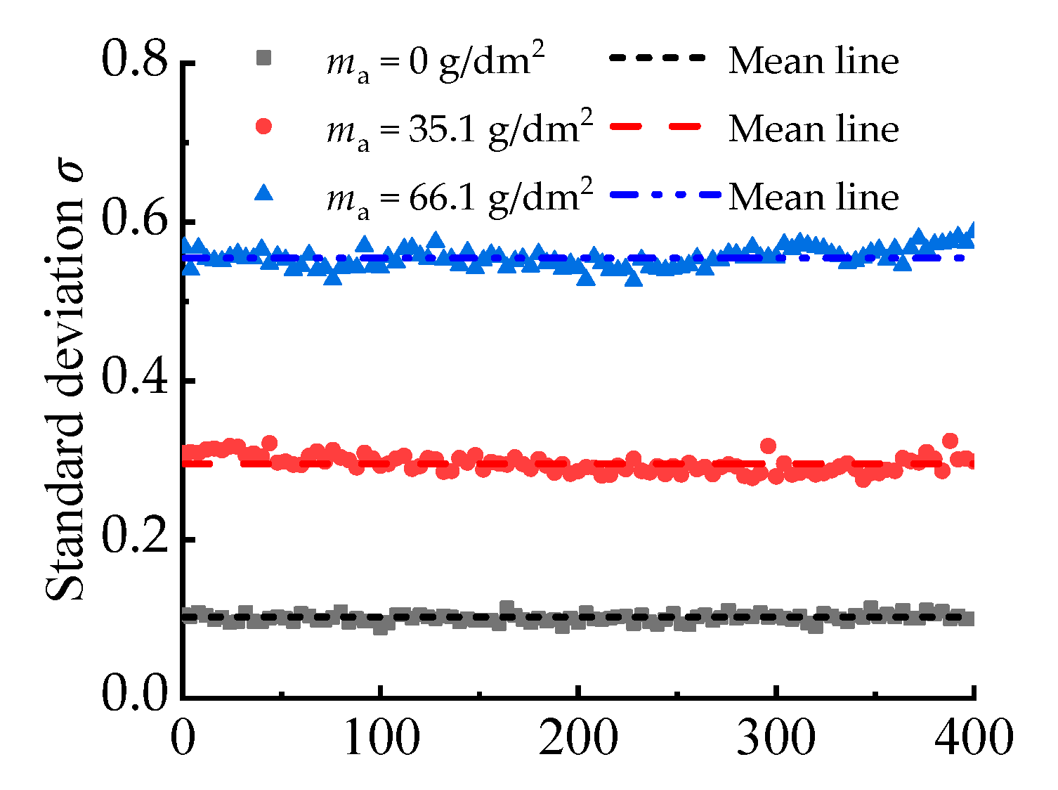
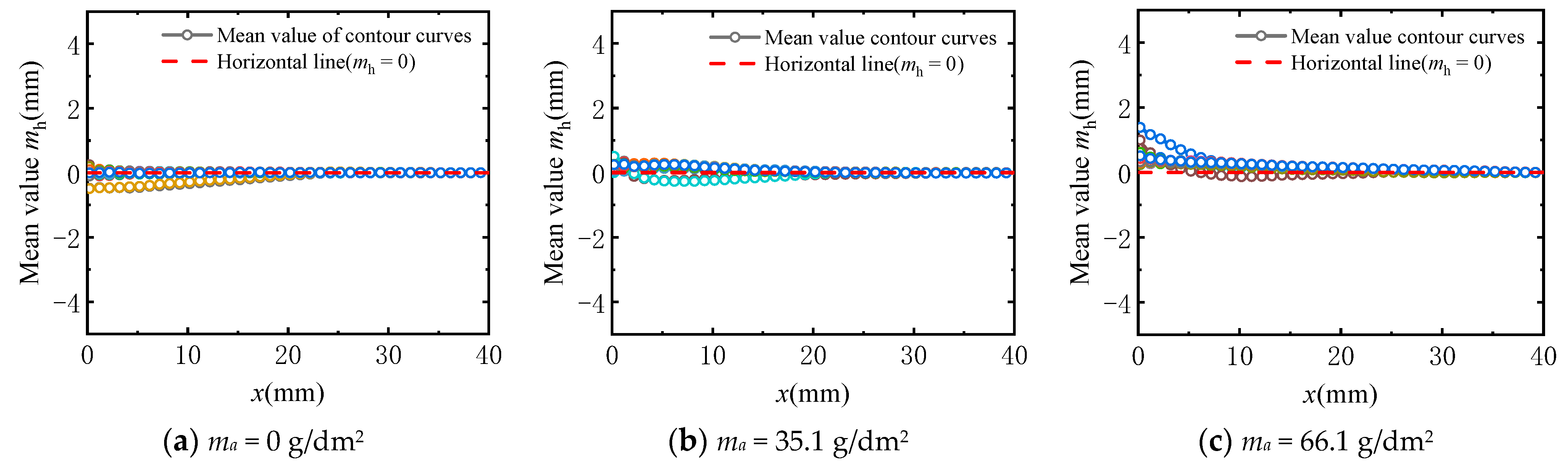
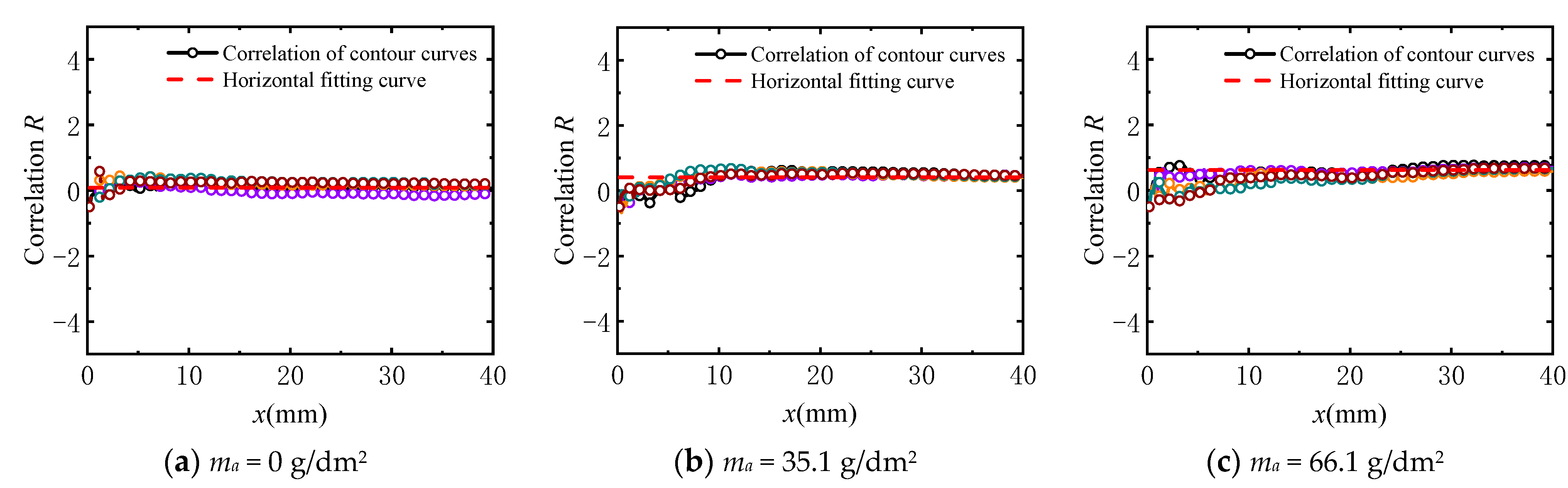
3.3.1. Verification of Stationarity

The corroded surface can be understood as consisting of a series of experimental results of the sample function of the one-dimensional stochastic process. The concept of the stochastic process can be explained in Figure 9. In Figure 9, h_k(x) denotes k-th sample of a one-dimensional stochastic process, where k = 1, 2, …, N. x_i means the i-th data point of any sample of one-dimensional stochastic process along x-axis direction, where I = 1, 2, …, n. Theoretically, when the numbers of samples (N) and data points (n) both tends to be infinity, the precise corroded surface topography can be obtained.

The arbitrary sample of one-dimensional stochastic process consists of a series of stochastic data points along the length x direction, which can be expressed as

$$\left\{h\left(x\right)\right\}=\left\{h\left(x_1\right),h\left(x_2\right),\cdots ,h\left(x_i\right),\cdots ,h\left(x_n\right)\right\}$$

(8)

where x is the coordinate along the length direction; h(x_i) is the surface height of i-th data point of the one-dimensional stochastic process.

In order to develop the mathematical model of the stochastic process with the spectral representation method, the stationary of the one-dimensional stochastic process needs to be verified. According to the above analysis in Section 3.2, the stochastic process {h(x)} is a Gaussian stochastic process, which is also a secondary moment process. For a secondary moment process {h(x)}, if the following conditions are satisfied, the process is a stationary stochastic process.

$$(1)\hspace{1em}\forall x\in X,m_h\left(x\right)=\mathrm{constant};$$

$$(2)\hspace{1em}\forall \tau \in R,x,x+\tau \in X,R_h\left(x,x+\tau \right)=R_h\left(\tau \right).$$

where m_h(x) is the mean value of the stochastic process when the position coordinates equal x; τ is the sampling interval along the length direction; R_h(x,x+τ) is the correlation function when the sampling interval is τ.

The above conditions mean that if the mean value of the stochastic process is a constant independent of position coordinates and the correlation function is a function of sampling interval τ independent of position coordinates, the secondary moment process can be seen as a stationary stochastic process.

Since the two-dimensional contour curves of corroded surface are regarded as a series of samples of a one-dimensional stochastic process, the mean values of surface height of 401 contour curves with different position coordinates are calculated. The variation of mean value with x-coordinate for three corrosion degrees is drawn in Figure 10 as examples. It is obvious that the mean value of the surface height of contour curves is almost equal to zero when the sampling length is greater than 30. When the sampling interval is a unit interval, the correlation function of surface height of 401 contour curves with different position coordinates is calculated. The variation of correlation function with x-coordinate for three corrosion degree are plotted in Figure 11 as an example, too. It can be found that the correlation function tends to be a constant when the sampling length is greater than 30. Figure 10 and Figure 11 show that the mean value and correlation function of surface height of contour curves is independent of position coordinates when the sampling length is greater than 30. Therefore, the contour curves can be regarded as the samples of a one-dimensional stationary Gaussian stochastic process [26,27].

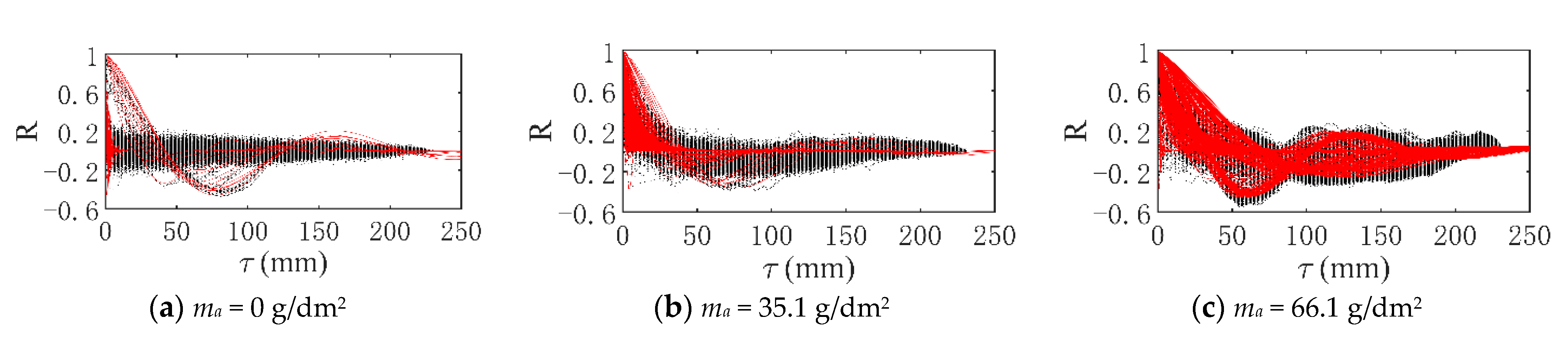
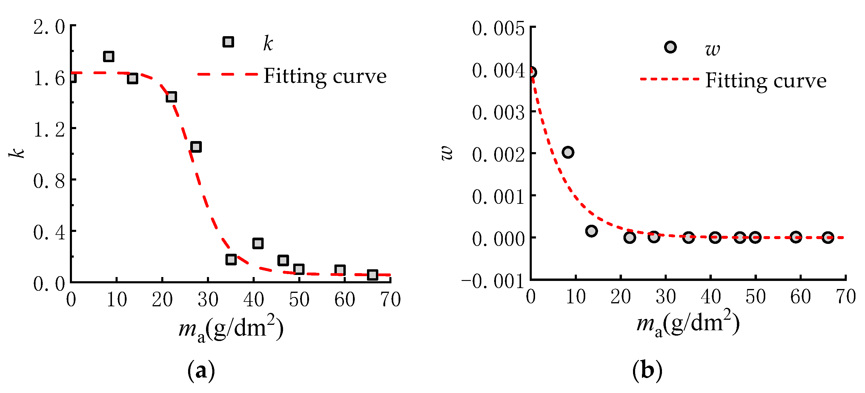
3.3.2. Mathematical Model

After verification of stationarity, the mathematical model of the corroded surface is developed with the spectral representation method in this subsection. According to the study of Shinozuka and Hu [25,28], a one-dimensional stationary stochastic process {h(x)} can be simulated by the following series as N → ∞:

$$h\left(x\right)=\sqrt{2}{\displaystyle \sum }_{n=0}^{N-1}{A}_{n}cos\left(w_{n}x+{\varphi }_n\right)$$

(9)

where

$$A_n={\left(2S_h\left(w_n\right)\Delta w\right)}^{1/2},n=0,1,2,\dots ,N-1$$

(10)

$$w_n=n\times △w,n=0,1,2,\dots ,N-1$$

(11)

$$\Delta w=\frac{w_n}{N}$$

(12)

and

A₀ = 0 or S_h(w₀ = 0) = 0

(13)

In Equation (9), w_n represents an upper cut-off frequency beyond which the power spectral density function S_h(w_n) can be assumed to be zero. Φ_n is an independent random phase angle uniformly distributed in the range [0,2π]. The stochastic process {h(x)} is periodic with period T₀:

$$T_0=2\pi /\Delta w$$

(14)

For a one-dimensional stationary stochastic process, the power spectrum function S_h(w) and the autocorrelation function R(τ) are a pair of Fourier transform pairs. They have the form as

$$\{\begin{array}{c}{S}_h\left(w\right)={{\displaystyle \int }}_{-\infty }^{+\infty }R\left(\tau \right)e^{-iw\tau }d\tau \\ R\left(\tau \right)=\frac{1}{2\pi }{{\displaystyle \int }}_{-\infty }^{+\infty }{S}_h\left(w\right)e^{iw\tau }dw\end{array}$$

(15)

Equation (15) is called the Wiener–Khintchine formula, which reveals the connection between the statistical law describing the stationary process from the time perspective and the statistical law describing the stationary process from the frequency perspective.

Since S_h(w) and R(τ) are even functions, Equation (15) could be rewritten in the form of Equation (16) using Euler’s formula as

$$\{\begin{array}{c}{S}_h\left(w\right)=2{{\displaystyle \int }}_0^{+\infty }R\left(\tau \right)e^{iw\tau }d\tau \\ R\left(\tau \right)=\frac{1}{\pi }{{\displaystyle \int }}_0^{+\infty }{S}_h\left(w\right)e^{iw\tau }dw\end{array}$$

(16)

The autocorrelation function of surface height is an important parameter to characterize the variation of the parameter space points. The cosine exponential model is always used to fit the autocorrelation function [29,30]. The fitting formula has the form as

$$R\left(\tau \right)=exp\left(-k\left|\tau \right|\right)\left(cos\left(w\tau \right)\right)$$

(17)

where τ is the sampling interval; k and w are the parameters of the fitting formula.

If the unit sampling interval is τ₀, the sampling interval can be expressed as j·τ₀. Therefore, the different values of j are selected, and the length of the sampling interval is different. For two-dimensional contour curves, the maximum sampling interval is the length of the contour curve along the length direction.

According to the definition of autocorrelation function [31], the autocorrelation function of surface height of two-dimensional contour curves could be calculated as

$$\begin{array}{l}R\left(\tau \right)=R\left(i\cdot {\tau }_0\right)=E\left[h\left(x\right)h\left(x+\tau \right)\right]\\ ={\displaystyle {\int }_{-\infty }^{+\infty }{x}_1{x}_2{f}_2\left(x_1,x_2;\tau \right)d{x}_{1}d{x}_2=\frac{1}{n-i}{\displaystyle \sum _{k=0}^{n-i}h\left(x_k\right)h\left(x_{k+i}\right)}}\end{array}$$

(18)

Based on Equations (17) and (18), the autocorrelation function of surface height of two-dimensional contour curves is calculated and fitted. The fitting diagrams for three corrosion degrees are shown in Figure 12. In Figure 12, the black points are the calculated values of the autocorrelation function of contour curves. The red curves are the fitting curves fitted with Equation (17).

It can be found from Figure 12 that the autocorrelation function varies with the increase in corrosion degree. For the statistical analysis of the parameters k and w of the fitting curves, it is found that the mean values of parameters k and w of all fitting curves for every sample have an S-logistic function form and exponential function form, respectively, with the increasing of corrosion degree. Therefore, the S-logistic function and exponential function are used to fit the variations of parameters k and w, respectively. The fitting formulas are given as

$$k=0.05665+\frac{1.57188}{1+{\left(m_a/27.5374\right)}^{8.14368}}$$

(19)

$$w=0.00402\times {0.3864}^{\left(m_a/6.6195\right)}$$

(20)

The fitting diagrams of parameters k and w are plotted in Figure 13. It can be found that the parameter k decreases slowly when corrosion degree ma is smaller than 20 g/dm². The rate of reduction increases when corrosion degree ma increases from 20 to 40 g/dm². The parameter k tends to be stable when corrosion degree m_a is larger than 40 g/dm². The variation of parameter w differs from that of parameter k. Parameter w decreases when corrosion degree ma is smaller than 20 g/dm². Then with the increasing of corrosion degree m_a, parameter w tends to be stable.

Combining Equations (17), (19) and (20), the function for the variation of the autocorrelation function with the corrosion degree m_a can be obtained. According to Equation (16), the Fourier transform of the autocorrelation function is the power spectrum function. Therefore, the function for the variation of the power spectrum function with the corrosion degree ma can be expressed as

$$\{\begin{array}{l}{S}_h\left(w\right)=2{\displaystyle {\int }_0^{+\infty }R\left(\tau \right)e^{iw\tau }d\tau }\\ R\left(\tau \right)=\exp (-k|\tau |)\left(\cos \left(w\tau \right)\right)\\ k=0.05665+\frac{1.57188}{1+{\left(m_a/27.5374\right)}^{8.14368}}\\ w=0.00402\times {0.3864}^{\left(m_a/6.6195\right)}\end{array}$$

(21)

Based on Equations (9)–(10), the stochastic function of one-dimensional stationary stochastic process {h(x)} can be written as

$$h\left(x\right)=\sqrt{2}{\displaystyle \sum _{n=0}^{N-1}\sqrt{2S_h\left(w_n\right)\Delta w}\cos \left(w_{n}x+{\varphi }_n\right)}$$

(22)

Substituting Equation (21) into Equation (22), the stochastic process {h(x)} with different corrosion degrees can be simulated.

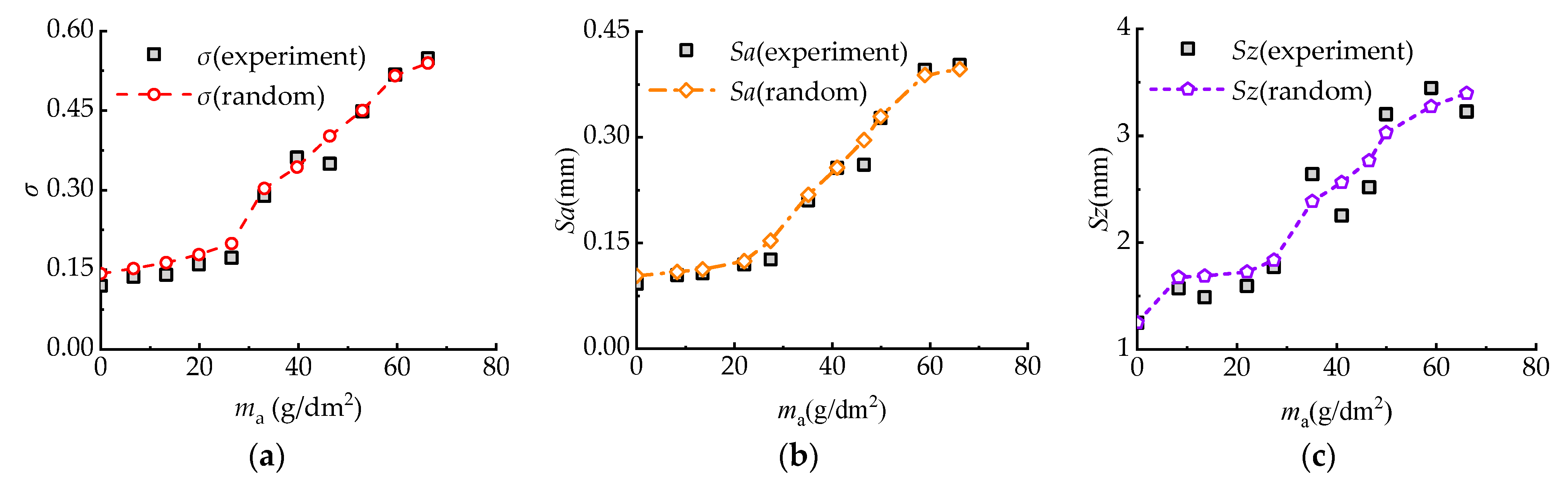
3.4. Stochastic Result Validation

Based on the above mathematical model of one-dimension stochastic process, the two-dimensional contour curves of corroded surfaces with different corrosion degrees can be generated, as shown in Figure 14. These sample curves fluctuate around 0. With the increase in corrosion degree, the fluctuation amplitude of the sample curve increases. It represents the corroded surface becoming rougher.

In order to prove the reliability of the mathematical model, the standard deviation σ, arithmetic mean height S_a and maximum height S_z of randomly generated two-dimensional contour curves and experimental samples are compared [32,33]. Standard deviation σ represents the dispersion degree of surface height of the two-dimensional contour curve. It can be calculated as

$$\sigma =\sqrt{\frac{{\displaystyle \sum _{i=1}^{n}h{\left(x_i\right)}^2}}{n}}$$

(23)

where n is the number of points of the two-dimensional contour curve; h(x_i) is the surface height when the coordinate is x_i.

The arithmetic mean height S_a is the arithmetic mean of the surface offset within the sampling area, which reflects the fluctuation of surface height. The calculation formula is expressed as

The maximum height S_z is the distance between the maximum surface peak height S_p and the maximum surface valley depth S_v within the sampling range. The calculation formula is written as

S_z = S_p − S_v

(24)

where S_p is the maximum surface peak height; S_v is the maximum surface valley depth.

The comparison results are shown in Figure 15. It can be found that the standard deviation, arithmetic mean height and maximum height of randomly generated two-dimensional contour curves are similar to those of the experiment samples. It proves that the mathematical model of corroded surface topography is reliable. The randomly generated two-dimensional contour curves can be used to represent the corroded surfaces.

4. Discussion

For any point on the corroded surface, it is crossed by a lot of two-dimensional contour curves. For the convenience of computation, any point on the corroded surface is regarded as the mean value of the height of randomly generated two-dimensional contour curves through that point in x-direction and y-direction. Therefore, the surface height of any point of the corroded surface h(x,y) can be expressed as

$$h\left(x,y\right)=\frac{h\left(x\right)+h\left(y\right)}{2}$$

(25)

$$h\left(x\right)=\sqrt{2}{\displaystyle \sum _{n=0}^{N-1}\sqrt{2S_h\left(w_n\right)\Delta w}\cos \left(w_{n}x+{\varphi }_{nx}\right)}$$

(26)

$$h\left(y\right)=\sqrt{2}{\displaystyle \sum _{n=0}^{N-1}\sqrt{2S_h\left(w_n\right)\Delta w}\cos \left(w_{n}y+{\varphi }_{ny}\right)}$$

(27)

According to the sum to product formula of trigonometric functions, Equation (25) can be written as Equation (29).

$$\cos \alpha +\cos \beta =2\cos \frac{\alpha +\beta }{2}\cos \frac{\alpha -\beta }{2}$$

(28)

$$\begin{array}{l}h\left(x,y\right)=\frac{h\left(x\right)+h\left(y\right)}{2}\\ =\sqrt{2}\left[\begin{array}{l}{\displaystyle \sum _{n=0}^{N-1}\sqrt{2S_h\left(w_n\right)\Delta w}\cos \left(\frac{\left(w_{n}x+w_{n}y\right)+\left({\varphi }_{nx}+{\varphi }_{ny}\right)}{2}\right)}\\ \cos \left(\frac{\left(w_{n}x-w_{n}y\right)+\left({\varphi }_{nx}-{\varphi }_{ny}\right)}{2}\right)\end{array}\right]\end{array}$$

(29)

Based on the mathematical model of a three-dimensional surface, the stochastic surface topography of different corrosion degrees is generated, as shown in Figure 16. It is evident that the corroded surface is rough, and corrosion pits appear randomly on the surface. In fact, the three-dimensional surface can be regarded as a two-dimensional stochastic field based on the position coordinates. Generating a three-dimensional surface with the mathematical model of a one-dimensional stochastic process is a simplified method. Compared with the simplified method in past works that assumes the corrosion pit is cylindrical shaped pits or conical pits, the reconstructed surface topography is more effective in describing the property of corroded steel surface [15,16].

5. Conclusions

In this paper, the corrosion characteristics in the submarine soil environment of steel structure are studied by electrochemical accelerated corrosion experiments. The corrosion characteristics are summarized through the analysis of electrochemical reactions and mass loss. The variation rules of surface topography of corroded steel samples are investigated by scanning tests. The following conclusion can be drawn:

(1)

The mass loss per unit area increases linearly with the corrosion time. Based on Faraday’s law, the experimental value and theoretical value of mass loss are compared. The result indicates that when the corrosion time is less than 3 h, the mass loss rates of two electrochemical reaction processes during which the corrosion product is divalent iron and trivalent iron, respectively, are similar. With the increasing corrosion time, the corrosion products of experiments are mainly trivalent iron.

(2)

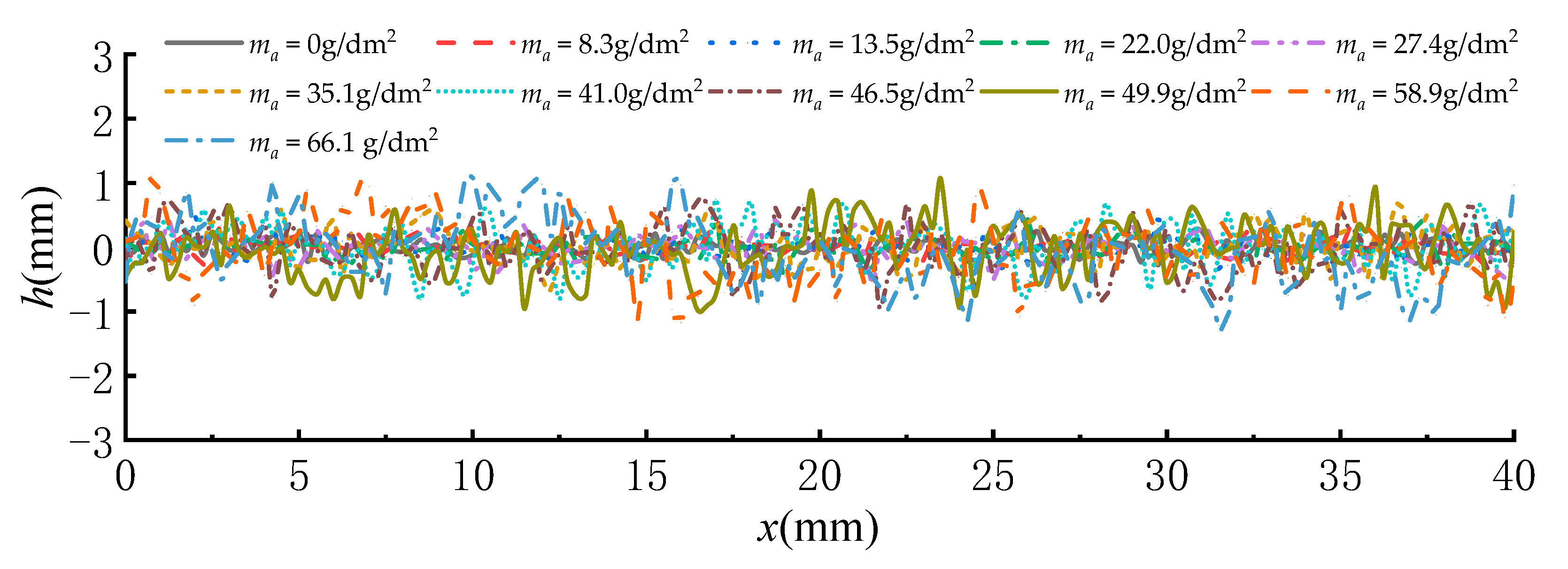
With the increasing corrosion degree, the corroded steel surface becomes rougher, and the number and size of corrosion pits increase. The height of surface two-dimensional contour curves under different corrosion degrees obeys the Gaussian distribution.

Based on the spectral representation method, a mathematical model is developed for a one-dimensional profile of a corroded steel surface. The reliability of the mathematical model is proved by comparing the standard deviation, arithmetic mean height and maximum height of reconstructed samples with those of experimental samples. By assuming that the height of any point on the corroded surface equals the mean value of heights of randomly generated two-dimensional contour curves through that point along x-direction and y-direction, the three-dimensional surface can be reconstructed. The mathematical model can be adapted to reconstruct the surface topography of steel with different corrosion degrees in the following research on the shearing behavior of soil-corroded steel interface.

References

1. Sathish, T.; Mohanavel, V.; Arunkumar, T.; Raja, T.; Rashedi, A.; Alarifi, I.M.; Badruddin, I.A.; Algahtani, A.; Afzal, A. Investigation of Mechanical Properties and Salt Spray Corrosion Test Parameters Optimization for AA8079 with Reinforcement of TiN + ZrO2. Materials 2021, 14, 5260. [Google Scholar] [CrossRef] [PubMed]
2. Momber, A. Corrosion and corrosion protection of support structures for offshore wind energy devices (OWEA). Mater. Corros. 2010, 62, 391–404. [Google Scholar] [CrossRef]
3. Kirchgeorg, T.; Weinberg, I.; Hörnig, M.; Baier, R.; Schmid, M.; Brockmeyer, B. Emissions from corrosion protection systems of offshore wind farms: Evaluation of the potential impact on the marine environment. Mar. Pollut. Bull. 2018, 136, 257–268. [Google Scholar] [CrossRef] [PubMed]
4. Kovendhan, M.; Kang, H.; Jeong, S.; Youn, J.-S.; Oh, I.; Park, Y.-K.; Jeon, K.-J. Study of stainless steel electrodes after electrochemical analysis in sea water condition. Environ. Res. 2019, 173, 549–555. [Google Scholar] [CrossRef]
5. James, M.; Hattingh, D. Case studies in marine concentrated corrosion. Eng. Fail. Anal. 2015, 47, 1–15. [Google Scholar] [CrossRef]
6. Lv, K.; Xu, S.; Liu, L.; Wang, X.; Li, C.; Wu, T.; Yin, F. Comparative Study on the Corrosion Behaviours of High-Silicon Chromium Iron and Q235 Steel in a Soil Solution. Int. J. Electrochem. Sci. 2020, 5193–5207. [Google Scholar] [CrossRef]
7. Wei, B.; Qin, Q.; Bai, Y.; Yu, C.; Xu, J.; Sun, C.; Ke, W. Short-period corrosion of X80 pipeline steel induced by AC current in acidic red soil. Eng. Fail. Anal. 2019, 105, 156–175. [Google Scholar] [CrossRef]
8. Karagah, H.; Shi, C.; Dawood, M.; Belarbi, A. Experimental investigation of short steel columns with localized corrosion. Thin-Walled Struct. 2015, 87, 191–199. [Google Scholar] [CrossRef]
9. Liu, X.; Nanni, A.; Silva, P.F. Rehabilitation of Compression Steel Members Using FRP Pipes Filled with Non-Expansive and Expansive Light-Weight Concrete. Adv. Struct. Eng. 2005, 8, 129–142. [Google Scholar] [CrossRef]
10. Wang, K.; Zhao, M.-J. Mathematical Model of Homogeneous Corrosion of Steel Pipe Pile Foundation for Offshore Wind Turbines and Corrosive Action. Adv. Mater. Sci. Eng. 2016, 2016, 9014317. [Google Scholar] [CrossRef] [Green Version]
11. Wang, K.; Li, Z.; Zhao, M. Mechanism of Localized Corrosion of Steel Pipe Pile Foundation for Offshore Wind Turbines and Corrosive Action. Open Civ. Eng. J. 2016, 10, 685–694. [Google Scholar] [CrossRef] [Green Version]
12. Yamamoto, N.; Ikegami, K. A Study on the Degradation of Coating and Corrosion of Ship’s Hull Based on the Probabilistic Approach. J. Offshore Mech. Arct. Eng. 1998, 120, 121–128. [Google Scholar] [CrossRef]
13. Akpan, U.O.; Koko, T.; Ayyub, B.; Dunbar, T. Risk assessment of aging ship hull structures in the presence of corrosion and fatigue. Mar. Struct. 2002, 15, 211–231. [Google Scholar] [CrossRef]
14. Guo, J.; Wang, G.; Ivanov, L.; Perakis, A.N. Time-varying ultimate strength of aging tanker deck plate considering corrosion effect. Mar. Struct. 2008, 21, 402–419. [Google Scholar] [CrossRef]
15. Jiang, X.; Soares, C.G. Ultimate capacity of rectangular plates with partial depth pits under uniaxial loads. Mar. Struct. 2012, 26, 27–41. [Google Scholar] [CrossRef]
16. Ahmmad, M.; Sumi, Y. Strength and deformability of corroded steel plates under quasi-static tensile load. J. Mar. Sci. Technol. 2009, 15, 1–15. [Google Scholar] [CrossRef]
17. Nakai, T.; Matsushita, H.; Yamamoto, N. Effect of pitting corrosion on local strength of hold frames of bulk carriers (2nd Report)—Lateral-distortional buckling and local face buckling. Mar. Struct. 2004, 17, 612–641. [Google Scholar] [CrossRef]
18. Nakai, T.; Matsushita, H.; Yamamoto, N. Effect of pitting corrosion on the ultimate strength of steel plates subjected to in-plane compression and bending. J. Mar. Sci. Technol. 2006, 11, 52–64. [Google Scholar] [CrossRef]
19. Chen, J.; Fu, C.; Ye, H.; Jin, X. Corrosion of steel embedded in mortar and concrete under different electrolytic accelerated corrosion methods. Constr. Build. Mater. 2020, 241, 117971. [Google Scholar] [CrossRef]
20. Li, Y.; Xu, C.; Zhang, R.H.; Liu, Q.; Wang, X.H.; Chen, Y.C. Effects of Stray AC Interference on Corrosion Behavior of X70 Pipeline Steel in a Simulated Marine Soil Solution. Int. J. Electrochem. Sci. 2017, 1829–1845. [Google Scholar] [CrossRef]
21. Xu, Z.; Du, Y.; Qin, R.; Zhang, H. Study of Corrosion Behavior of X80 Steel in Clay Soil with Different Water Contents under HVDC Interference. Int. J. Electrochem. Sci. 2020, 3935–3954. [Google Scholar] [CrossRef]
22. Wang, X.; Song, X.; Chen, Y.; Wang, Z.; Zhang, L. Corrosion Behavior of X70 and X80 Pipeline Steels in Simulated Soil Solution. Int. J. Electrochem. Sci. 2018, 13, 6436–6450. [Google Scholar] [CrossRef]
23. Su, X.; Yin, Z.; Cheng, Y.F. Corrosion of 16Mn Line Pipe Steel in a Simulated Soil Solution and the Implication on Its Long-Term Corrosion Behavior. J. Mater. Eng. Perform. 2012, 22, 498–504. [Google Scholar] [CrossRef]
24. Shinozuka, M.; Deodatis, G. Simulation of Multi-Dimensional Gaussian Stochastic Fields by Spectral Representation. Appl. Mech. Rev. 1996, 49, 29–53. [Google Scholar] [CrossRef]
25. Shinozuka, M.; Deodatis, G. Simulation of Stochastic Processes by Spectral Representation. Appl. Mech. Rev. 1991, 44, 191–204. [Google Scholar] [CrossRef]
26. Liu, Z.; Liu, W.; Peng, Y. Random function based spectral representation of stationary and non-stationary stochastic processes. Probabilistic Eng. Mech. 2016, 45, 115–126. [Google Scholar] [CrossRef]
27. Hu, Y.; Tonder, K. Simulation of 3-D random rough surface by 2-D digital filter and fourier analysis. Int. J. Mach. Tools Manuf. 1992, 32, 83–90. [Google Scholar] [CrossRef]
28. Hu, B.; Schiehlen, W. On the simulation of stochastic processes by spectral representation. Probabilistic Eng. Mech. 1997, 12, 105–113. [Google Scholar] [CrossRef]
29. Uzielli, M.; Vannucchi, G.; Phoon, K.K. Random field characterisation of stress-nomalised cone penetration testing parameters. Geotechnique 2005, 55, 3–20. [Google Scholar] [CrossRef]
30. Phoon, K.-K.; Quek, S.T.; An, P. Identification of Statistically Homogeneous Soil Layers Using Modified Bartlett Statistics. J. Geotech. Geoenvironmental Eng. 2003, 129, 649–659. [Google Scholar] [CrossRef]
31. Manesh, K.; Ramamoorthy, B.; Singaperumal, M. Numerical generation of anisotropic 3D non-Gaussian engineering surfaces with specified 3D surface roughness parameters. Wear 2010, 268, 1371–1379. [Google Scholar] [CrossRef]
32. Gathimba, N.; Kitane, Y.; Yoshida, T.; Itoh, Y. Surface roughness characteristics of corroded steel pipe piles exposed to marine environment. Constr. Build. Mater. 2019, 203, 267–281. [Google Scholar] [CrossRef]
33. Xia, M.; Wang, Y.; Xu, S. Study on surface characteristics and stochastic model of corroded steel in neutral salt spray environment. Constr. Build. Mater. 2020, 272, 121915. [Google Scholar] [CrossRef]
Figure 1. Electrolytic accelerated corrosion experiment: (a) electrochemical process; (b) experimental system.
Coatings 12 01078 g001
Figure 2. Mass loss per unit area.
Coatings 12 01078 g002
Figure 3. Corrosion mass loss ratio.
Coatings 12 01078 g003
Figure 4. Schematic diagram of surface topography.
Coatings 12 01078 g004
Figure 5. Surface curve maps of corroded steel surface with different corrosion degrees.
Coatings 12 01078 g005aCoatings 12 01078 g005b
Figure 6. Probability density of surface height of two-dimensional contour curve.
Coatings 12 01078 g006aCoatings 12 01078 g006b
Figure 7. Standard deviation of surface height of two-dimensional contour curves.
Coatings 12 01078 g007
Figure 8. Variation of standard deviation σ with corrosion degree ma.
Coatings 12 01078 g008
Figure 9. Schematic diagram of stochastic process on corroded surface.
Coatings 12 01078 g009
Figure 10. Mean value of surface height of two-dimensional contour curves.
Coatings 12 01078 g010
Figure 11. Correlation function of surface height of two-dimensional contour curves.
Coatings 12 01078 g011
Figure 12. Sample autocorrelation function fitting diagram.
Coatings 12 01078 g012
Figure 13. Variation curve of parameters k and w with corrosion degree: (a) parameter k; (b) parameter w.
Coatings 12 01078 g013
Figure 14. Randomly generated two-dimensional contour curves under different corrosion degree.
Coatings 12 01078 g014
Figure 15. Comparison diagrams: (a) standard deviation σ; (b) arithmetic mean height Sa; (c) maximum height Sz.
Coatings 12 01078 g015
Figure 16. Randomly generated corroded surface with different corrosion degrees.
Coatings 12 01078 g016
Publisher’s Note: MDPI stays neutral with regard to jurisdictional claims in published maps and institutional affiliations.