Research on Fault Feature Extraction Method Based on Parameter Optimized Variational Mode Decomposition and Robust Independent Component Analysis

Abstract

The variational mode decomposition mode (VMD) has a reliable mathematical derivation and can decompose signals adaptively. At present, it has been widely used in mechanical fault diagnosis, financial analysis and prediction, geological signal analysis, and other fields. However, VMD has the problems of insufficient decomposition and modal aliasing due to the unclear selection method of modal component k and penalty factor α. Therefore, it is difficult to ensure the accuracy of fault feature extraction and fault diagnosis. To effectively extract fault feature information from bearing vibration signals, a fault feature extraction method based on VMD optimized with information entropy, and robust independent component analysis (RobustICA) was proposed. Firstly, the modal component k and penalty factor α in VMD were optimized by the principle of minimum information entropy to improve the effect of signal decomposition. Secondly, the optimal parameters weresubstituted into VMD, and several intrinsic mode functions (IMFs) wereobtained by signal decomposition. Secondly, the kurtosis and cross-correlation coefficient criteria were comprehensively used to evaluate the advantages and disadvantages of each IMF.And then, the optimal IMFs were selected to construct the observation signal channel to realize the signal-to-noise separation based on RobustICA. Finally, the envelope demodulation analysis of the denoised signal was carried out to extract the fault characteristic frequency. Through the analysis of bearing simulation signal and actual data, it shows that this method can extract the weak characteristics of rolling bearing fault signal and realize the accurate identification of fault. Meanwhile, in the bearing simulation signal experiment, the results of kurtosis value, cross-correlation coefficient, root mean square error, and mean absolute error are 6.162, 0.681, 0.740, and 0.583, respectively. Compared with other traditional methods, better index evaluation value is obtained.

1. Introduction

Rolling bearing is one of the widely used parts in rotating machinery and equipment in the manufacturing system. It widely exists in the power end, transmission end, and execution end. Due to its complex working environment, it is very prone to failure. According to relevant statistics, about 30% of failures in rotating machinery are related to rolling bearings. Therefore, the research on fault diagnosis of rolling bearing is of great significance to ensure the production safety of relevant enterprises. However, in the actual operation process, due to the influence of external noise, receiving distance, and sensor working environment, the fault characteristics of this component are submerged in the interference of intensebackground noise, which has a significantimpact on fault diagnosis.

At present, the bearing fault diagnosis method based on signal processing has experienced three processes: time–domain analysis, frequency domain analysis, and time–frequency domain analysis. Because the fault signal of rolling bearing is non-stationary and nonlinear, the time–frequency domain analysis method is relatively suitable for processing this signal. Since the development of the time–frequency analysis method, the algorithms often used by relevant experts and scholars include Short-time Fourier transform (STFT) [1,2], S-transform [3], Wigner Ville distribution (WVD) [4], wavelet transform (WT) [5,6], etc., singular spectrum decomposition (SSD) [7], spectral kurtosis (SK) [8], morphological filtering (MF) [9], and singular spectrum analysis (SSA) [10], etc. However, these methods havetheir ownlimitations. For example, the window function of STFT is fixed, which is not conducive to the analysis of non-stationary bearing fault signals. The standard deviation of the S-transform in the Gaussian window function is fixed as the reciprocal of the frequency, which makes the time–frequency aggregation of the high-frequency part of the signal not ideal.WVD has good time–frequency aggregation, but there is cross-term interference. Although WT has the time–frequency local analysis ability of adjustable window, the scale of wavelet transform does not have a good corresponding relationship with the frequency of signal. In SK algorithm, how to set the parameters of passband center frequency and resonance bandwidth will affect its application effect. In MF algorithm, it is difficult to effectively select the type and size of the structuring element. In SSA algorithm, the embedding dimension and time delay of phase space reconstruction cannot be set automatically. After continuous development, relevant scholars have proposed many adaptive signal processing methods based on previous research results and applied them to the fault feature extraction of rolling bearing. For example, empirical mode decomposition (EMD) [11], ensemble empirical mode decomposition (EEMD) [12], local mean decomposition (LMD) [13], etc., Jiang et al. [14] proposed a fault feature extraction method combining EMD and 1.5-dimensional spectrum. In this method, the signal components decomposed by EMD are screened and reconstructed Then the reconstructed Hilbert envelope signal is analyzed by a 1.5-dimensional spectrum to obtain the characteristic fault frequency of bearing. The effectiveness of the proposed method is proved by experimental analysis. Fan et al. [15] used EMD and pesudo-Wigner-Ville distribution (PWVD) to convert rolling bearing vibration signals with different fault degrees into contour time–frequency images, then extracted energy distribution values as features, and constructed a fault diagnosis model based onfuzzy c-means (FCM). Experimental results show that this method has high recognition accuracy. Hou et al. [16] proposed a fault diagnosis method composed of EEMD, permutation entropy (PE), and Gath Geva (GG) clustering algorithm to solve the problem that it is difficult to identify the fault type of rolling bearing. Experimental results show that the proposed fault diagnosis method can achieve better clustering results. Liang et al. [17] proposed a fault diagnosis method based on long-term and short-term memory network (LSTM) and LMD, to improve the defects of the LMD method. The results show that the method successfully extracts the characteristic frequencies of rolling bearing. Although the above time–frequency analysis methods have achieved certain results, they are based on the principle of recursive decomposition, so they have not been well solved in the aspects of modal aliasing and endpoint effect. To solve this problem, Dragomiretskiy et al. [18] proposed a new adaptive decomposition method variational modal decomposition. The algorithm makes the decomposition result stable through the construction of the variational problem and is applied to the fault diagnosis of rotating machinery. Ye et al. [19] decomposed the bearing vibration signal by the VMD method and introduced the characteristic capability ratio criterion to screen the qualified signal components for reconstruction. Then, the multi-dimensional features of the signal are extracted and input into the particle swarm optimization (PSO) andsupport vector machine (SVM) classification model for fault diagnosis. The results show that the proposed method has higher recognition accuracy than the existing methods. Li et al. [20] proposed a fault diagnosis method combining VMD and fractional Fourier transform (FRFT) to solve the problem that it is difficult to extract fault features and over decomposition when applying the VMD method to rolling bearing fault diagnosis. By analyzing the results of simulation experiments, the method has a good effect. Xing et al. [21] combined VMD, Tsallis entropy, and fuzzy c-means clustering (FCM) and applied them to fault diagnosis. Through the analysis of the measured vibration signal of rolling bearing, the results show that this method can obtain better results than EMD and LMD methods.

The signal processed by time–frequency analysis contains a lot of noise, which has a specificimpact on the fault feature extraction. Therefore, the signal needs further processing. In recent years, the technology based on blind source separation has become one of the research hotspots. This technology optimizes multiple observation signals according to the principle of statistical independence and decomposes them into several independent components, so as to achieve the purpose of signal enhancement. Robust independent component analysis (RobustICA), as an algorithm with outstanding advantages in blind source separation methods, has been widely used in signal analysis, fault diagnosis, and other fields because of its good effect in signal-to-noise separation effect and calculation efficiency [22,23,24]. Yang et al. [25] proposed a signal noise-reduction method based on the combination of complementary ensemble empirical mode decomposition (CEEMD) and RobustICA to reduce the noise of pipeline blockage signals. Through the processing and analysis of simulation signals and pipeline blockage detection signals, the results verify the effectiveness of the proposed method. Yao et al. [26] studied the noise reduction of internal combustion engine signals by using the combination of Gammatone filter bank and RobustICA. Experiments show that the classification effect of signal and noise obtained by this method is good. Zhao et al. [27] combined EEMD, RobustICA, and Prony algorithms and applied them to the identification of low-frequency oscillation signals in the power system. Experiments show that the proposed method has a strong anti-interference ability and can effectively suppress noise.

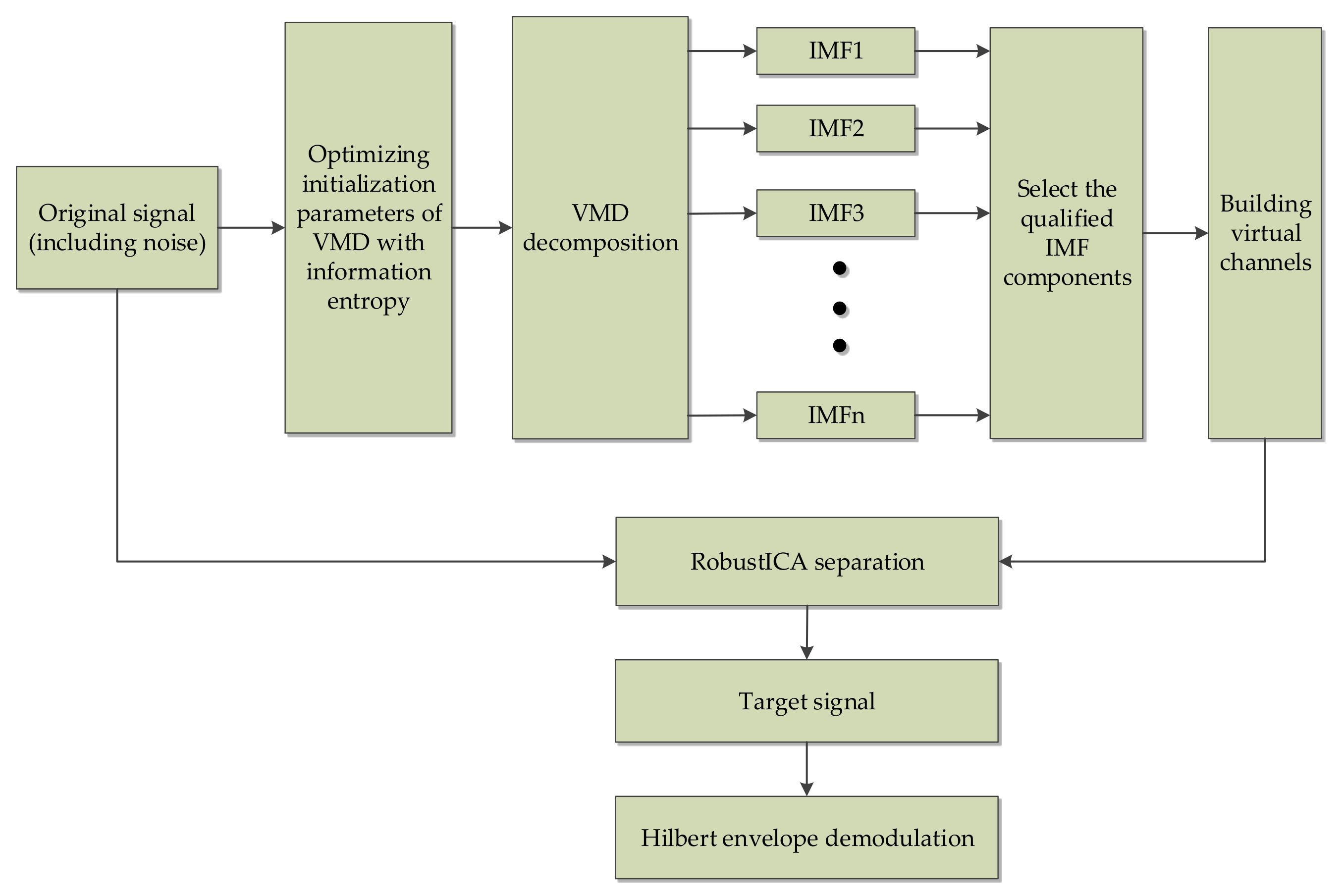
In this paper, a fault feature extraction method based on VMD optimized with information entropy and RobustICA is proposed. Firstly, the fault signal is decomposed by VMD, and the number of modal components k and penalty parameters α are selected according to the optimization principle of minimum information entropy. Then, the optimal parameters are substituted into VMD and the signal decomposition operation is carried out. Secondly, the signal components are filtered through the constructed signal component screening criteria, and the observation signal channel is constructed, so as to realize the signal-to-noise separation based on RobustICA. Finally, the denoised signal is demodulated by Hilbert envelope, and the fault characteristic frequency is extracted.

The main contributions of this paper are summarized as follows:

(1)

A method of optimizing VMD by information entropy is proposed to set initialization parameters so that VMD can adaptively expand signal decomposition;

(2)

In this study, kurtosis and cross-correlation coefficient criteria are comprehensively used to evaluate the advantages and disadvantages of each eigenmode function, and the optimal eigenmode function is selected to construct the observation signal channel, which completes the separation of useful signal and noise signal; and

(3)

The effectiveness and feasibility of the proposed method are verified by experimental analysis using simulation signals and actual bearing data sets.

The structure of this paper is as follows. Section 2 introduces the basic principles of VMD, information entropy, and the RobustICA algorithm. Section 3 introduces the specific implementation process of the fault feature extraction method based on information entropy optimization VMD and RobustICA. In Section 4, the stimulation signal is experimentally studied by using the proposed method. In Section 5, the effect of the method is further verified by the actual bearing fault signal experiment. Section 6 is the discussion and conclusions.

2. Basic Methods

2.1. VMD

Variational modal decomposition (VMD) is developed by University of California scholars Dragomiretskiy et al., in 2014 [18]. Based on Wiener filtering, this method searches for the optimal solution of the input signal within the framework of variational model. It can adaptively update the center frequency, bandwidth, and corresponding sub signals, and decompose the independent components of the signal from the frequency domain. As a non-recursive signal analysis method, the core idea of the VMD method is to determine the intrinsic mode function (IMF) by solving the variational problem. Therefore, in the VMD algorithm, the IMF component obtained by signal decomposition is different from that in EMD and LMD algorithms. The original signal is non recursively decomposed into several IMF components with limited bandwidth:

$${\mu }_k(t)=A_k(t)\mathrm{c}\mathrm{o}\mathrm{s}[{\varphi }_k(t)]$$

(1)

In the above formula, $A_k(t)$ is the instantaneous amplitude of ${\mu }_k(t)$, and $A_k(t)\ge 0$. ${\varphi }_k(t)$ is phase and ${\varphi }_k(t)\ge 0$. ${\omega }_k(t)$ is the instantaneous phase of ${\mu }_k(t)$.

$${\omega }_k(t)={\varphi }_k\prime (t)=\frac{d{\varphi }_k(t)}{dt}$$

(2)

In the above formula, ${\mu }_k(t)$ can be regarded as a harmonic signal, its amplitude is $A_k(t)$ and its frequency is ${\omega }_k(t)$.

It is assumed that each mode has a limited bandwidth with central frequency, and the central frequency and bandwidth will be updated continuously in the decomposition process. Then the variational problem can be expressed as finding r modal functions ${\mu }_k(t)$ and minimizing the estimated bandwidth forthe sum of all modal functions. The sum of modes is the input signal.VMD algorithm can obtain k discrete modes ${\mu }_k(t) (r\in 1,2, \cdots ,R)$ by decomposing signal X(t). Then, the frequency bandwidth of each modal signal is estimated in the following manner.

(1) Hilbert transform is extended to the modal function, and the marginal spectrum is obtained.

$$\left(\delta (t)+\frac{j}{\pi t}\right)\ast {\mu }_k(t)$$

(3)

(2) Each estimated center band is modulated to the corresponding fundamental band.

$$\left[(\delta (t)+\frac{j}{\pi t})\ast {\mu }_k(t)\right]e^{-j{\omega }_{k}t}$$

(4)

(3) The square L² norm of the demodulated signal gradient is obtained.

$${‖d_t[(\delta (t)+\frac{j}{\pi t})\ast {\mu }_k(t)]e^{-j{\omega }_{k}t}‖}_2^2$$

(5)

By constructing the VMD variational constraint model based on the above formula, the following formula can be formed.

$$\left\{\begin{array}{l}\underset{\left\{{\mu }_k\right\},\left\{{\omega }_k\right\}}{\mathrm{m}\mathrm{i}\mathrm{n}}\left\{{\displaystyle \sum _{k=1}^k\Vert d_t[(\delta (t)+\frac{j}{\pi t})\ast {\mu }_k(t)]e^{-j{\omega }_{k}t}{\Vert }_2^2}\right\}\\ \mathrm{s}.\mathrm{t}. {\displaystyle \sum _{k=1}^k{\mu }_k(t)}=x(t)\end{array}\right.$$

(6)

In the above formula, $\left\{{\mu }_k(t)\right\}=\left\{{\mu }_1,{\mu }_2,{\mu }_3,\cdot \cdot \cdot {\mu }_k\right\}$ is the function set of each mode. $\left\{{\omega }_k\right\}=\left\{{\omega }_1,{\omega }_2,{\omega }_3,\cdot \cdot \cdot {\omega }_k\right\}$ is the central frequency set. $\delta (t)$ is the unit pulse function. $d_t$ is the derivative of the function over time t. s.t. is the constraint. $x(t)$ is the original input signal, where k is the number of decompositions.

By introducing penalty factor and Lagrange multiplication operator b, the constrained model problem in Equation (5) can be transformed into a non-constrained model problem, as in Equation (6).

$$L(\left\{{\mu }_k\right\},\left\{{\omega }_k\right\},\lambda )=\alpha {\displaystyle \sum _{k=1}^k\Vert d_t[(\delta (t)+\frac{j}{\pi t})\ast {\mu }_k(t)]e^{-j{\omega }_{k}t}{\Vert }_2^2}+ {‖x(t) -{\displaystyle \sum _{k=1}^k{\mu }_k(t)}‖}_2^2+\langle \lambda (t),x(t)-{\displaystyle \sum _{k=1}^k{\mu }_k(t)}\rangle$$

(7)

By constantly iteratively searching for the minimum point of Lagrange function L, the original input signal a will be decomposed into k modal functions ${\mu }_k(t)$.

When using VMD decomposition algorithm to adaptively decompose the signal, the decomposition parameters need to be set in advance. Theoretical research shows that the parameters that have a great impact on the decomposition effect mainly include the number of decomposition k and the penalty parameter α. Therefore, setting these two parameters only by experience will bring great errors to the decomposition results of VMD. Among them, the size of k value is directly related to the decomposition effect of VMD. If the value of k is too small, it will lead to under decomposition of the signal, and the resulting signal is not completely decomposed into components. If the value of k is too large, the signal will be decomposed too much, resulting in over decomposition. At the same time, the value of a has a certain impact on the bandwidth of the decomposed component. If the value of a is too small, the bandwidth of the decomposed component will be too large, and some components will include other components. If the value of a is too large, the bandwidth of the decomposed component will be too small, and some components in the decomposed signal may be lost.

2.2. Information Entropy

The concept of entropy originates from thermodynamics and is used to describe the disorder degree of the system. Based on this idea, scholar Shannnon proposed the concept of information entropy [28]. Information entropy is a concept used to measure the amount of information in information theory. When a system is more orderly, the value of information entropy will be smaller. On the contrary, when the disorder degree of the system becomes higher, the value of information entropy will become larger. The calculation formula of information entropy is as follows:

$$\mathrm{G}(x)=-{\displaystyle \sum _{i=1}^{n}P(x_i)\mathrm{l}\mathrm{o}\mathrm{g}P(}{x}_i)$$

(8)

where $P(x_i)$ represents the probability of occurrence of an event $x_i$ in the system, and n represents the number of samples to be analyzed.

2.3. Robust Independent Component Analysis

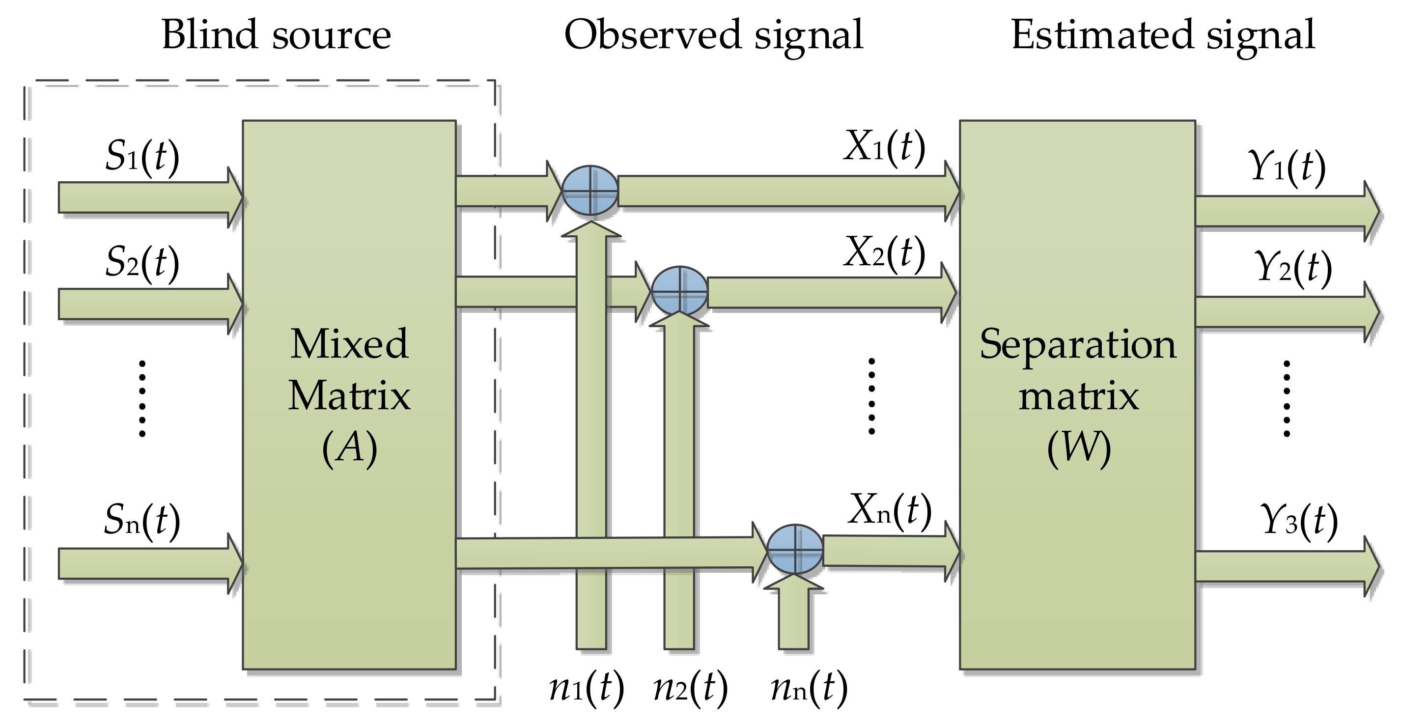
RobustICA algorithm is proposed by Zarzoso et al. [29,30]. Because the observation data used in it does not need whitening preprocessing, it can only meet the condition that its mean value is zero, so the problem of introducing error is avoided. The algorithm realizes the kurtosis optimization by using linear search and algebraic calculation of the global optimal step size. The frame of independent component analysis is shown in Figure 1 [31]. Assuming that the mixed data containing noise is X and the output signal is Y = WX, the kurtosis formula can be expressed as follows:

$$K(W)=\frac{E\left\{\right| Y{|}^4\} -2E^2\{| Y{|}^2\}-\left|E\right\{Y^2\}{|}^2}{E^2\left\{\right|Y{|}^2\}}$$

(9)

where E {·} represents mathematical expectation, W represents separation matrix.

An exact linear search is performed by using the absolute value of kurtosis as the objective function:

$${\mu }_{opt}=\mathrm{a}\mathrm{r}\mathrm{g}\underset{u}{\mathrm{m}\mathrm{a}\mathrm{x}}\left|K(W+\mu g)\right|$$

(10)

The search direction g is usually gradient, namely. $g={\nabla }_{w}K(W)$. It is expressed as follows:

$$g={\nabla }_{w}K(W)= \frac{4}{E^2\left\{\right|Y{|}^2\}}\left\{E\right\{| Y^2|\}YX -E\{YX\left\}E\right\{Y^2\}-\frac{(E\{| Y{|}^4\} -\left|E\right\{Y^2\}{|}^2)E\left\{YX\right\}}{E\left\{\right|Y{|}^2\}}$$

(11)

where K indicates kurtosis. E {·} represents mathematical expectation. ${\nabla }_w$ indicates gradient.

In the process of each iterative operation, the operation steps of RobustICA is as follows:

(1) Find the coefficients of the optimal step polynomial:

$$P(u)={\displaystyle \sum _{k=0}^4{a}_k{u}^k}$$

(12)

(2) Extract the root of the optimal polynomial (12).

(3) In the search direction, the root value that maximizes the kurtosis is selected as the optimal step

$${\mu }_{opt}=\mathrm{a}\mathrm{r}\mathrm{g}\underset{u}{\mathrm{m}\mathrm{a}\mathrm{x}}\left|K(W+\mu g)\right|$$

(13)

(4) Update the separation vector: $W^{+}:W^{+}=W+{\mu }_{opt}g$;

(5) Normalized the separation vector: $W^{+}:W^{+}\leftarrow \frac{W^{+}}{‖W^{+}‖}$;

(6) If there is no convergence, return to Step (1), otherwise the solution of the separation vector is completed.

3. Fault Feature Extraction Based on VMD Optimized with Information Entropy and RobustICA

3.1. Parameter Optimization of VMD

During the working process of rolling bearing, because the inner ring will rotate with the shaft, the pressure of therolling bearing changes periodically. When the rolling bearing fails, the damaged part’s surface will contact other parts and collide. Therefore, it will produce periodic pulse impact. According to this bearing characteristic, the information entropy theory can be used to measure the above changes. When the periodic impact is more uniform, the signal is more orderly, so the value of information entropy will be smaller. Therefore, if the IMF component obtained by VMD decomposition contains more fault information, its performance will be more orderly, and the value of information entropy will be smaller. In this research, envelope entropy is introduced to measure signal sparsity. The envelope entropy of IMF_i(j) component of signal decomposed by VMD algorithm can be expressed as follows:

$$E_i=-{\displaystyle \sum _{j=1}^n{P}_{i,j}\mathrm{l}\mathrm{o}\mathrm{g}{P}_{i,j}}$$

(14)

$$P_{i,j}=a_i(j)/{\displaystyle \sum _{j=1}^n{a}_i(j)}$$

(15)

where, i represents the sequence number of IMF obtained by the decomposition of signal $x(j)$ (i = 1, 2, 3, ⋯). $P_{i,j}$ represents the normalized result of $a_i(j)$. $a_i(j)$ is the envelope signal of signal component IMF_i(j) after Hilbert envelope demodulation. Based on this, this paper adopts the principle of minimum envelope entropy to determine the initialization parameters of VMD.

In parameter optimization, the value of α can be given first, and the optimal value of mode k can be determined based on the principle of minimum envelope entropy. After obtaining the value of k, the optimal value of α is further determined based on the value of k. Its optimization objective can be expressed as shown in Formula (16). Where k_min and k_max represent the minimum and maximum values of the interval range of modal k search, respectively. α_min and α_max represent the minimum and maximum values of the interval range searched by the penalty factor α, respectively. The specific optimization process is shown in Figure 2.

$$\left\{\begin{array}{l}\mathrm{m}\mathrm{i}\mathrm{n}\left\{E\right\}\\ \mathrm{s}.\mathrm{t}. k_{\mathrm{m}\mathrm{i}\mathrm{n}}\le k_z\le k_{\mathrm{m}\mathrm{a}\mathrm{x}}\\ \mathrm{s}.\mathrm{t}. {\alpha }_{\mathrm{m}\mathrm{i}\mathrm{n}}\le {\alpha }_z\le {\alpha }_{\mathrm{m}\mathrm{a}\mathrm{x}}\end{array}\right.$$

(16)

The specific steps are as follows:

(1)

Optimize the modal number k. First, set the initial value of mode number k to 3, and use the default value of 2500 for the penalty factor α. Then, the fault signal is decomposed by VMD, and the envelope entropy of all modes is obtained according to the calculation formula of envelope entropy. According to the calculation results, judge whether the envelope entropy obtainedthe minimum value. If it is the minimum value, select the value at this time as the optimal value. If not, perform k + 1 operation on the value of a modal number, and continue to repeat the above analysis steps until the minimum envelope entropy value is found. Then record the corresponding k value. In this research, the search range of k is from to 3 to 15, and the step size is 1.

(2)

Optimize the penalty factor. Based on the value of k determined in the previous step to further determine the optimal value. The search principle is the same as the previous step. When the minimum envelope entropy value is found, the search is terminated. Otherwise, perform the operation of α + 50 and repeat the above analysis steps until the smallest value of envelope entropy is found, and then record the corresponding value. In this research, the search range of α is set from 100 to 2500, and the step size is 50.

(3)

Based on the optimization results of the first and second steps, the optimal values of k and α are substituted into VMD, and the parameters are initialized. Then perform VMD to get the optimal IMF component.

3.2. Screening Criteria for IMF Components

As a dimensionless parameter, kurtosis is often used for the distribution characteristics of vibration signals. For the IMF signal components obtained by VMD decomposition, when the signal component’s kurtosis value is more prominent, it contains more impact components. At the same time, the cross-correlation coefficient represents the correlation between signals. The greater the correlationcoefficient for the IMF signals components, the more sensitive information it contains. Conversely, the more interference components it contains. Based on this, in the fault signal processing of rolling bearings, this research will comprehensively use the above two criteria to determine which signal components are used to construct the observation signal channel of the RobustICA, and then achieve the purpose of noise reduction. In selecting signal components, the principle adopted is that the correlation number is more significant than 0.3 and the kurtosis value is greater than 3. In this way, it is possible to avoid the problem of using a single index to select only the signal component with the most significantkurtosis value, which leads to the loss of sensitive information of part of the fault signal. The formula for calculating kurtosis and cross-correlation coefficient is as follows:

$${\mathrm{K}\mathrm{u}\mathrm{r}\mathrm{t}\mathrm{o}\mathrm{s}\mathrm{i}\mathrm{s}}_i=\frac{1}{\mu }{\displaystyle \sum _{i=1}^n{(\frac{{\theta }_i-\overline{x}}{\mathcal{l}})}^4}$$

(17)

In the original vibration signal, ${\theta }_i$ and $\overline{x}$ are its actual value and average value. $\mathcal{l}$ is the standard deviation. μ is the number of samples.

$$Correlation=\frac{{\displaystyle \sum _{i=0}^n({\theta }_i-\overline{x})({\delta }_i-\overline{y})}}{\sqrt{{\displaystyle \sum _{i=0}^n{({\theta }_i-\overline{x})}^2{({\delta }_i-\overline{y})}^2}}}$$

(18)

In the original vibration signal, ${\theta }_i$ and $\overline{x}$ its specific value and average value. Meanwhile, ${\delta }_i$ and $\overline{y}$ are the specific and average values of signal ϑ.

3.3. Algorithm Steps and Flow

The specific steps of the fault feature extraction method based on information entropy optimization VMD and RobustICA are as follows. The fault feature extraction process is shown in Figure 3.

(1)

The vibration signal of rolling bearing is collected, and the VMD is optimized by information entropy to find the optimal value of initialization parameter k and α.

(2)

The obtained optimal parameters k and α are substituted into VMD, and the relevant parameters are initialized. Secondly, the signal is decomposed into several IMF components by VMD decomposition.

(3)

Kurtosis criterion and cross-correlation coefficient criterion are comprehensively used to evaluate the advantages and disadvantages of each IMF component, and the optimal IMF component is selected to construct the observation signal channel.

(4)

The observed signal and virtual noise channel signal are separated by RobustICAalgorithm, and the useful signal is obtained.

(5)

Envelope demodulation is performed on the signal after RobustICAnoise reduction, and the fault characteristic frequency is extracted. Then it is compared with the theoretical value of bearing fault characteristics to identify the fault category.

4. Simulations and Comparative Analysis

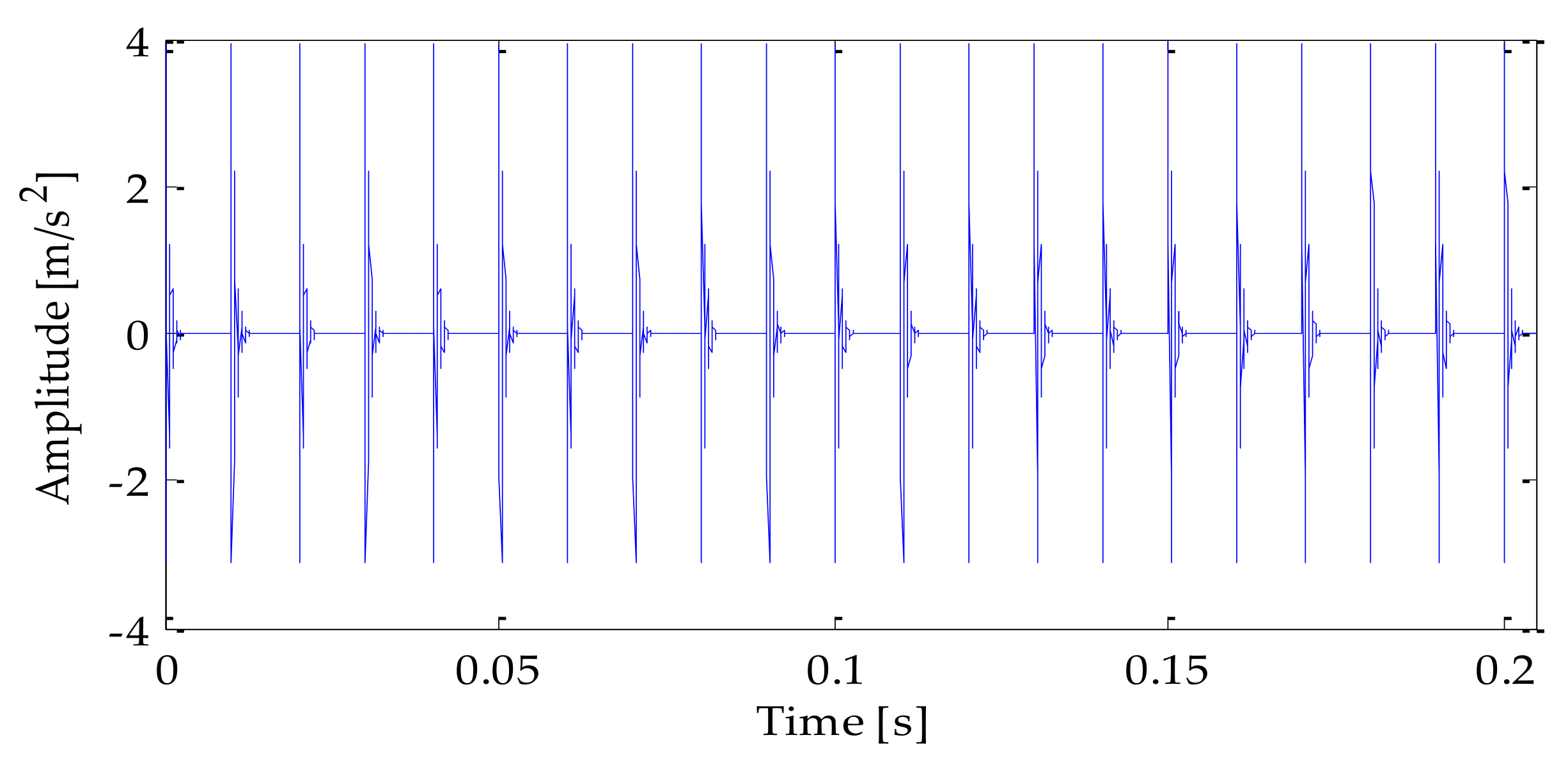
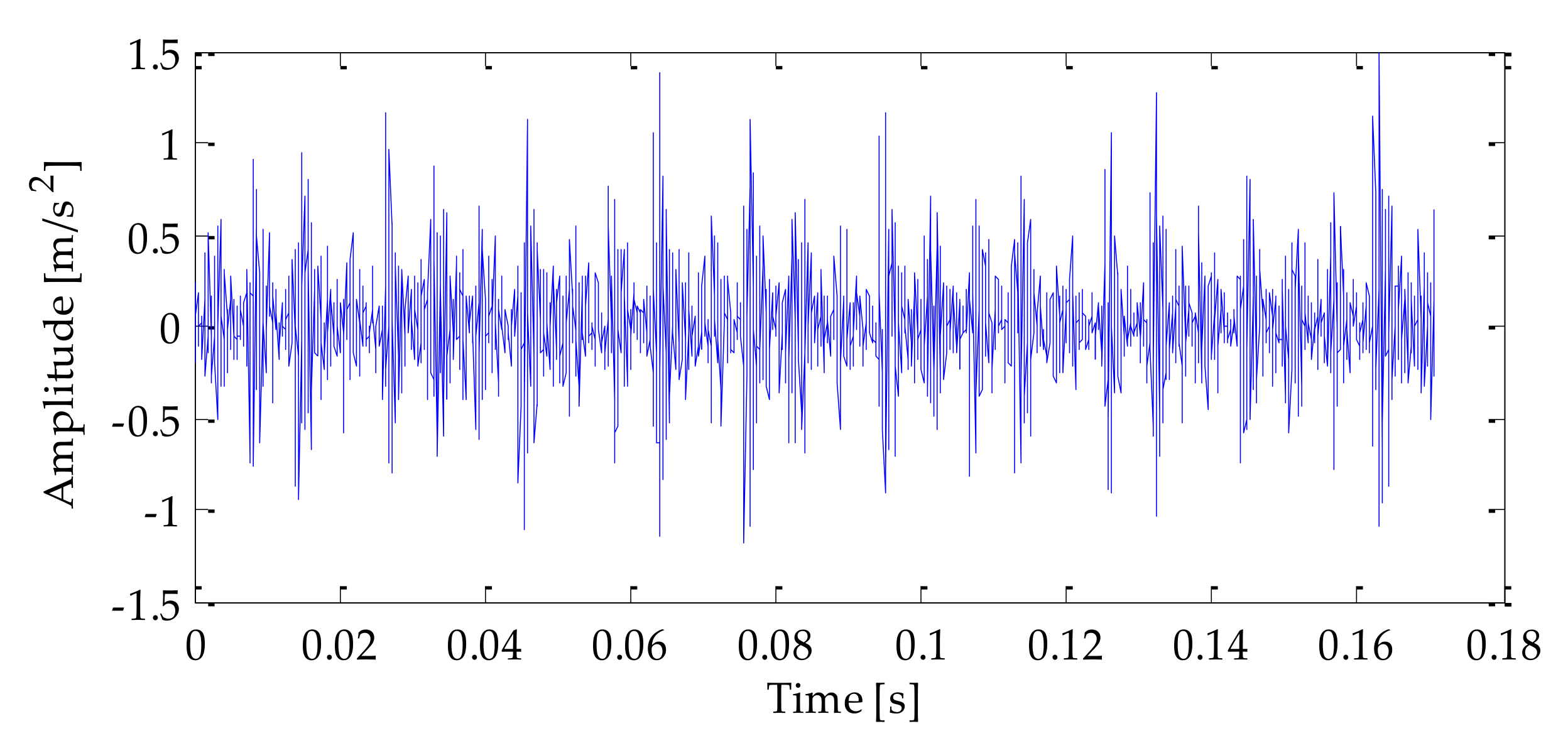
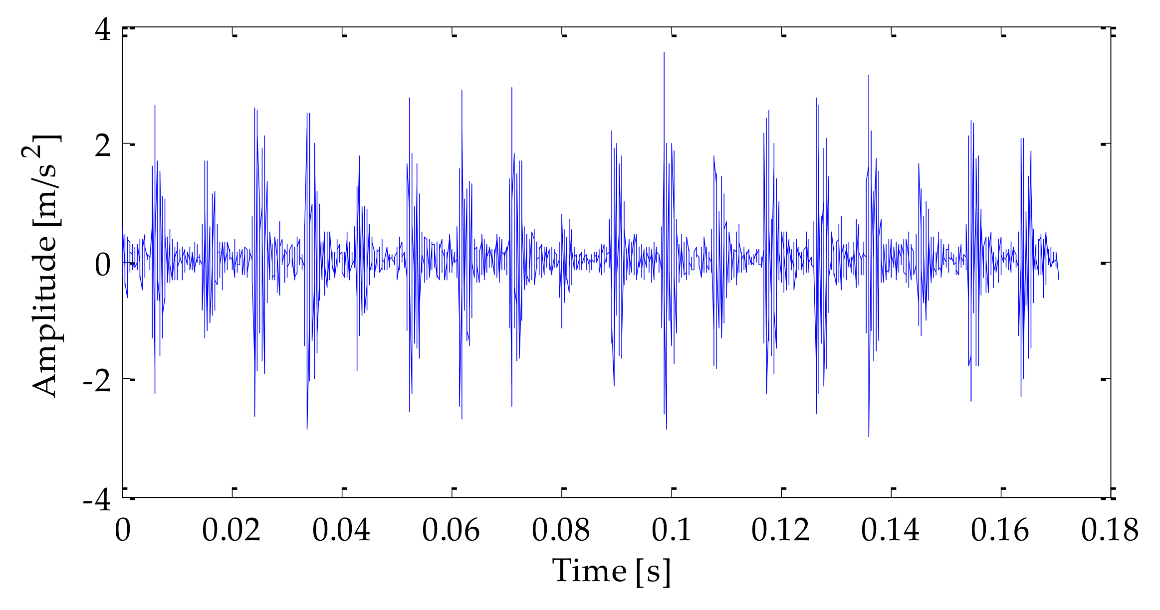
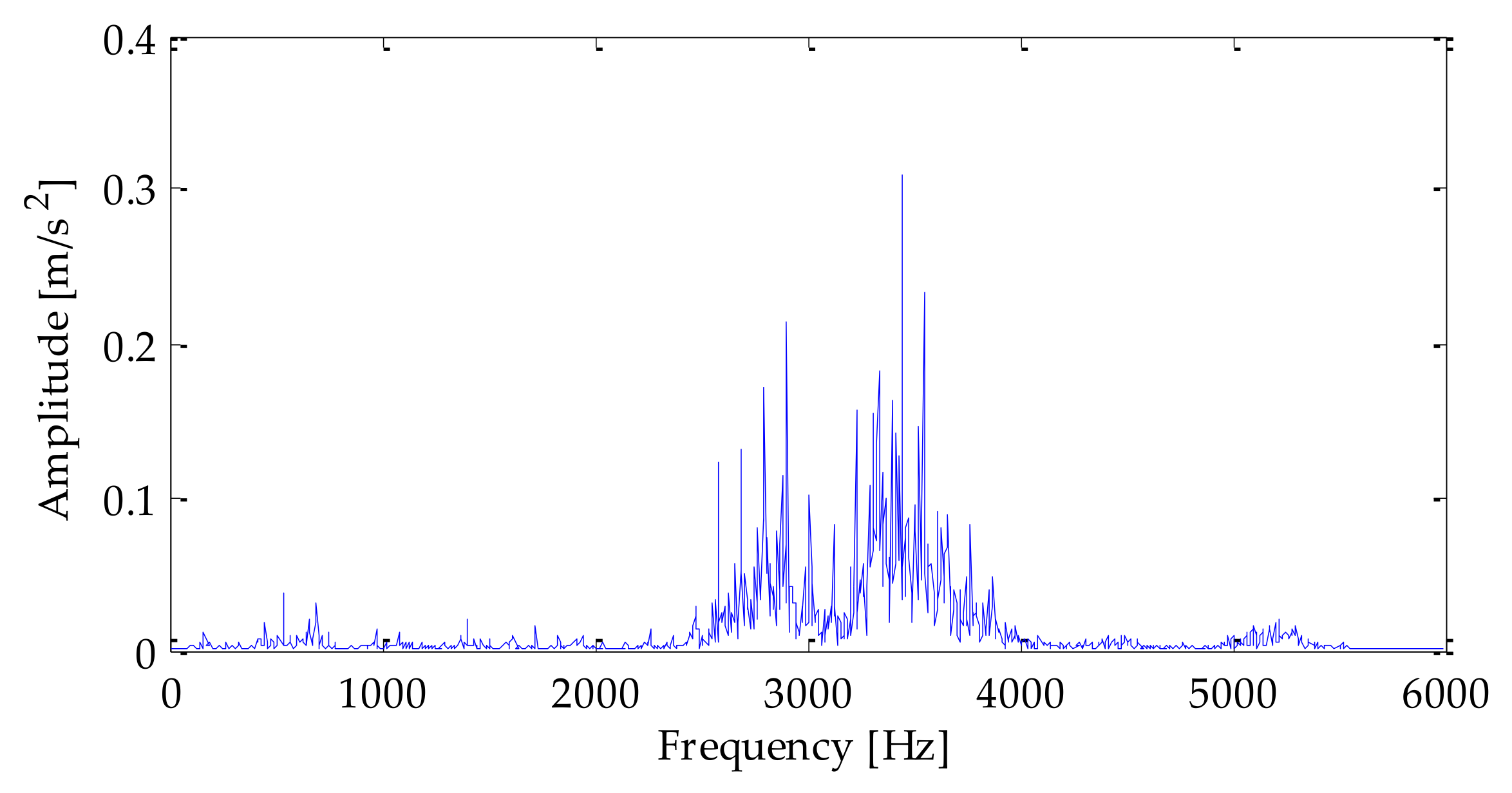
Bearing is one of the most commonly used general parts in all kinds of rotating machinery. It plays a role in bearing and transmitting load in mechanical equipment, and it is very prone to failure. Therefore, to verify the performance of the algorithm proposed in this paper, a typical model was used to simulate the periodic impact signal caused by bearing fault [32]. Firstly, a set of periodic pulse signals was simulated to simulate the fault impact signal, and on this basis, Gaussian white noise was added to the fault impact signal to simulate the bearing fault vibration signal polluted by environmental noise. In this study, Matlab (version R2009a) was selected as the vibration signal modeling and simulation software to build the signal model. The expression of the simulated signal is as follows:

$$s(t)=y_0{e}^{-2\pi f_n\xi t}\mathrm{s}\mathrm{i}\mathrm{n}(2\pi f_n\sqrt{1-{\xi }^2}t)$$

(19)

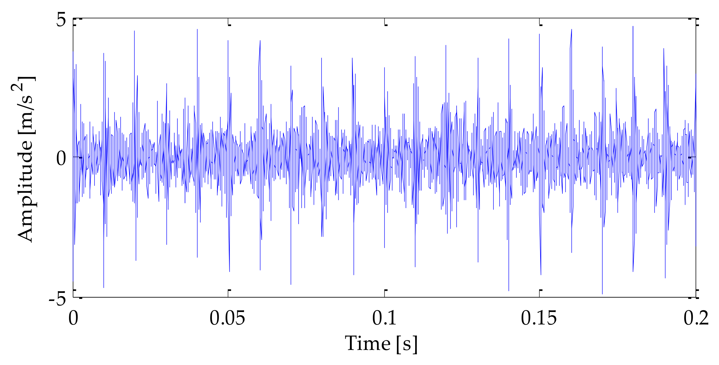
In the above formula: carrier frequency f_n = 3000 Hz, displacement constant y₀ = 5, damping coefficient ξ = 0.1, period T = 0.01 s, sampling frequency f_s = 20 KHz, and number of sampling points n = 4096, where t represents the sampling time. Through calculation, it can be seen that the fault frequency f₀ = 100 Hz. In order to simulate the noise interference of rolling bearing during operation, SNR = −5 dB white Gaussian noise was added to the original signal s(t).

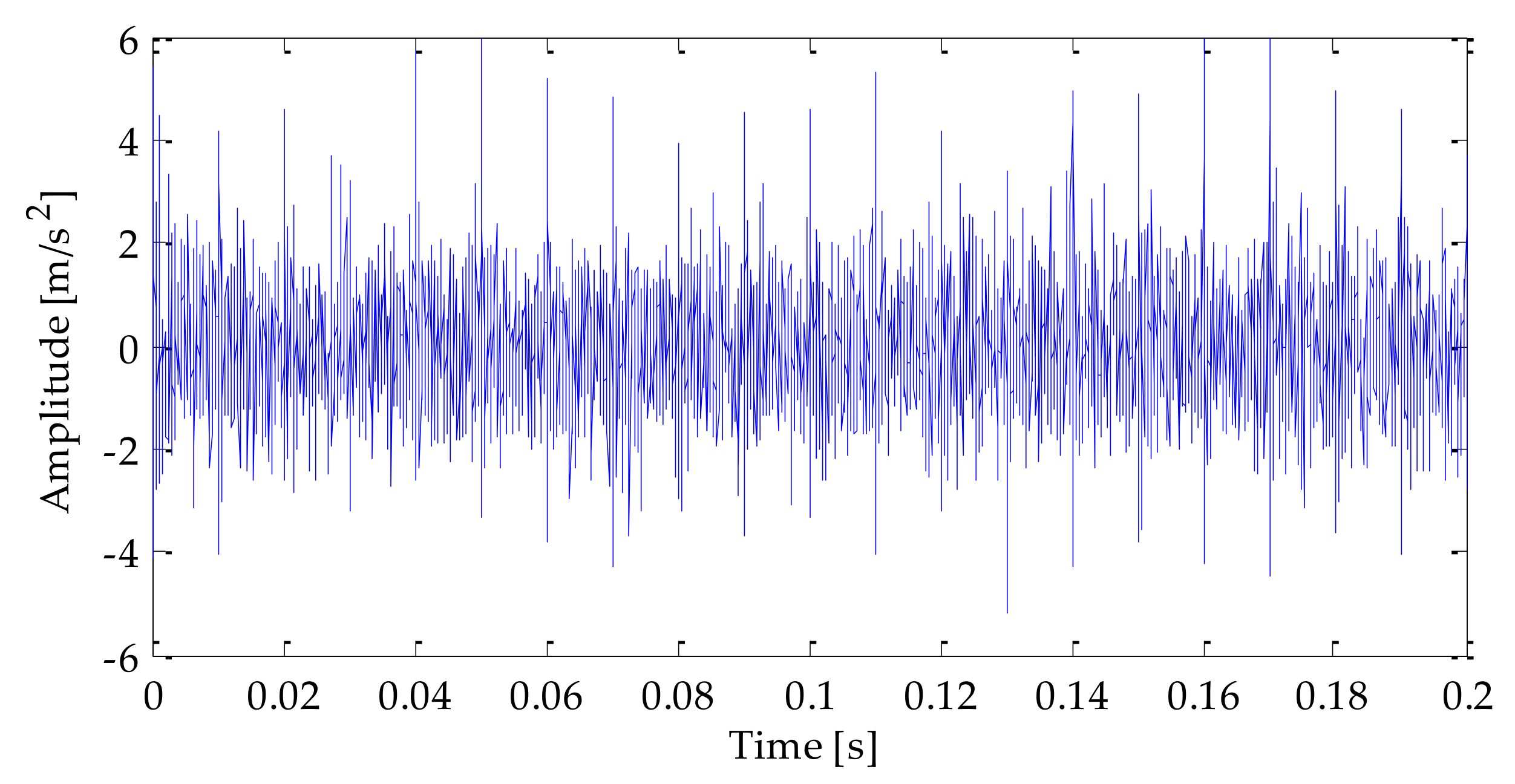
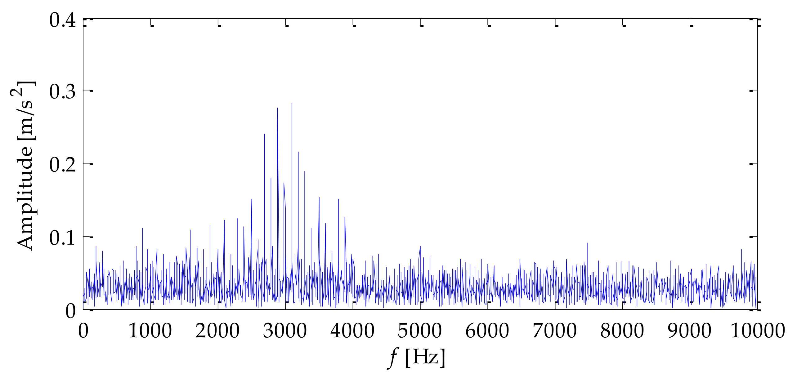
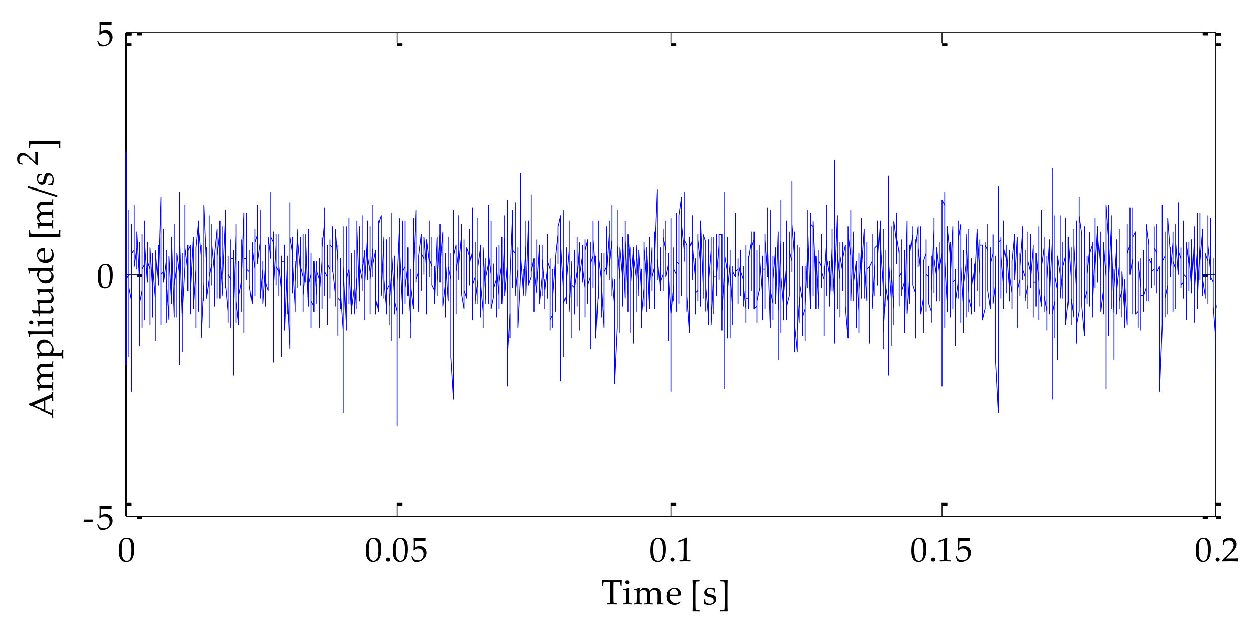
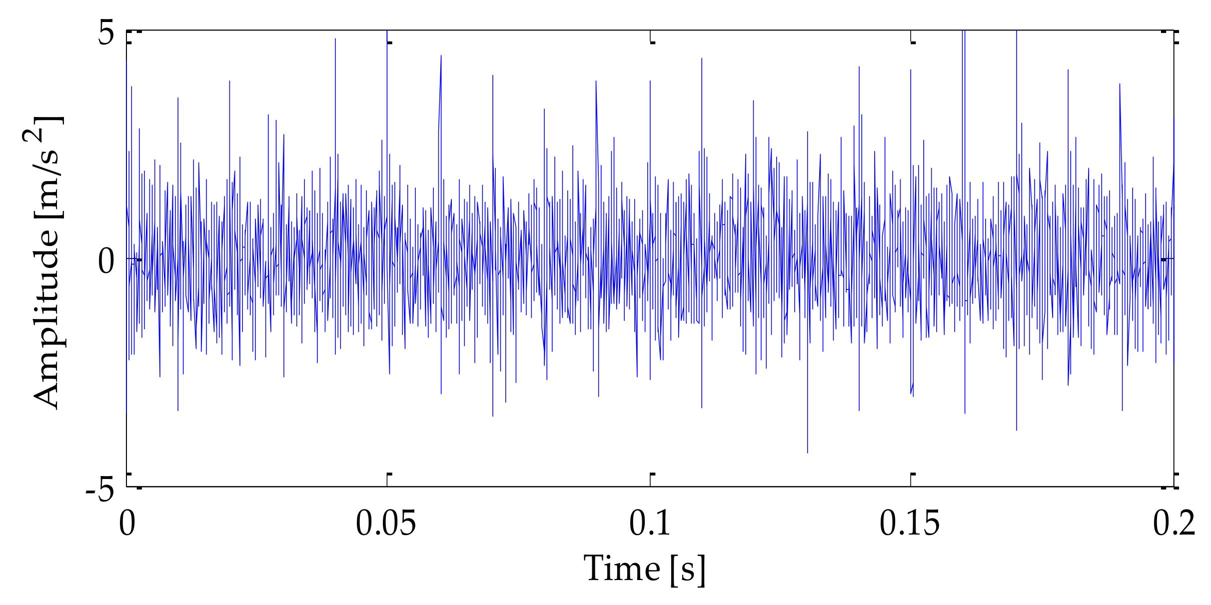
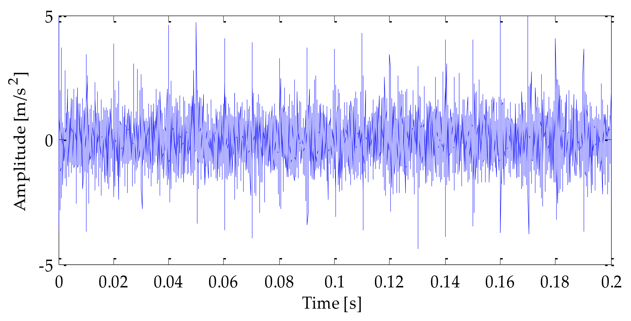
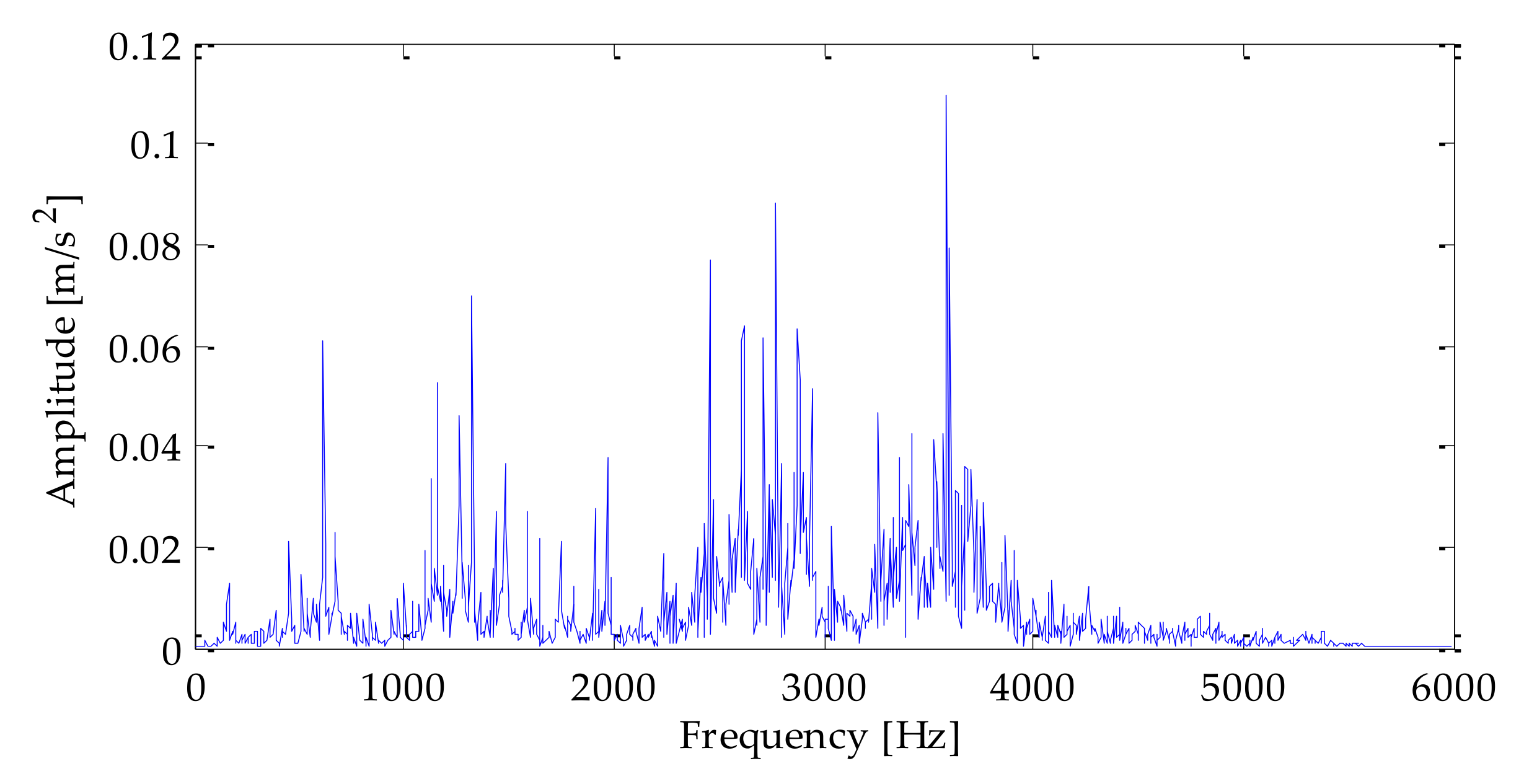
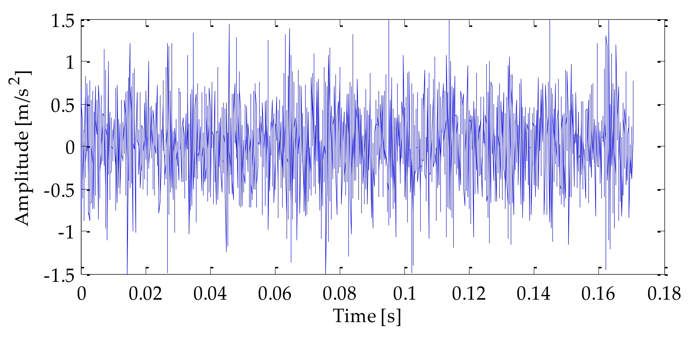
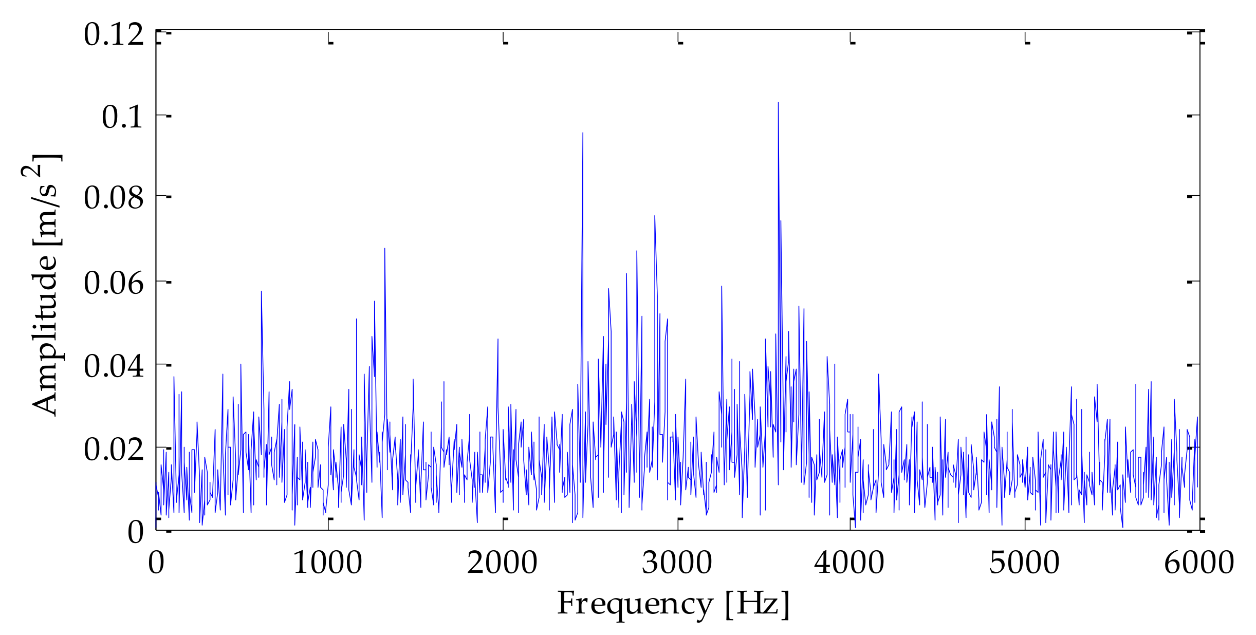
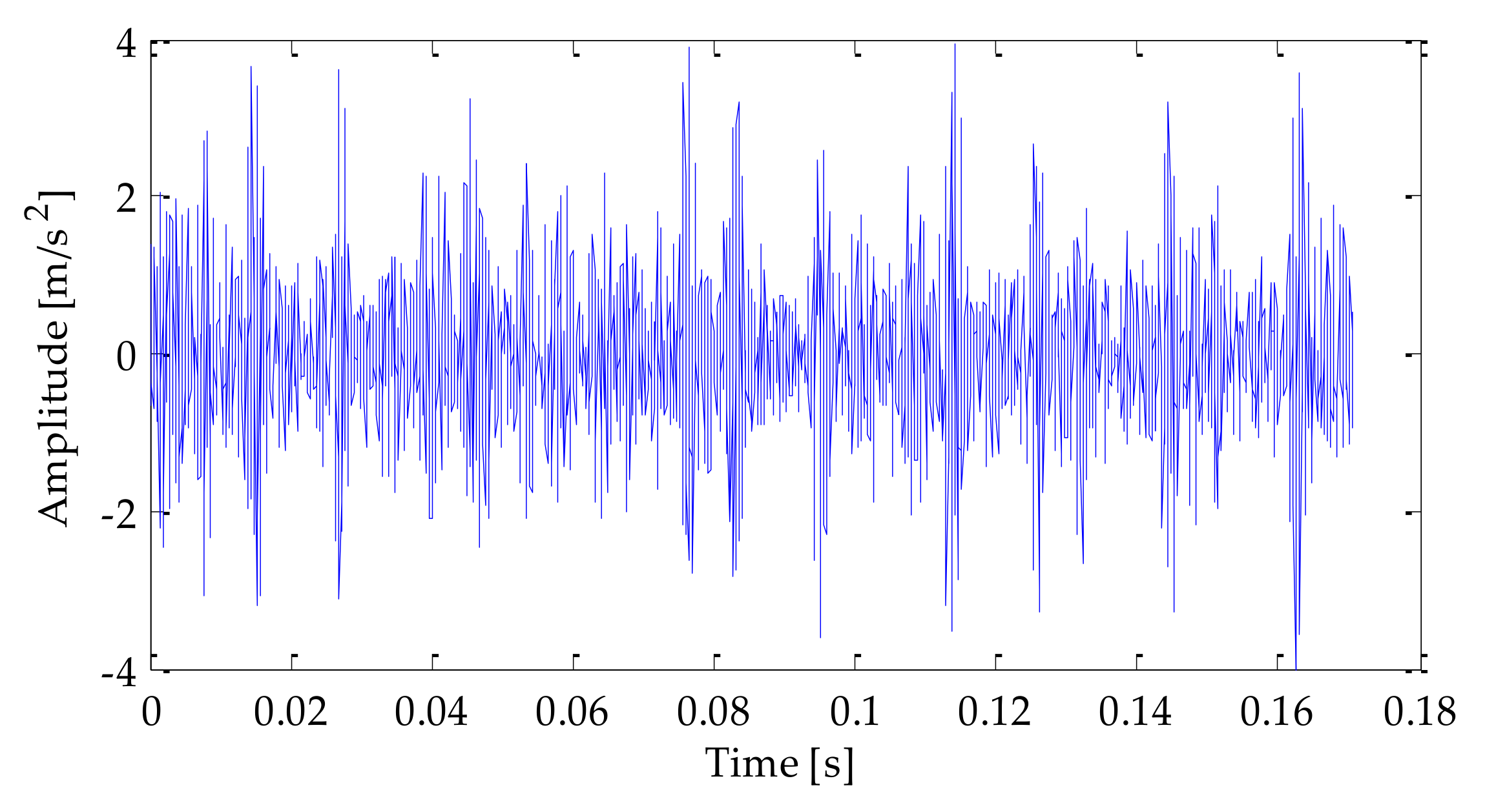
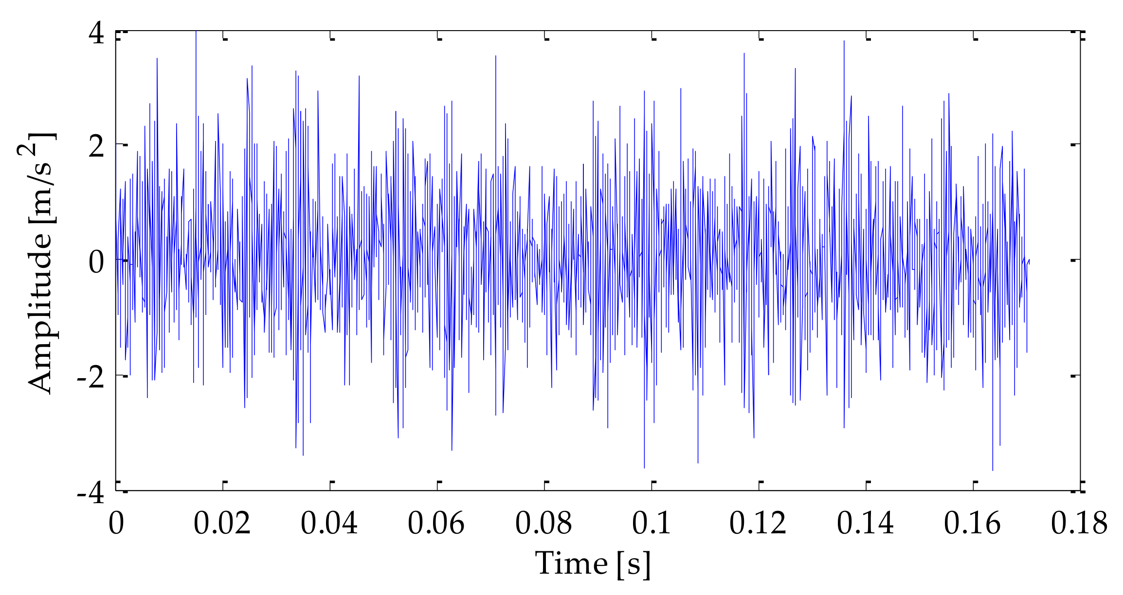
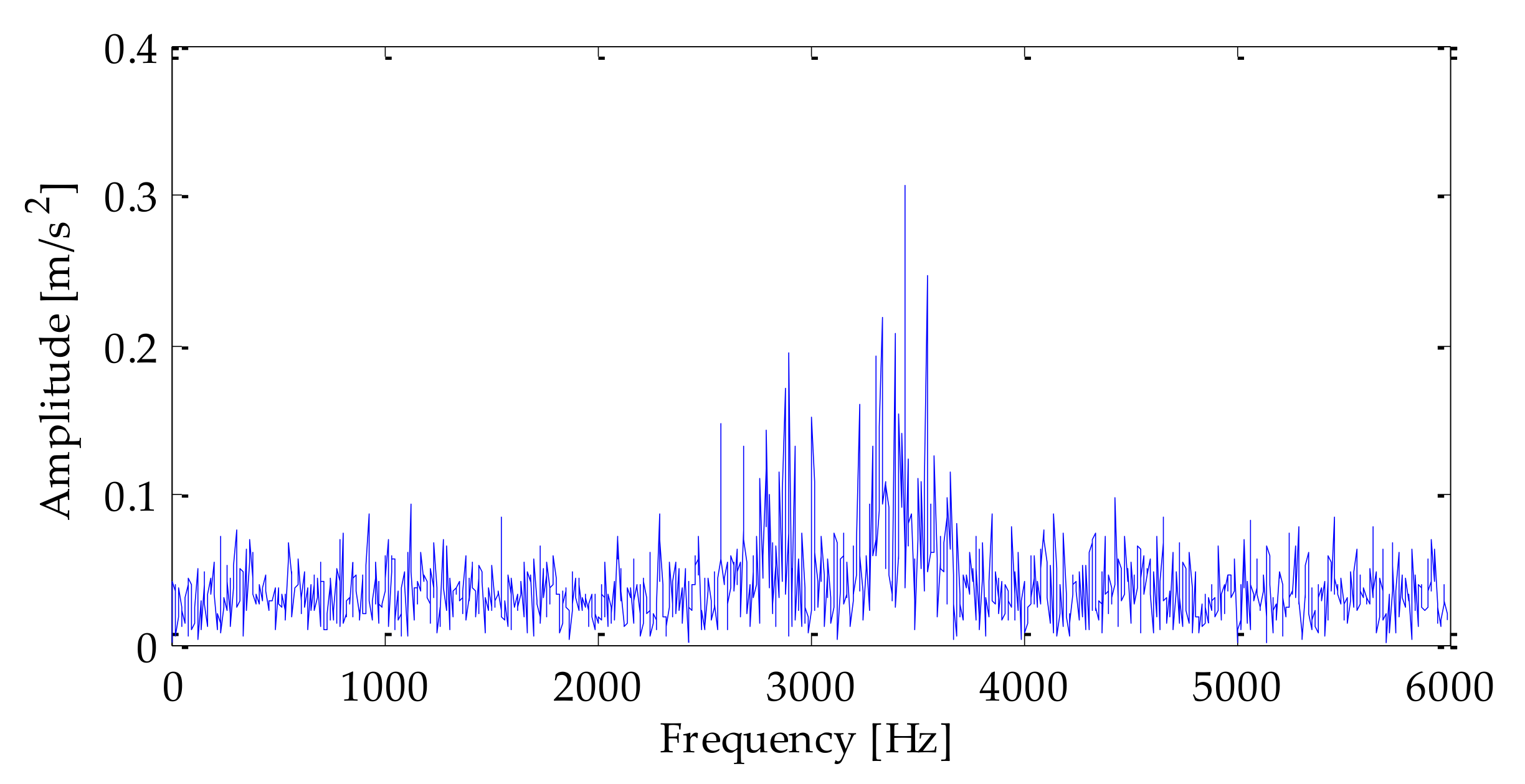
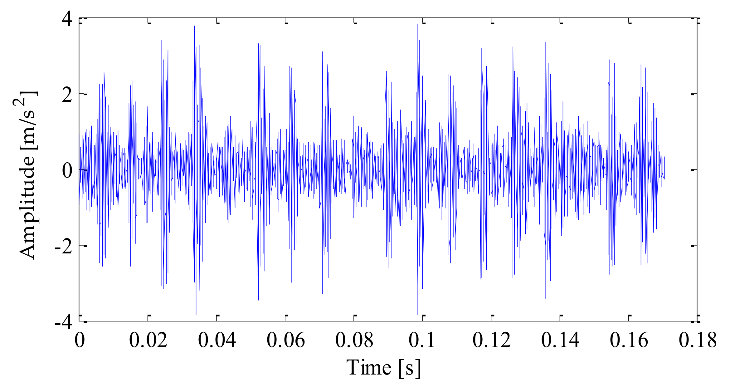
The time–domain waveform of the original signal is shown in Figure 4. After adding noise, the time–domain waveform and frequency–domain waveform of the mixedsignal after adding noise is shown in Figure 5 and Figure 6. Analyzing the above diagrams showsthat most of the impact signal features were covered up under the interference of background noise, which brings some difficulty to the fault feature extraction.

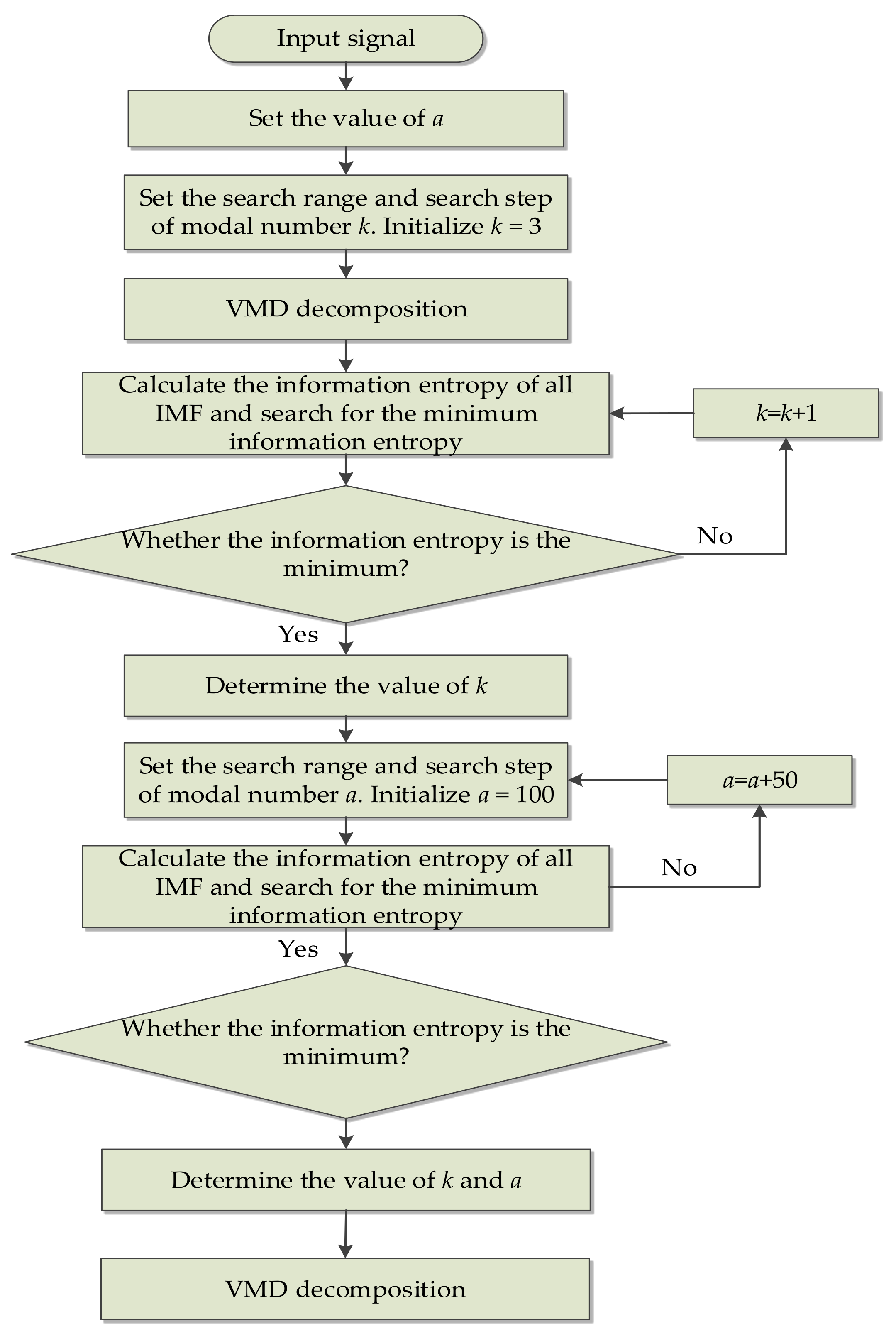
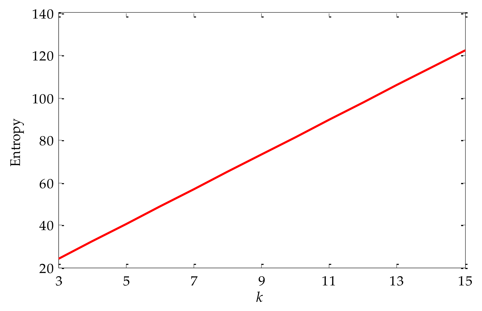
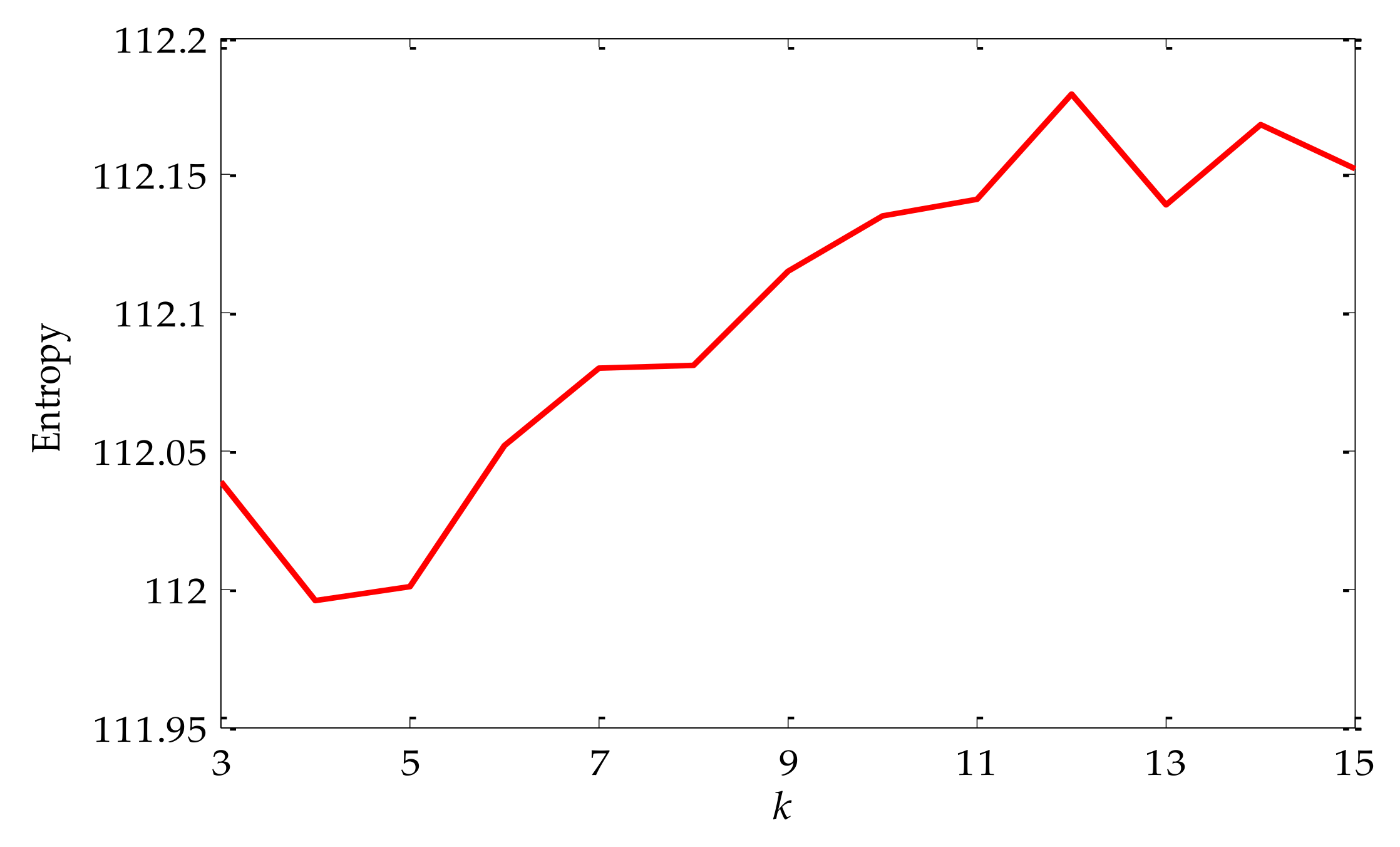
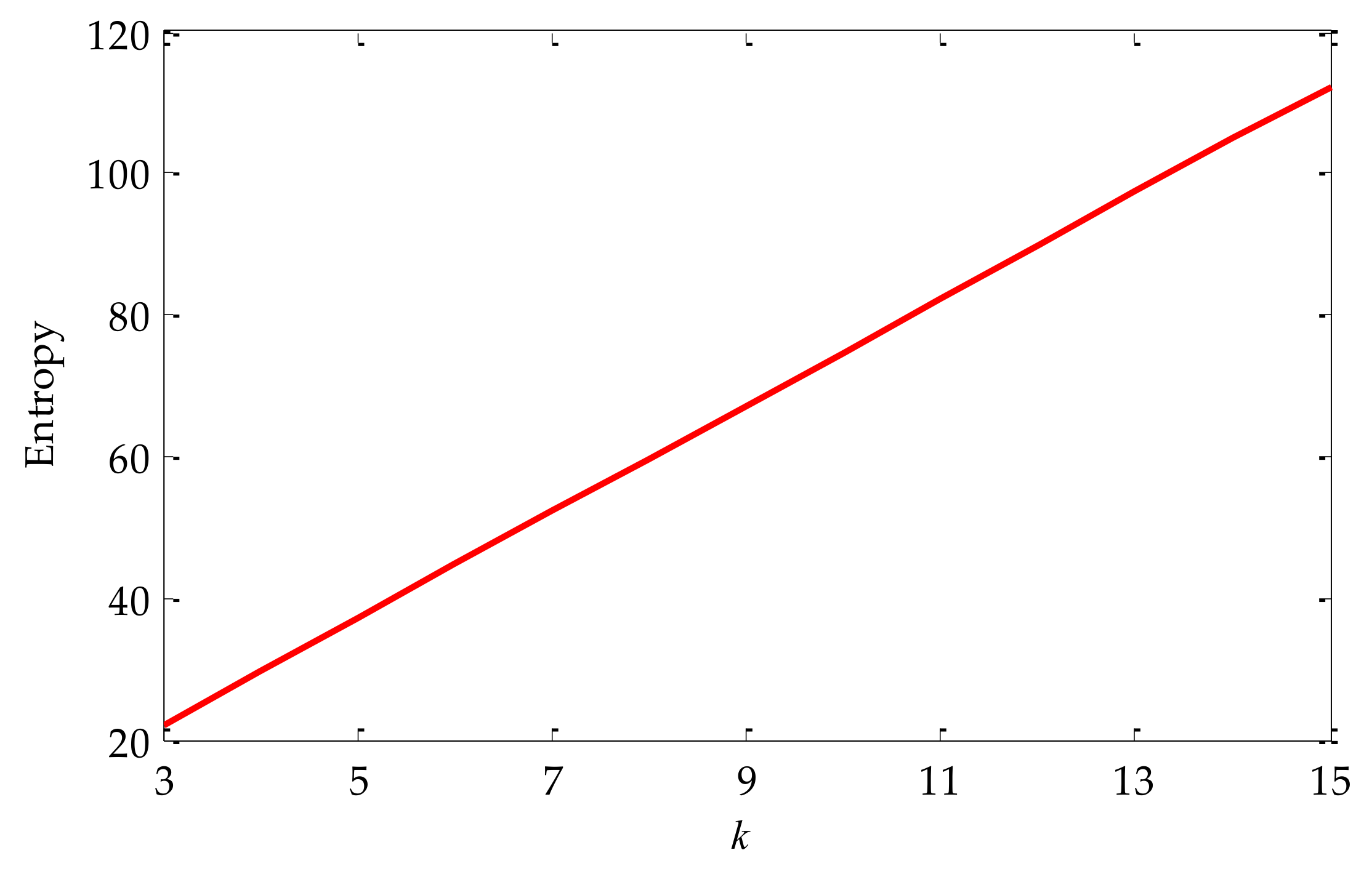
Since the mixed signal was severely interfered with by noise, next, the signal will be decomposed by VMD. Before VMD decomposition, information entropy must be used to optimize VMD to determine the parameters k and α in VMD. Firstly, our experiment used the default value a, which was 2500. Meanwhile, we initialized k = 3, and the search range of k was set to [3,15]. The value of optimal mode k was searched according to the principle of minimum envelope spectral entropy. The relationship between k and envelope spectral entropy is shown in Figure 7. From the transformation trend of the value of k in the figure, it can be seen that with the increasing value of k, the corresponding envelope spectral entropy was also increasing. Therefore, k = 3 was taken as the optimal value.

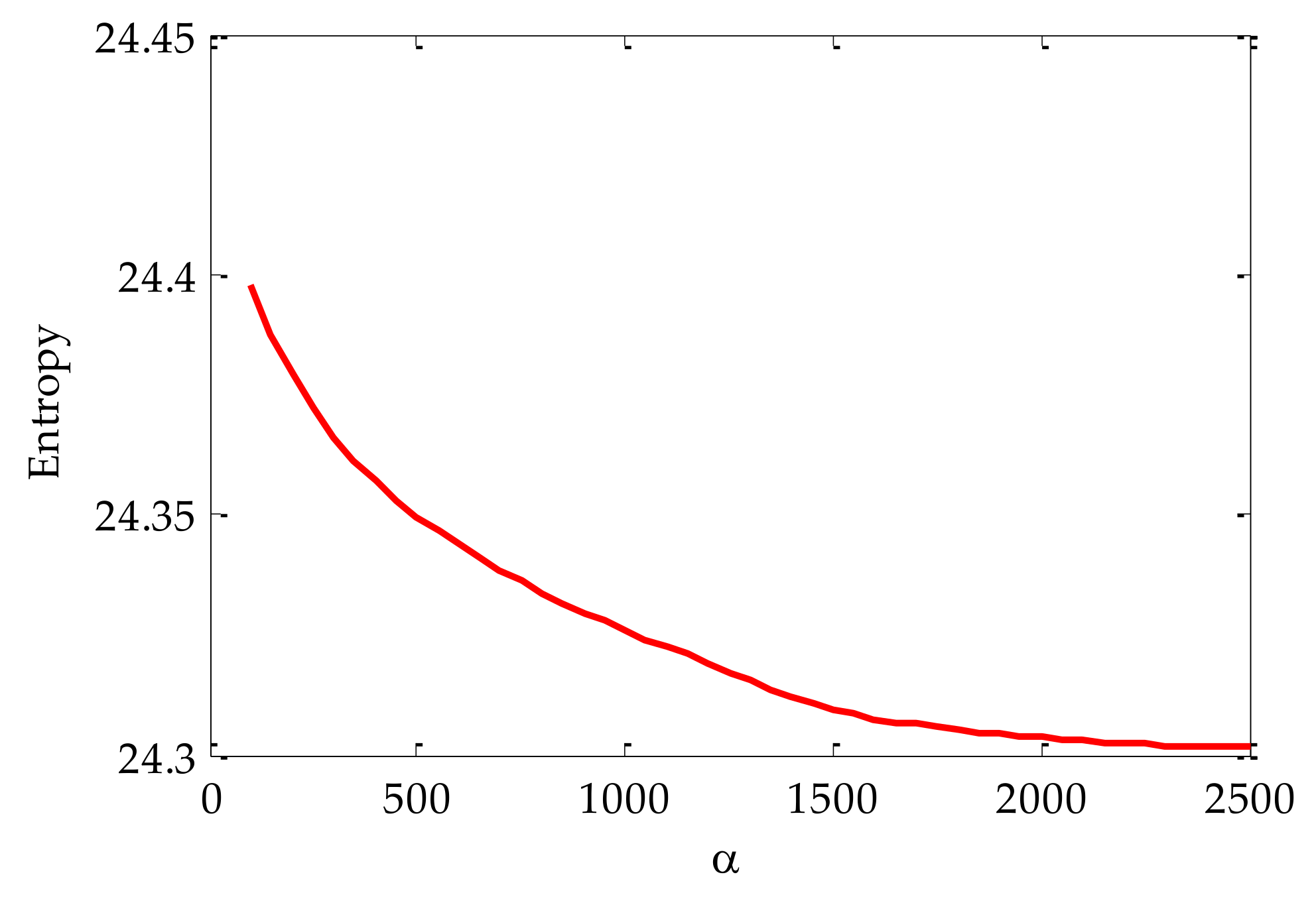
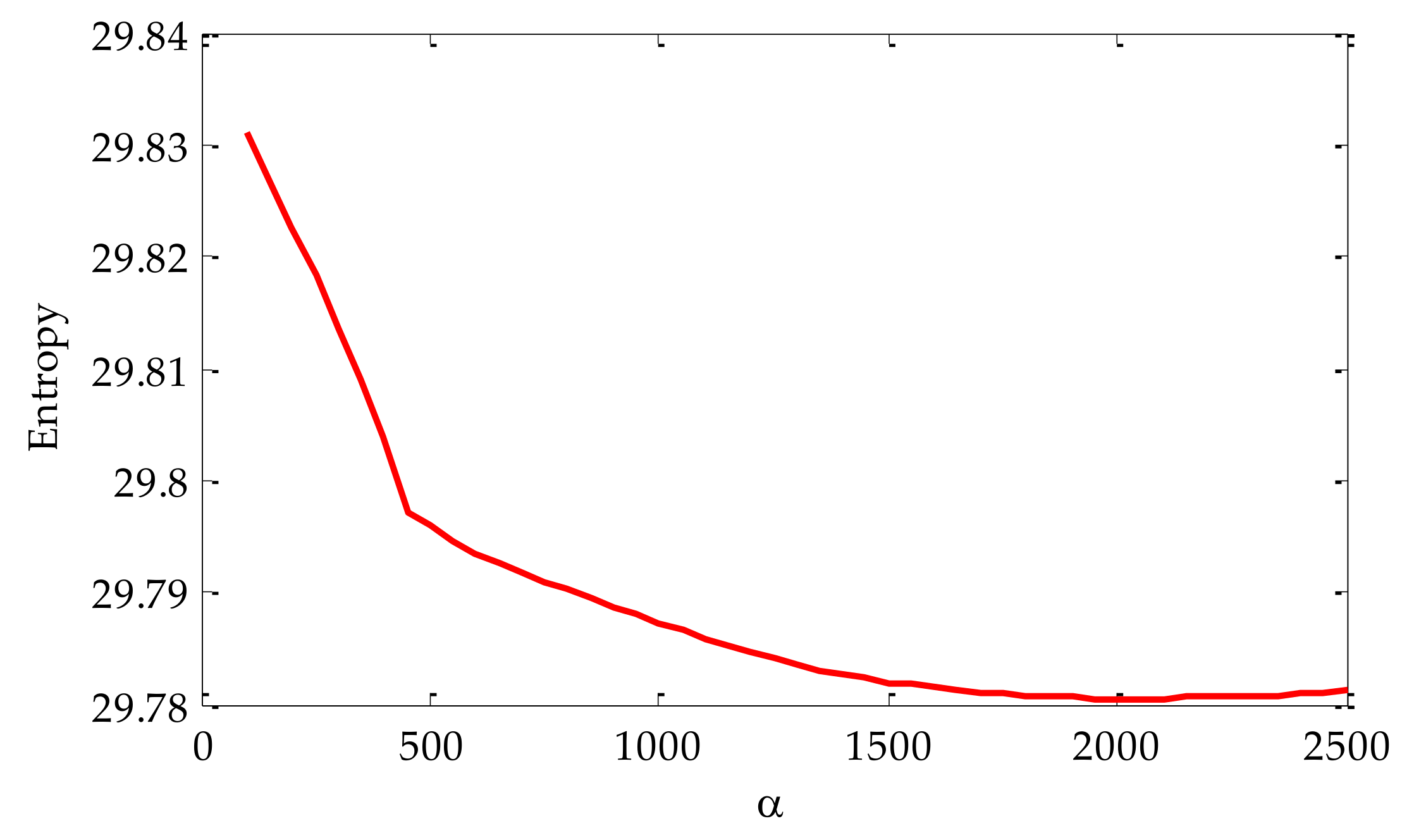
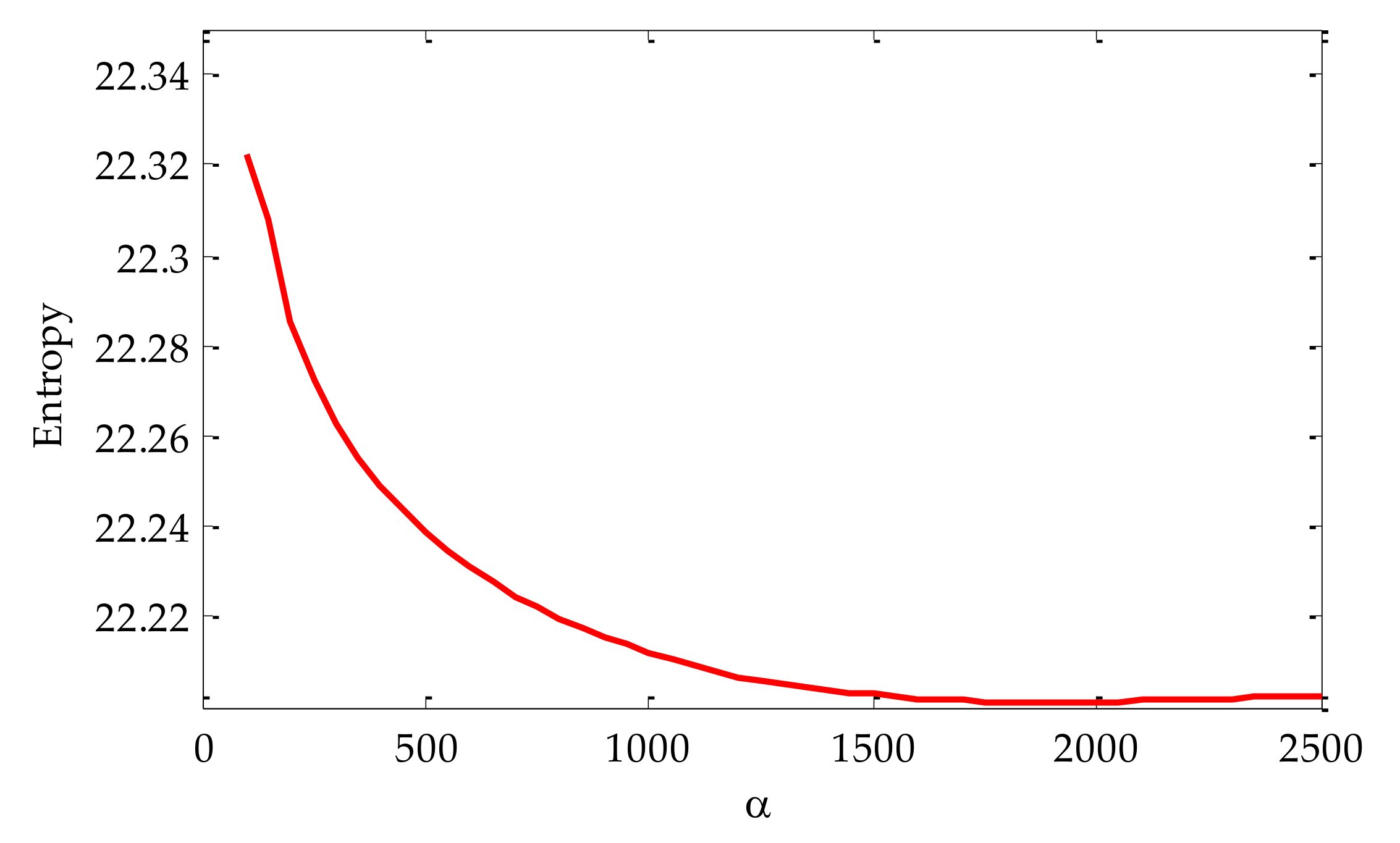
After selecting the value of the optimal mode K, the value of α was then initialized. The search range was set to [100, 2500]. Similarly, the value of the optimal mode α was searched according to the principle of minimum envelope spectral entropy. The relationship with envelope spectral entropy is shown in Figure 8. From the transformation trend of the value of α in the figure, it can be seen that with the continuous increase of α, the value of the corresponding envelope spectral entropy was decreasing and gradually tends to be flat. When the value of α was 2500, the optimal value can be obtained. Therefore, after parameter optimization, the selected optimal parameter combination K and α was [3, 2500].

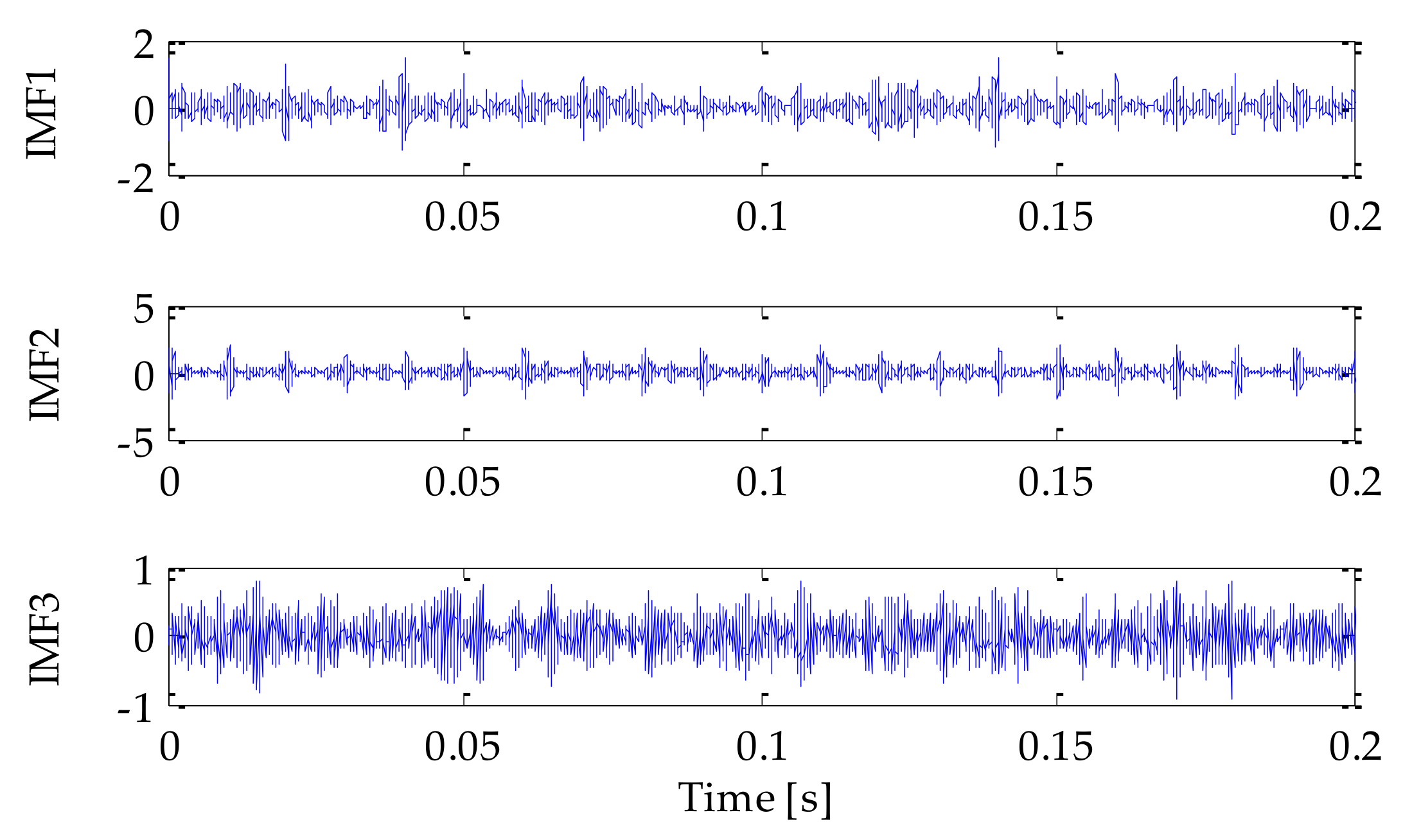
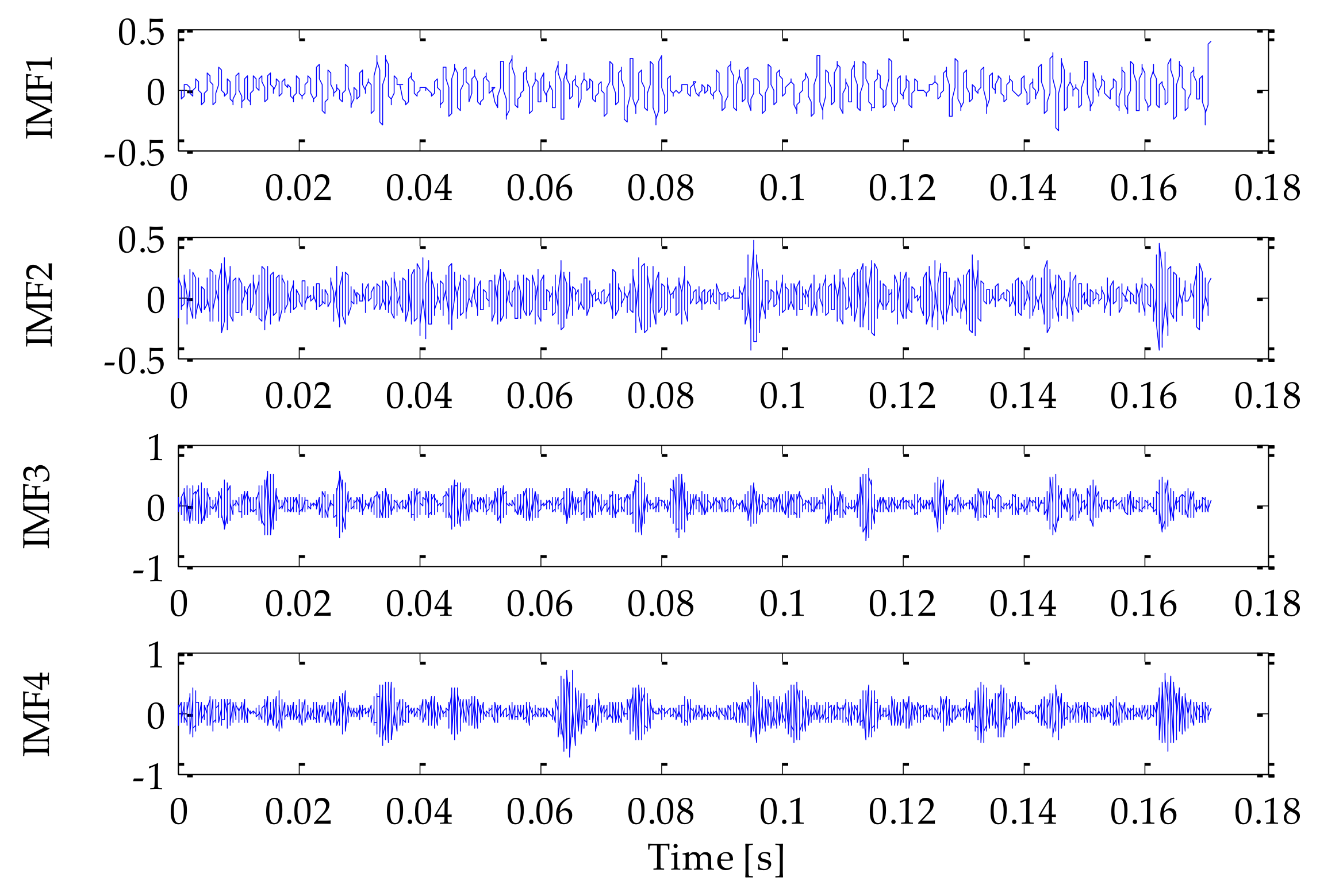
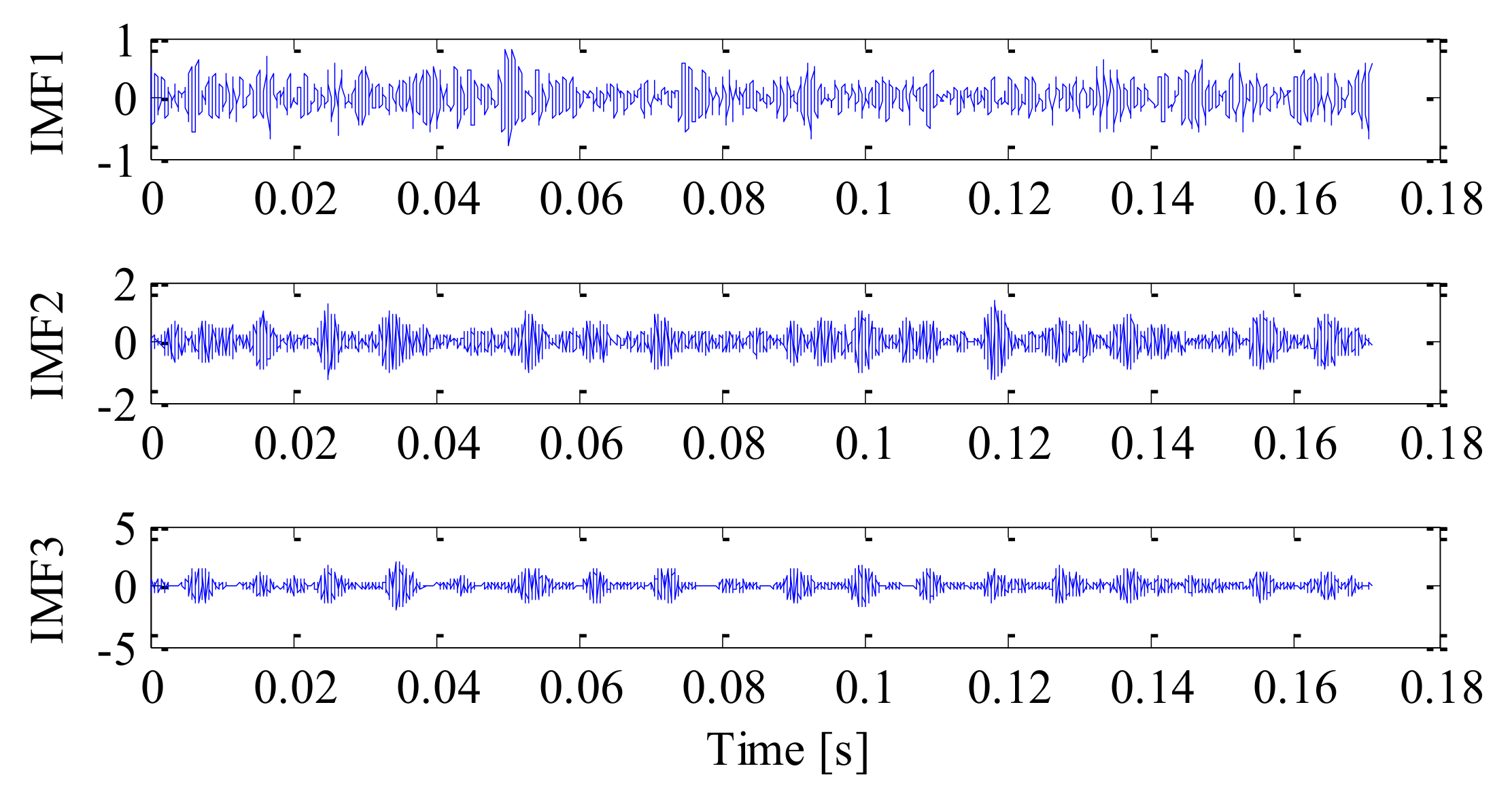
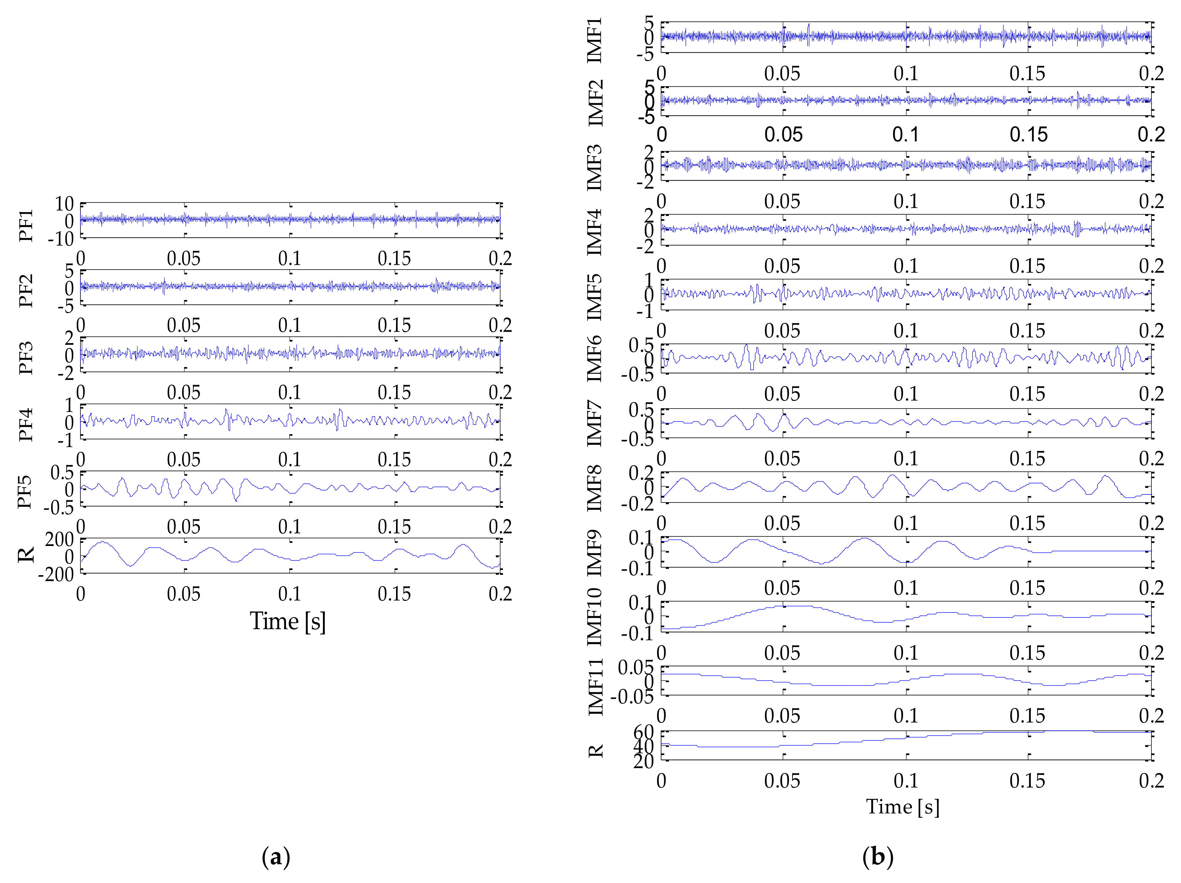
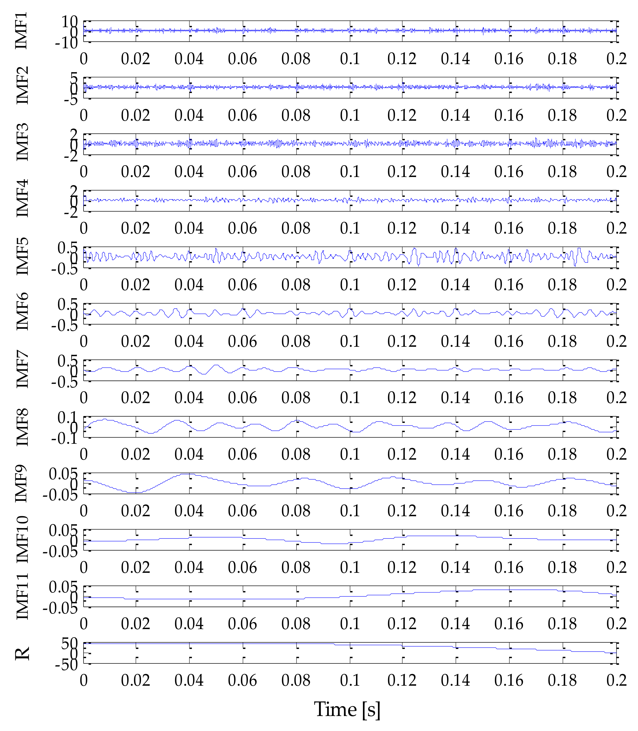
Next, we performed VMD decomposition on the mixed signal. After VMD decomposition optimized by information entropy, three IMF components were obtained. The decomposition results are shown in Figure 9. In order to compare the effects of different methods, the traditional LMD decomposition method, EMD decomposition method, and EEMD decomposition method were used for the time–frequency analysis of mixed signals. The signal decomposition results obtained based on the above three methods are shown in Figure 10a,b. Figure 10 and Figure 11 showed that there were more signal components decomposed by LMD, EMD and EEMD methods, and the signal components obtained by EMD and EEMD had certain modal aliasing and endpoint effect. At the same time, faultycomponents were generated.

To select the appropriate signal component from the decomposition results obtained by the above methods, this experiment will combine kurtosis and cross-correlation coefficient to select. Firstly, all signal components’ correlation coefficient C(t) and kurtosis value Q(t) were calculated. The calculated results are shown in

Table 1. Index values of different IMF signal components (VMD).

Parameter	IMF1	IMF2	IMF3
C(t)	0.433	0.575	0.389
Q(t)	4.402	6.221	2.916

,

Table 2. Index values of different PF signal components (LMD).

Parameter	PF1	PF2	PF3	PF4	PF5
C(t)	0.835	0.418	0.222	0.111	0.062
Q(t)	4.630	4.161	3.572	4.207	3.535

,

Table 3. Index values of different IMF signal components (EMD).

Parameter	IMF1	IMF2	IMF3	IMF4	IMF5	IMF6
C(t)	0.727	0.516	0.283	0.191	0.139	0.107
Q(t)	3.606	4.216	2.833	3.124	2.859	3.116
Parameter	IMF7	IMF8	IMF9	IMF10	IMF11	R
C(t)	0.057	0.038	0.018	0.001	0.009	0.009
Q(t)	4.671	2.318	2.316	3.145	1.505	1.323

and

Table 4. Index values of different IMF signal components (EEMD).

Parameter	IMF1	IMF2	IMF3	IMF4	IMF5	IMF6
C(t)	0.791	0.587	0.353	0.238	0.189	0.127
Q(t)	4.069	3.981	3.248	3.662	3.072	2.818
Parameter	IMF7	IMF8	IMF9	IMF10	IMF11	R
C(t)	0.077	0.045	0.020	0.009	0.013	−0.001
Q(t)	3.503	2.439	2.079	2.239	1.463	2.655

. It can be seen from Table 1 that the IMF1 component and IMF2 component obtained by VMD decomposition meet the conditions that the correlation value was more significant than 0.3 and the kurtosis value was greater than 3. This shows that the correlation between the above two signal components and the original signal was high, and the signal contained more impact components. Therefore, the IMF1 and IMF2 components were selected to reconstruct the observation signal channel. Secondly, it can be seen from Table 2 that the PF1 component and PF2 component obtained by LMD decomposition met the conditions that the correlation value is more significantthan 0.3 and the kurtosis value is greater than 3. Therefore, PF1 component and PF2 component were selected to reconstruct the observation signal channel. Meanwhile, it can be seen from Table 3 that the IMF1 component and IMF2 component obtained by EMD decomposition met the conditions that the correlation value is more significantthan 0.3 and the kurtosis value is greater than 3. Therefore, IMF1 and IMF2 components were selected to reconstruct the observation signal channel. It can be seen from Table 4 that the IMF1 component, IMF2 component and IMF3 component obtained by EEMD decomposition meet the conditions that the correlation value is more significant than 0.3 and the kurtosis value is greater than 3. Therefore, the above three signal components were selected to reconstruct the observation signal channel, and the remaining signal components were used to reconstruct the noise signal channel. Finally, on this basis, the RobustICA algorithm was used to separate signal and noise. The noise-reduction results obtained by using the method proposed in this paper and LMD–RobustICA, EMD–RobustICA, and EEMD–RobustICA are shown in Figure 12,Figure 13, Figure 14 and Figure 15.

By analyzing the noise-reduction results in Figure 12, Figure 13, Figure 14 and Figure 15, it can be seen that after the noise-reduction method proposed in this article, the impact components in the signal have been revealed. In contrast, the results obtained by the LMD–RobustICA, EMD–RobustICA, and EEMD–RobustICA were not significant. To further analyze the effect of noise reduction, the experiment selected four indicators of kurtosis value, cross-correlation coefficient, root mean square error (RMSE), and mean absolute error (MAE) as evaluation indicators. After calculation, the results obtained are shown in

Table 5. Comparison of noise-reduction effect index values.

Evaluation Index	LMD–RobustICA	EMD–RobustICA	EEMD–RobustICA	Proposed Method
Kurtosis	4.231	4.609	4.614	6.162
correlation coefficient	0.462	0.505	0.518	0.681
RMSE	1.009	0.867	0.858	0.740
MAE	0.611	0.691	0.690	0.583

. In Table 5, by using the method proposed in this paper, the correlation value and kurtosis value obtained after noise reduction were the largest, while the RMSE and the MAE were the smallest. However, the four groups of evaluation index values obtained after noise reduction using LMD–RobustICA, EMD–RobustICA, and EEMD–RobustICA were relatively poor. Therefore, after quantitative analysis, it can be known that the signal obtained after noise reduction using the method proposed in this paper contained a higher impact component, a greater degree of correlation with the original signal, and a relatively higher waveform similarity.

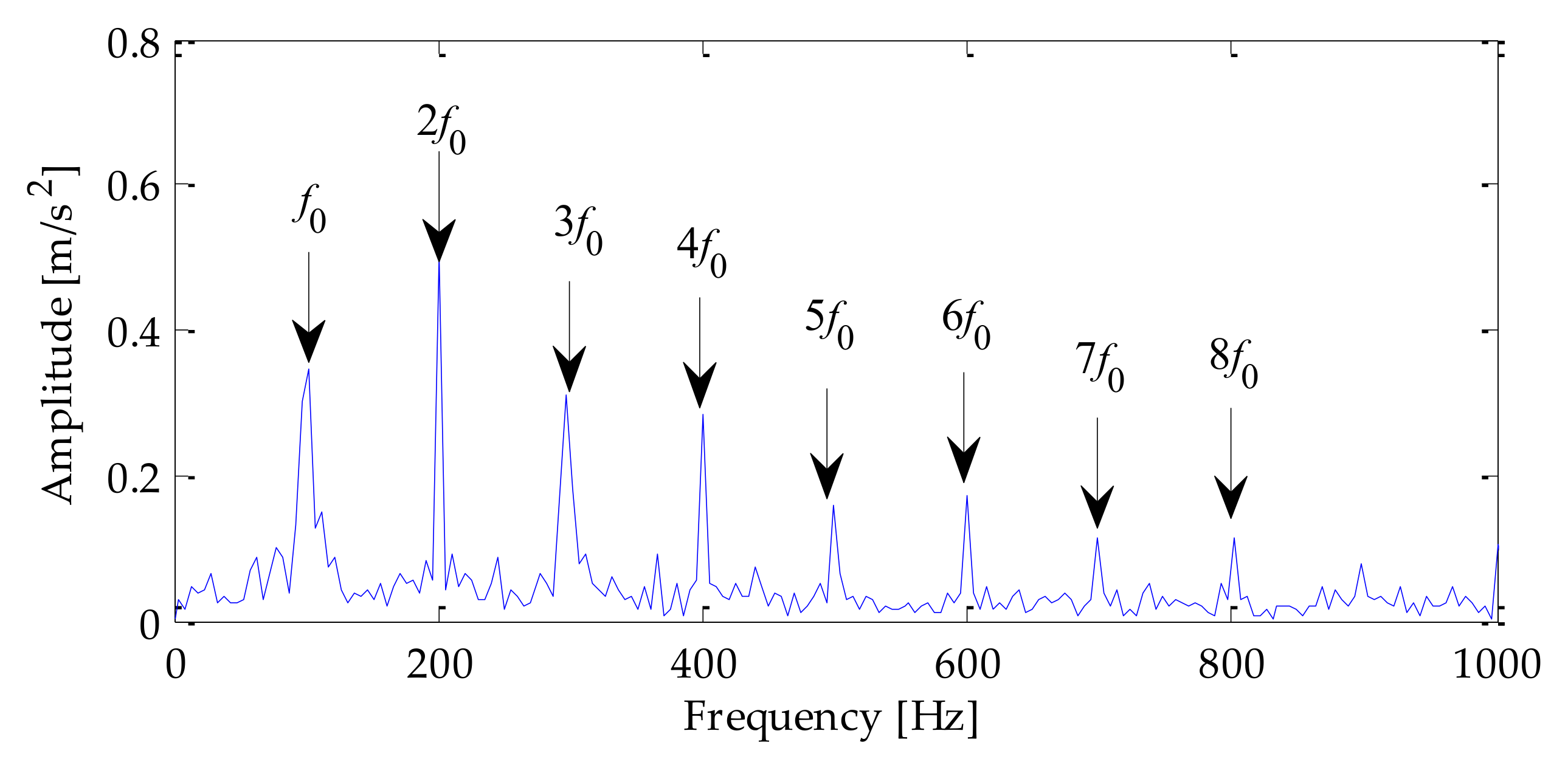
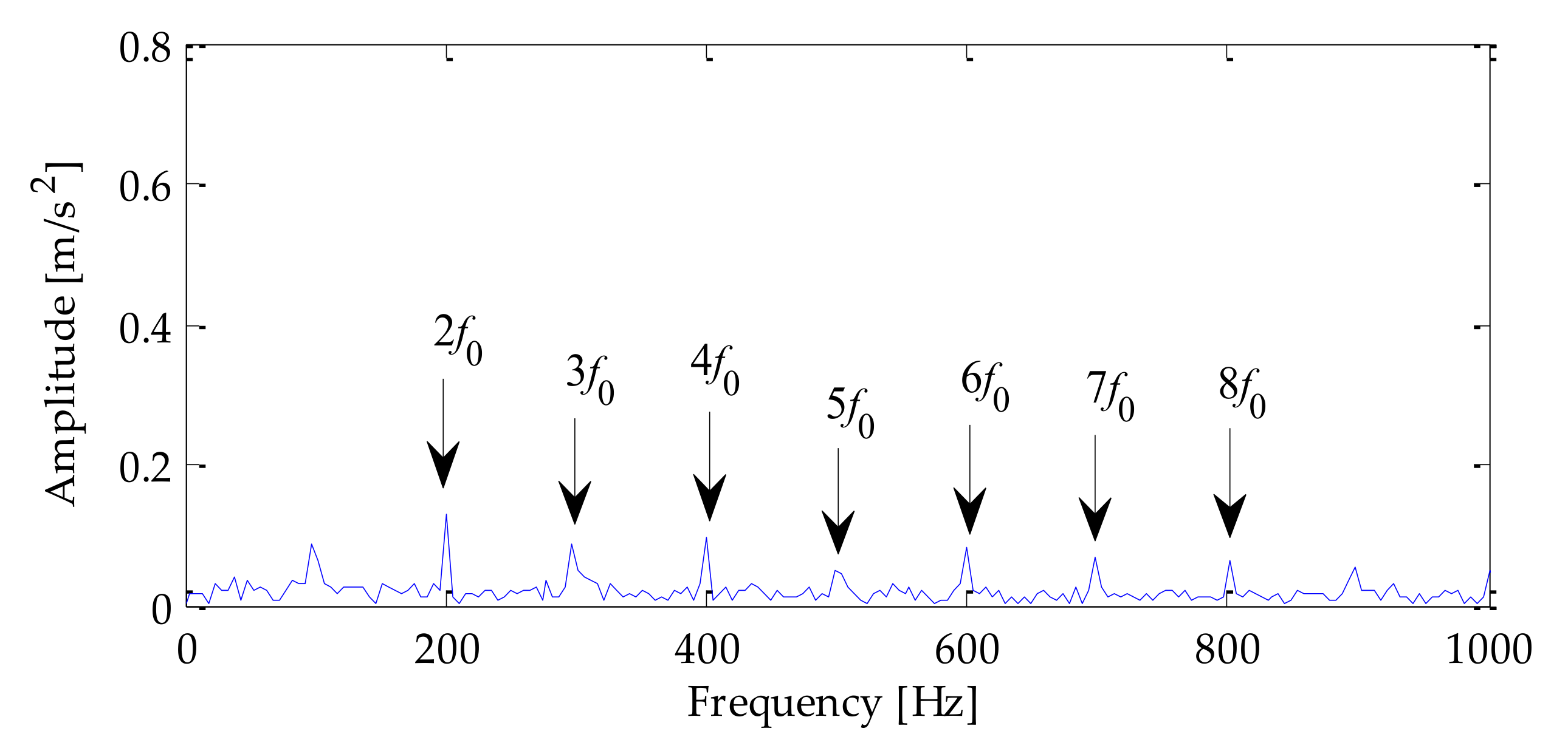
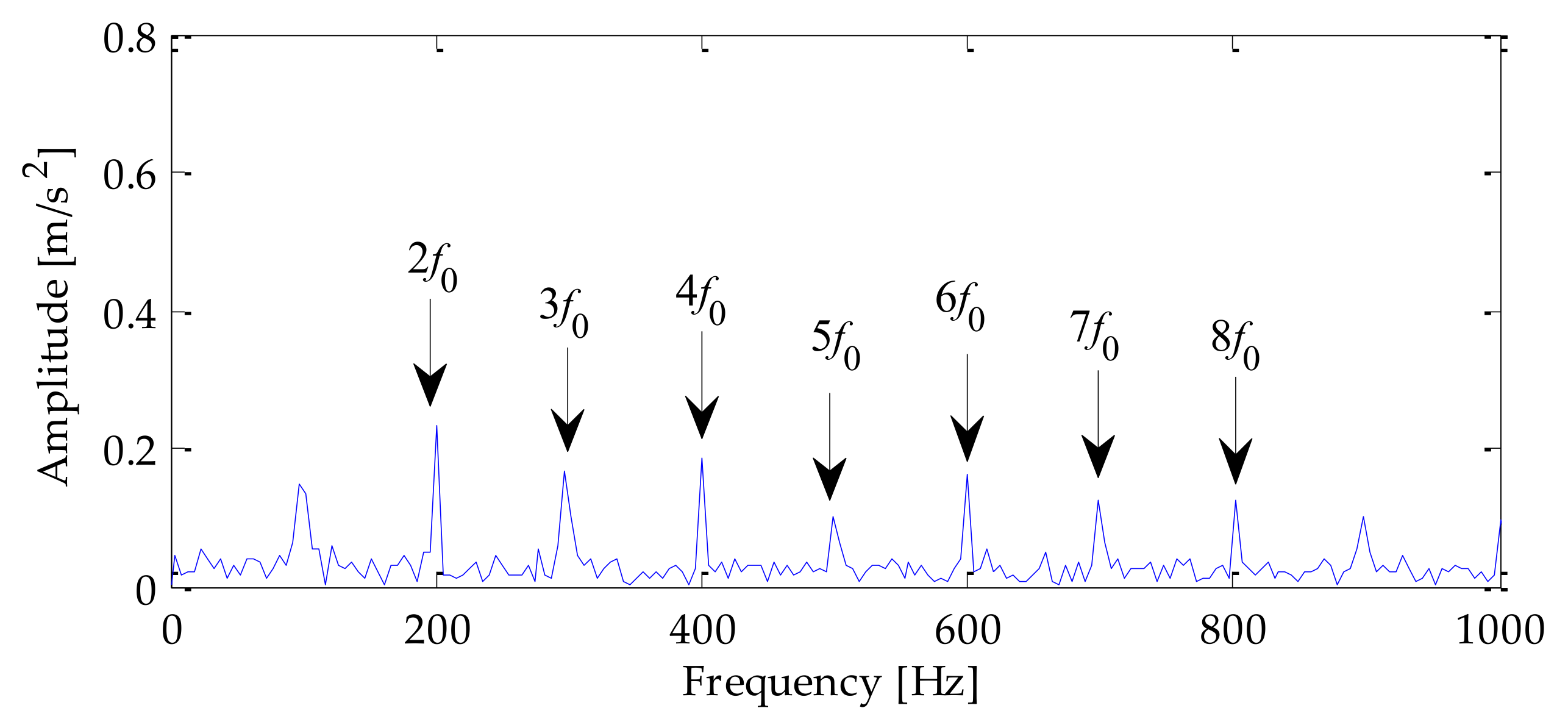
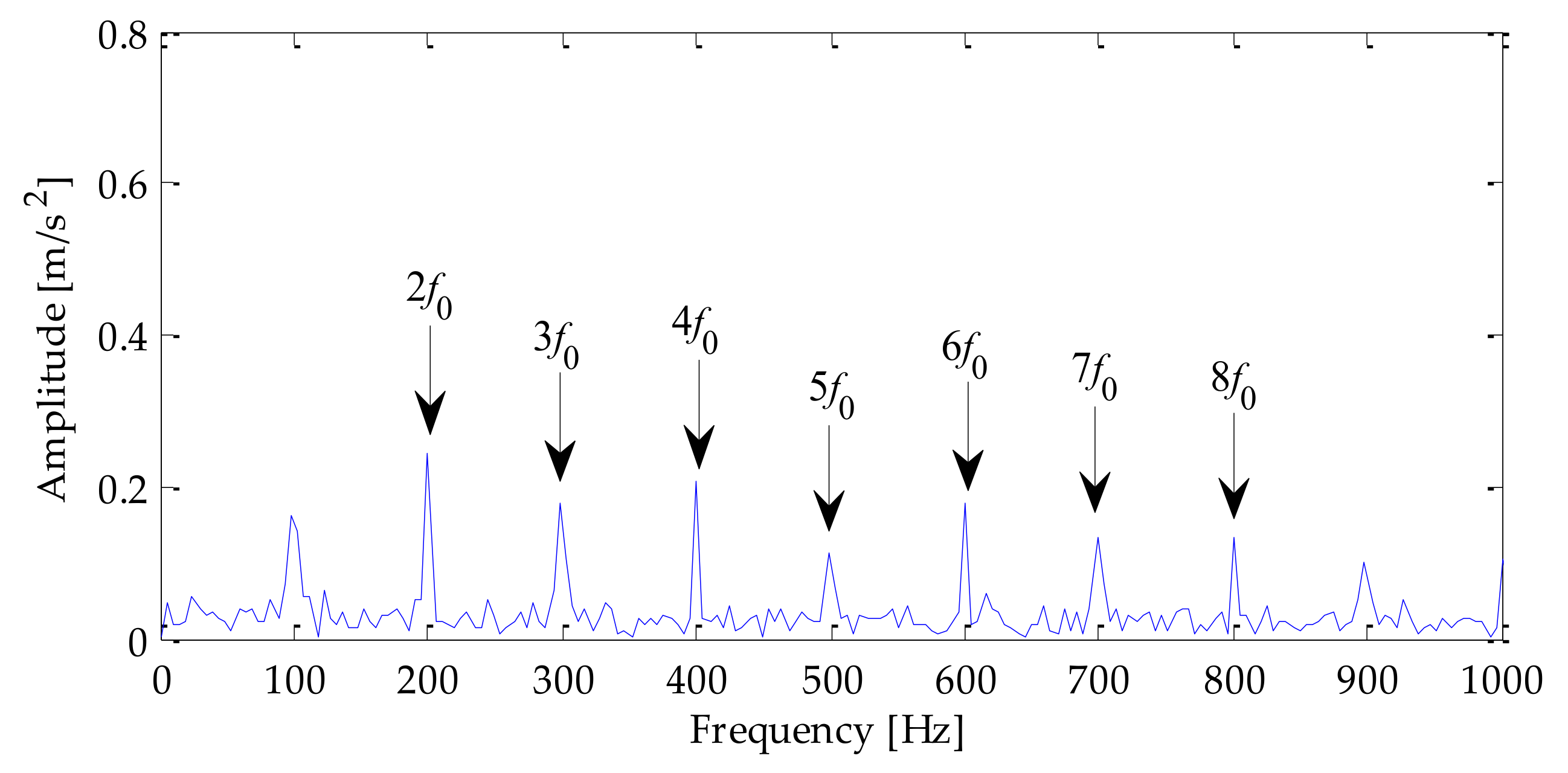
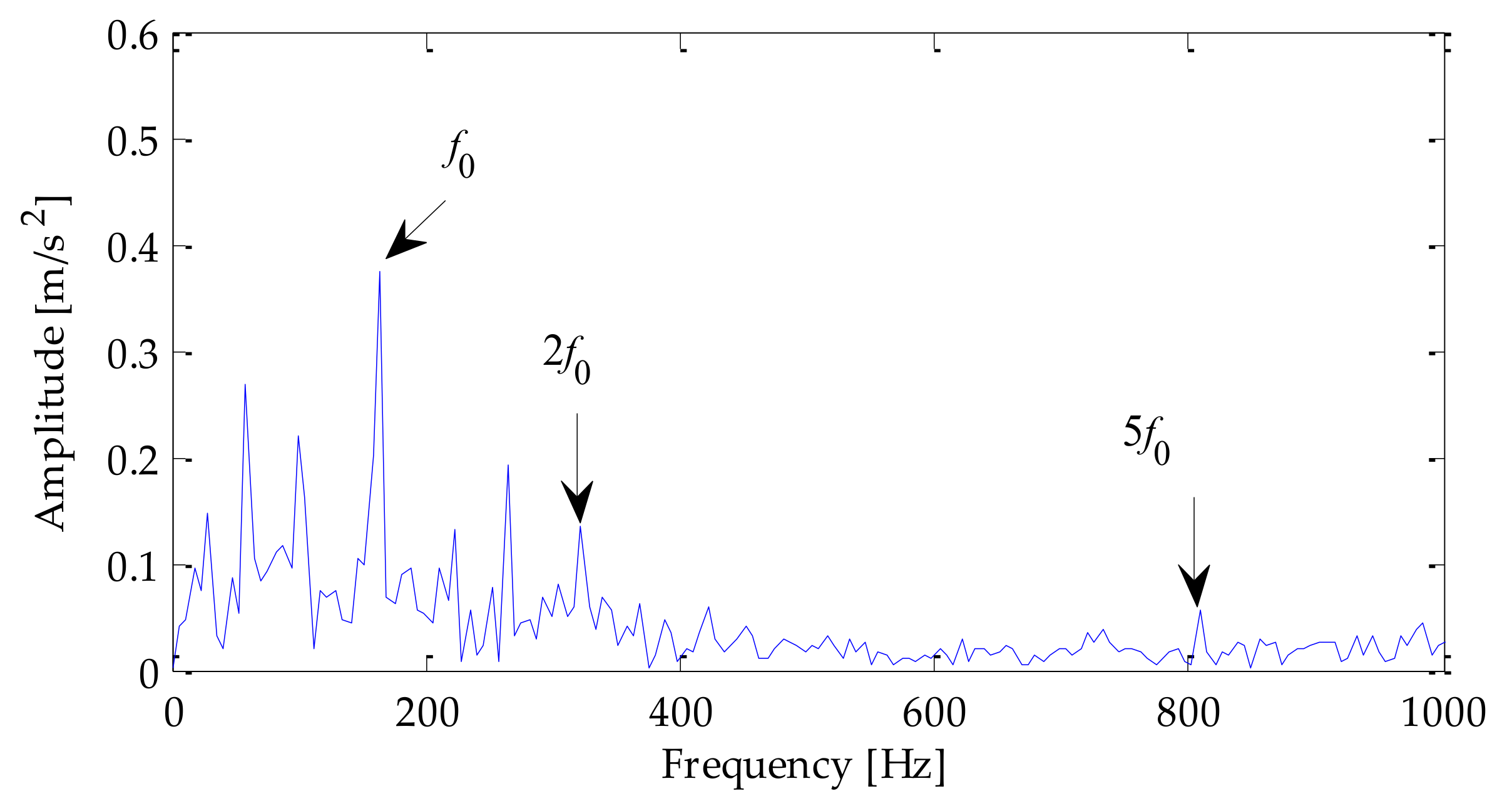
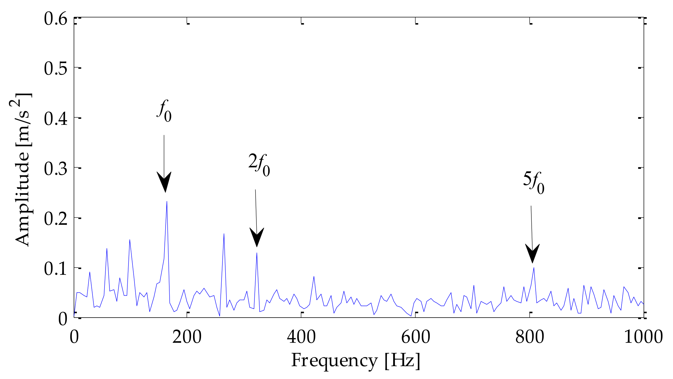
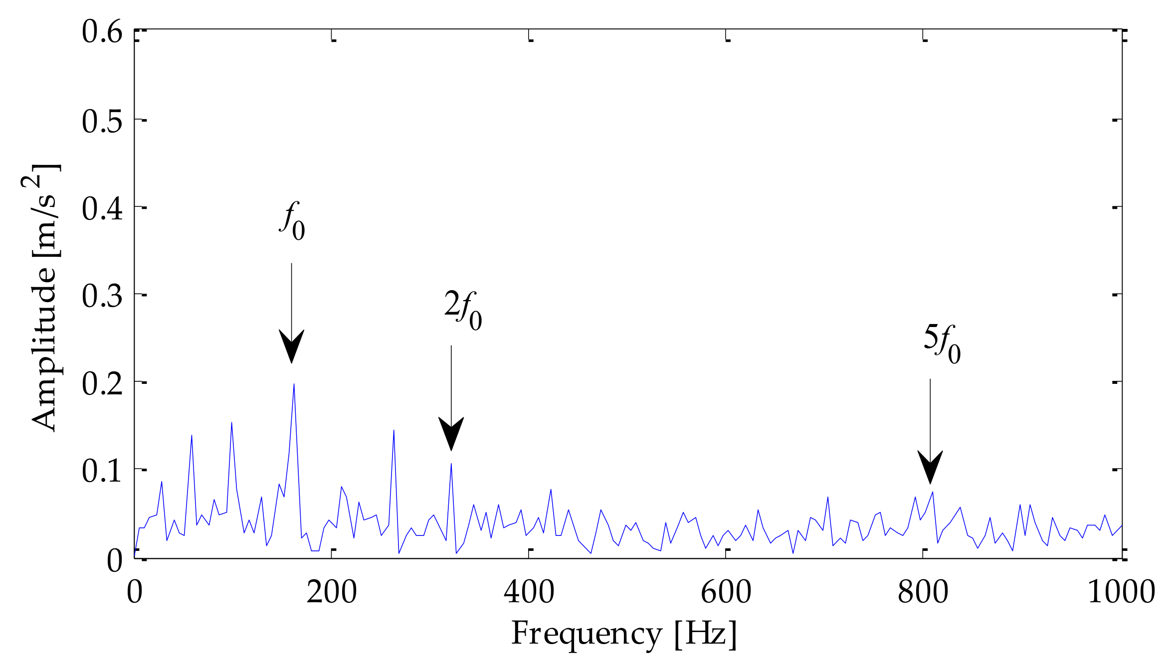
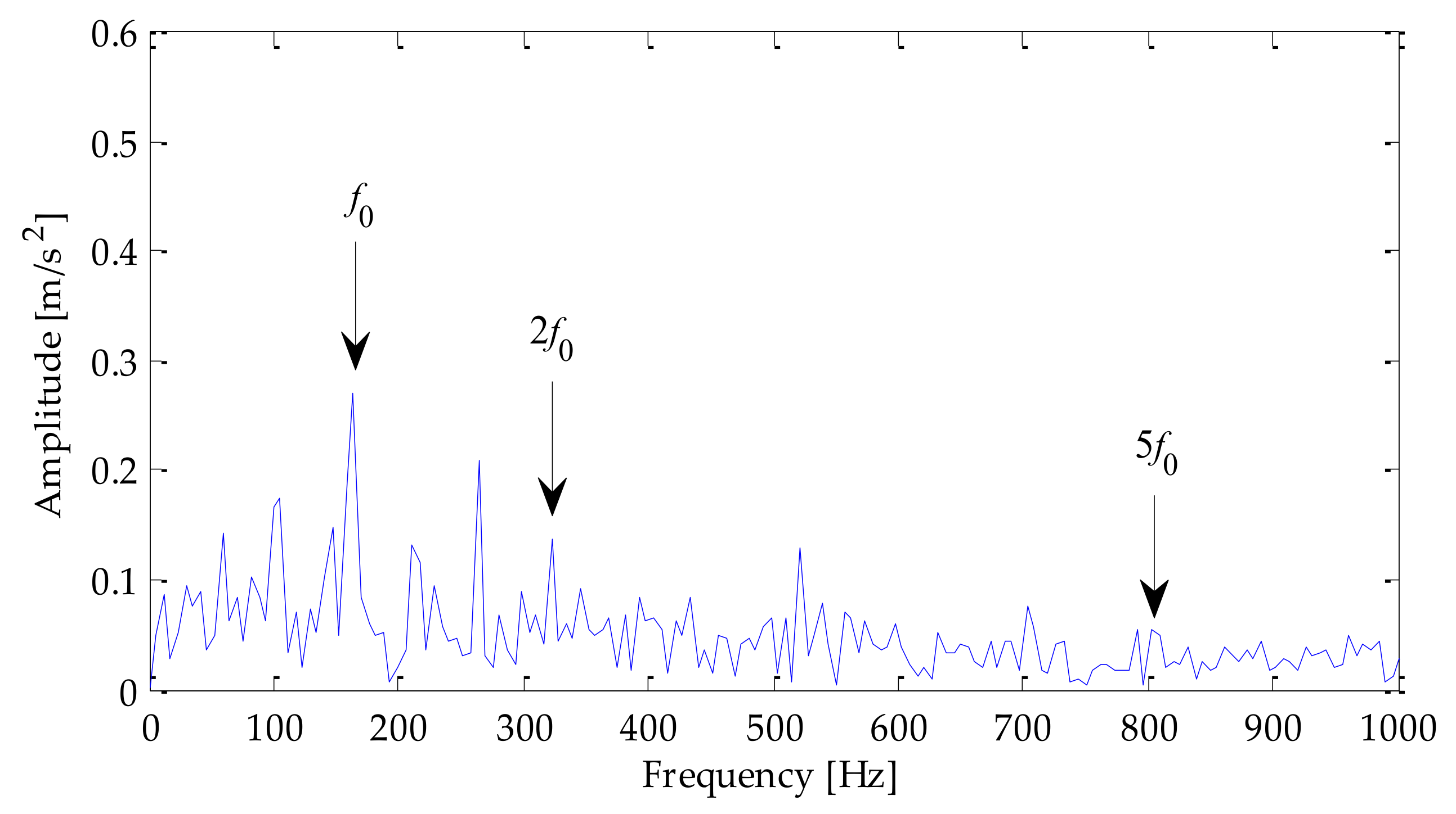
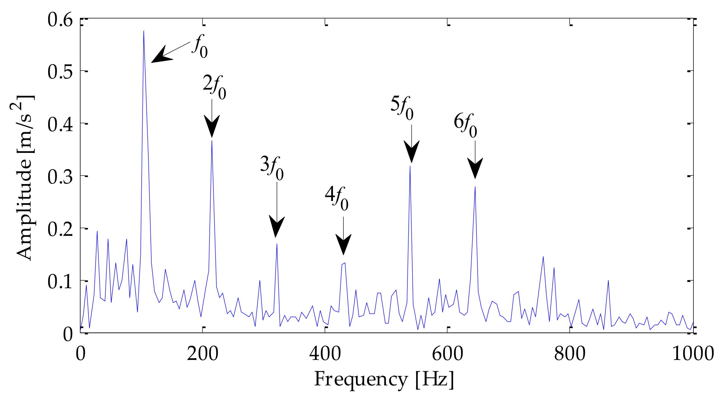
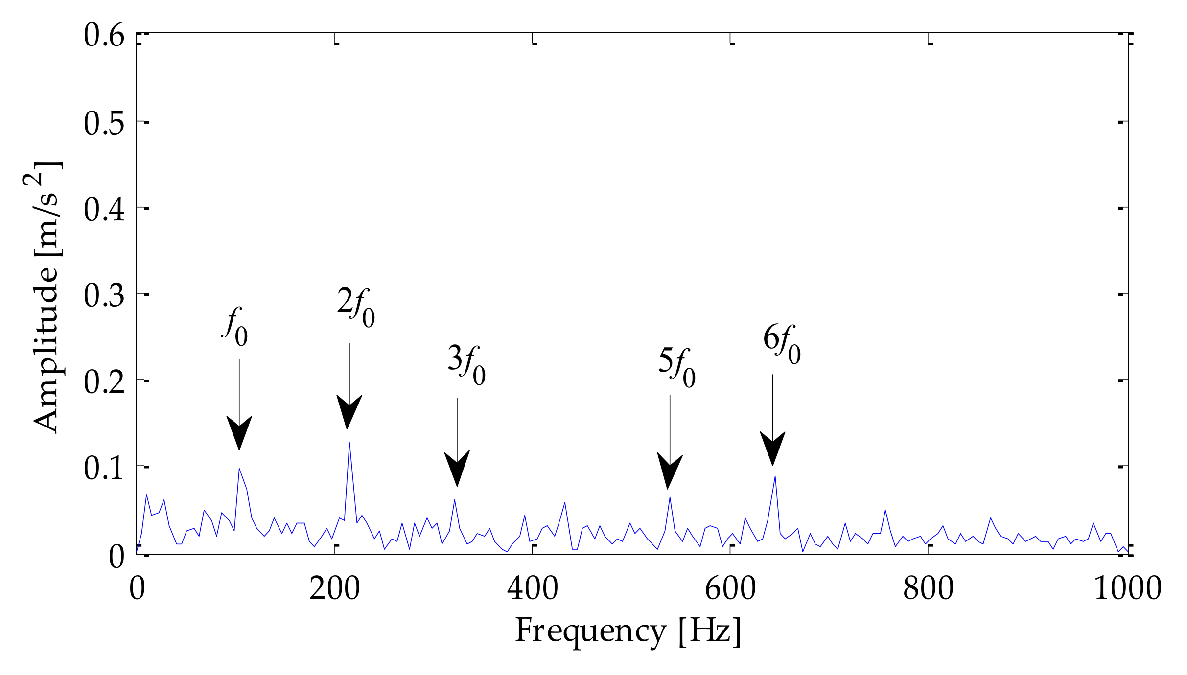
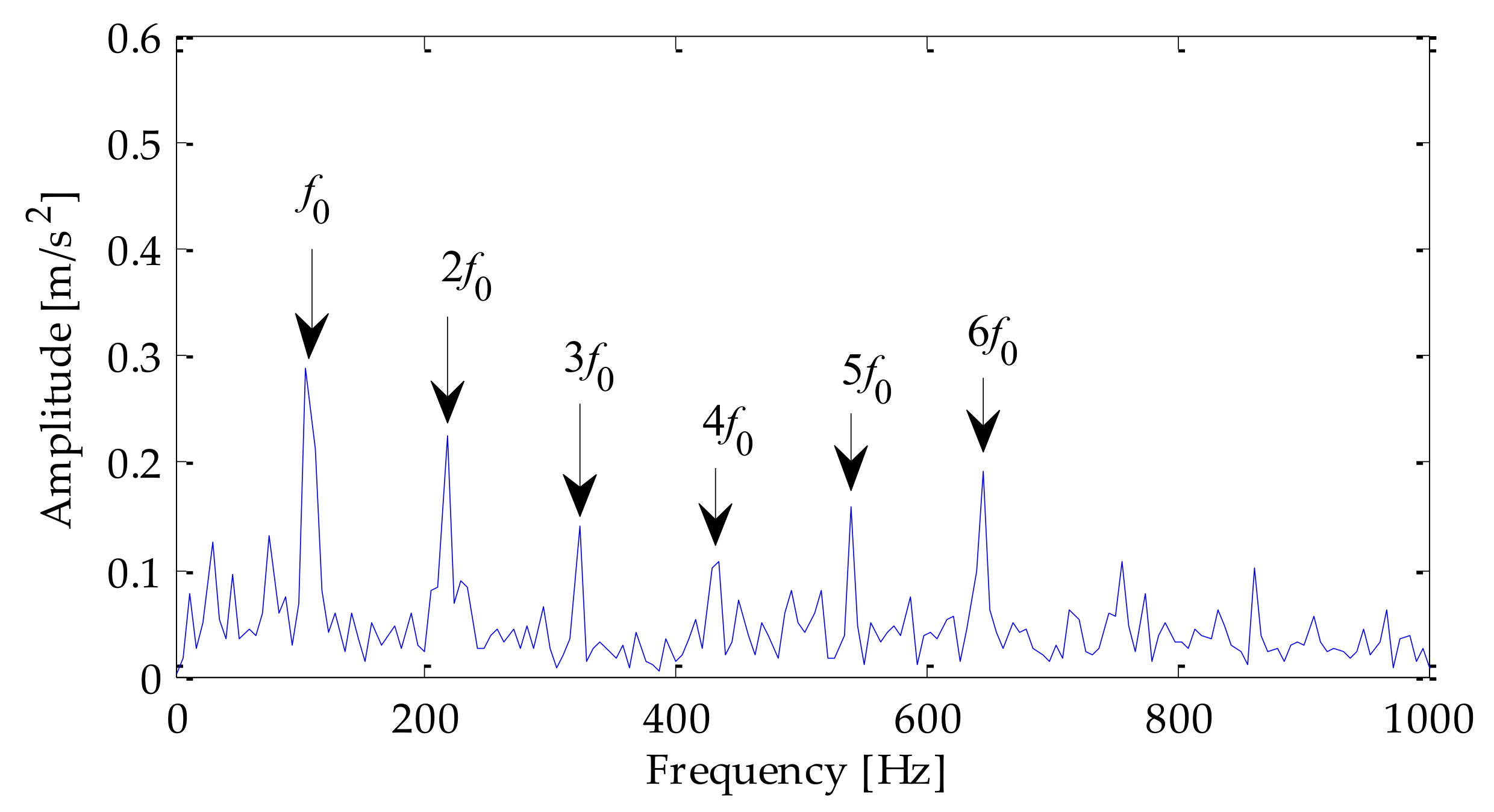
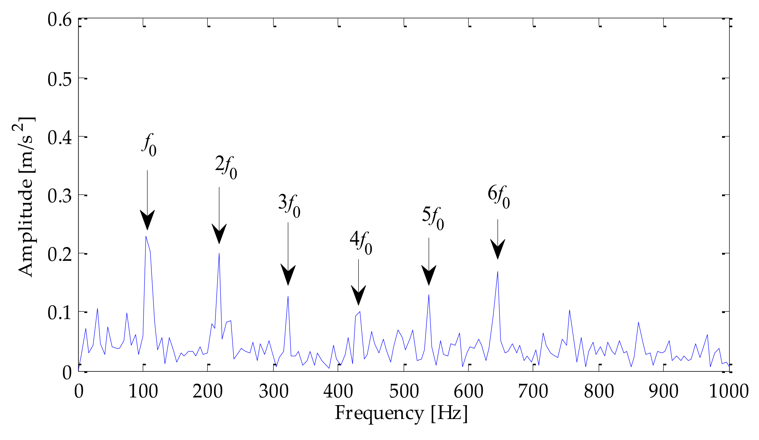
Next, Hilbert envelope demodulation was performed on the results obtained based on the above three methods, and then the corresponding fault features were extracted. The envelope spectrum is shown in Figure 16, Figure 17, Figure 18 and Figure 19. It can be seen from Figure 16 that the envelope spectrum obtained by the method proposed in this paper can clearly show multiple peaks with higher amplitudes, and the above peaks correspond to the frequency of one to eight times of the fault frequency, and so on. It shows that the useful signal and noise have been separated well, and the fault feature can be successfully extracted. At the same time, it can be seen from Figure 17, Figure 18 and Figure 19 that the envelope spectrum obtained by the LMD–RobustICA, EMD–RobustICA, and EEMD–RobustICA can extracted components such as two to eight times of the fault frequency. However, it is difficult to clearly distinguish the fundamental frequency of fault frequency from each peak. In addition, compared with Figure 16, the amplitude of the fault frequency in Figure 17, Figure 18 and Figure 19 was relatively low. It can be seen that the effect of using the method proposed in this paper to extract fault features was more significant.

5. Case Analysis

To test whether the method proposed in this paper can effectively extract the fault characteristics of rolling bearing, an example was given to verify it. The experimental data used in the experiment were from Case Western Reserve University [33]. The structure diagram of the rolling bearing test platform and rolling bearing is shown in Figure 20 [31]. The experimental platform mainly consists of the drive motor, torque speed sensor, and power meter. Among them, the model of rolling bearing at the driving end was 6205-2RSJEMSKF. Its specific parameters are shown in

Table 6. The bearing structure factor.

Inner Diameter (Inches)	Outer Diameter (Inches)	Contact Angle (α)	Pitch Circle Diameter D (Inches)	Speed (rpm)
0.9843	2.0472	00	1.5327	1797

. During the experiment, the set sampling frequency was 12 KHz. The acceleration sensor collected the vibration signals of the inner and outer rings with a damage diameter of 0.007 inches for experimental analysis. By substituting the relevant parameters in Table 6 into the calculation formula of fault characteristic fundamental frequency of inner ring and outer ring of rolling bearing, it can be calculated that the fundamental frequency of inner ring fault was 162.19 Hz and that of outer ring fault was 107.36 Hz.

5.1. Inner Ring Signal Analysis

By processing the collected signal, the time domain waveform and frequency domain waveform of the fault signal of the inner ring of the rolling bearing are shown in Figure 21 and Figure 22 can be obtained. It can be seen from that the noise interference in the signal was relatively small, and the fault impact characteristics were prominent. To test the method’s effectiveness, SNR = −2 dB white Gaussian noise was added to the inner ring fault signal in this experiment. The time–domain waveform and frequency–domain waveform of the finally mixed signal is shown in Figure 23 and Figure 24, respectively.

Next, the fault signal of the inner ring of the rolling bearing after adding noise will be processed. Firstly, the VMD was optimized by information entropy to select the values of parameters α and k to be initialized in VMD. The default value of α was 2500. Then, we initialized k = 3, and the search range of k was set to [3,15]. The value of optimal mode k was searched according to the principle of minimum envelope spectral entropy. The relationship between k and envelope spectral entropy as shown in Figure 25 can be obtained through calculation. As can be seen from Figure 25, with the continuous increase of k value, the value of the corresponding envelope spectral entropy was first decreased, then gradually increased, and, finally, decreased. Therefore, k = 4 was taken as the optimal value.

Next, the value of α was determined by experiment. The search range of α was set as [100, 2500], and then the value of the optimal mode was searched according to the principle of minimum envelope spectral entropy. The relationship between α and envelope spectral entropy as shown in Figure 26 can be obtained through calculation. As the value of α increases, the corresponding envelope spectral entropy decreases and gradually tends to be flat. When α = 2050, the envelope spectrum entropy was the smallest. Therefore, the value of α was 2050. After the above parameter optimization, it can be obtained that the value of the optimal parameter combination k and α was [4, 2050].

Next, this experiment substituted the selected initialization parameters into VMD, and then decomposed the signal. As is shown in Figure 27, after VMD decomposition optimized by information entropy, four IMF components were obtained. Because VMD has excellent advantages in suppressing mode aliasing and endpoint effect, it has better signal characterization ability. Next, all signal components C(t) and Q(t) were calculated. The calculated results are shown in

Table 7. The correlation coefficient and kurtosis between IMFand original signal (VMD).

Parameter	IMF1	IMF2	IMF3	IMF4
C(t)	0.354	0.396	0.512	0.524
Q(t)	2.661	3.044	4.174	4.082

. It can be seen that the IMF1 component and IMF1 component obtained by VMD decomposition met the conditions for screening the optimal signal component. That is, C(t) was greater than 0.3, and Q(t) was more significant than 3. Therefore, the above two IMF components were selected to reconstruct the observation signal channel. Finally, on this basis, RobustICA algorithm was used to separate signal and noise. The signal noise-reduction results obtained by using the proposed method are shown in Figure 28. Some impact characteristics of the signal can already be shown in Figure 28.

Finally, the denoised signal was demodulated by the Hilbert envelope, and then the corresponding fault features were extracted. To compare the experimental effects of different methods, LMD–RobustICA, EMD–RobustICA, and EEMD–RobustICA were used to denoise the signal. Then Hilbert envelope spectrum was generated.The envelope spectra obtained based on the above three methods are shown in Figure 29, Figure 30, Figure 31 and Figure 32, respectively. After analyzing the above four graphs, it can be seen that from the envelope spectrum of the above methods, the one-time frequency of the fault frequency, as well as the two-time frequency and five-time frequency of the fault frequency could be extracted. However, the amplitude of the fault frequency in the envelope spectrum obtained based on the method proposed in this paper was relatively high, especially the fundamental frequency amplitude. Therefore, the effect of using the proposed method to extract fault features was more significant.

5.2. Outer Ring Signal Analysis

By extracting the rolling bearing outer ring fault signal data, the time domain waveform and frequency domain waveform of the outer ring fault signal is shown in Figure 33 and Figure 34. Similarly, SNR = −2 dB white Gaussian noise was added to the inner ring fault signal in this experiment to test the method’s effectiveness.The time domain waveform and frequency domain waveform of the finally obtained mixed signal are shown in Figure 35 and Figure 36. Due to noise interference, it wasnot easy to distinguish the impact features from the diagram. Next, the signal was further processed.

Next, the VMD was optimized by information entropy to select the parameters α and k was initialized. Similarly, the value of α was the default value of 2500. First, k = 3 was initialized, and the search range of k was set to [3,15]. The value of optimal mode kwas searched according to the principle of minimum envelope spectral entropy. Through the search, the results shown in Figure 37 can be obtained. It is shown that the corresponding envelope spectral entropy’s value increased with the continuous increase of the k value. Therefore, k = 3 was taken as the optimal value.

Based on the above calculation results, the value of α was searched. The search range of α was set as [100, 2500], and then the value of the optimal mode α was searchedaccording to the principle of minimum envelope spectral entropy. Through calculation, the relationship between α and envelope spectral entropy as shown in Figure 38 can be obtained. As shown in Figure 38, with the increasing value of α, the corresponding envelope spectral entropy was decreasing and gradually tends to be flat. When α = 1900, the envelope spectral entropy was the smallest. Therefore, the value of α was 2050. After the above parameter optimization, it can be obtained that the value of the optimal parameter combination k and α was [3, 1900].

Next, the optimal parameters obtained by the search were substituted into the VMD, and then the signal was decomposed. As is shown in Figure 39, after VMD decomposition optimized by information entropy, three IMFs were obtained. Based on the above decomposition results, the C(t) and Q(t) of IMF1, IMF2, and IMF3 are further calculated. The calculated results are shown in

Table 8. The correlation coefficient and kurtosis between IMFand original signal (VMD).

Parameter	IMF1	IMF2	IMF3
C(t)	0.363	0.489	0.623
Q(t)	2.894	3.373	4.323

. It can be seen that the IMF2 component and IMF3 component obtained by VMD decomposition met the conditions for screening the optimal signal component. That is, C(t) was greater than 0.3 and Q(t) was more significant than 3. Therefore, the above two signal components were selected and used to reconstruct the observation signal channel. Then, RobustICA was used for signal noise reduction. The final signal noise-reduction result is shown in Figure 40. It can be seen that the periodic impact had a high similarity with the waveform of the original signal.

Next, the outer ring fault signal after signal noise reduction was demodulated by the Hilbert envelope to extract the fault feature. To furtheranalyze the fault feature extraction effect of the proposed method more intuitively, LMD–RobustICA, EMD–RobustICA, and EMD–RobustICA methods were used to denoise the signal. Then Hilbert envelope spectrum was generated. The envelope spectra obtained based on the above methods are shown in Figure 41, Figure 42, Figure 43 and Figure 44, respectively. Through the analysis of Figure 41, Figure 42, Figure 43 and Figure 44, it can be seen that the frequency doubling component of the outer ring fault characteristic frequency could be extracted by using the above methods for fault feature extraction. Meanwhile, the peak value of the components of the fault frequency from one to six times frequency is much higher than that obtained by the other three methods. The surrounding interference could not affect the identification of frequency doubling. However, the peak value of fault characteristic frequency in the envelope spectrum based on the other three methods was relatively low, and the interference components near these frequencies were close to the fault characteristic frequency. This brought some interference to fault feature extraction.

6. Conclusions

In this paper, a fault feature extraction of the rolling bearing signal under strong noise background is studied by using the combination of VMD optimized with information entropy and RobustICA. The conclusions were as follows.

(1) Although VMD can analyze the signal in the frequency domain, the effect is limited by the impact of modal component k and penalty factor α. This study used information entropy to optimize VMD to set initialization parameters. Compared with the way of setting parameters by experience, this method can search for a better combination of VMD parameters. This method can overcome the problems of modal aliasing and endpoint effect caused by impact component and noise interference in traditional EMD, LMD and EEMD, and has a good processing effect on the extraction of fault characteristic frequency of non-stationary and nonlinear signals. It can extract fault features more accurately. Compared with the traditional method, the experimental results show that this method can highlight the fault characteristic frequency and distinguish the fault.

(2) In this experiment, a typical simulation signal model is selected and Gaussian white noise is added on this basis to simulate the periodic impact signal caused by bearing fault under the condition of noise interference. Then, a signal component screening criterion based on correlation coefficient and kurtosis is established, and the optimal signal component is used to construct the observation signal channel of RobustICAalgorithm, so as to achieve the purpose of noise reduction.Through the in-depth analysis of the constructed simulation signal and the collected signal of the actual rolling bearing, it can be seen that compared with the traditional methods based on LMD–RobustICA, EMD–RobustICA, and EEMD–RobustICA, the method proposed in this paper can obtain better evaluation results of noise-reduction index, and the time–domain waveform of the signal after noise reduction is very similar to the waveform of the original signal.

(3) By comparing and analyzing the envelope demodulation results obtained by different methods, it can be seen that after the envelope spectrum analysis using the method proposed in this paper, the amplitude of fault characteristic frequency has been enhanced, and the surrounding interference will not affect the identification of fault fundamental frequency and frequency doubling, which is more convenient for fault diagnosis and analysis.

As an effective adaptive signal processing method, VMD has achieved good results in the field of fault diagnosis. However, the relevant parameters of this method need to be set in advance. In the process of parameter optimization, there is no theoretical basis for the definition of parameter search range. Therefore, in the next work, we will conduct in-depth research and further improve the parameter optimization method of VMD method.

References

1. Griffin, D.W.; Lim, J.S. Signal estimation from modified short-time Fourier transform. IEEE Trans. Acoust. Speech Signal Process. 1984, 32, 236–243. [Google Scholar] [CrossRef]
2. Kwok, H.K.; Jones, D.L. Improved instantaneous frequency estimation using an adaptive short-time Fourier transform. IEEE Trans. Signal Process. 2015, 48, 2964–2972. [Google Scholar] [CrossRef]
3. Stockwell, R.G.; Mansinha, L.; Lowe, R.P. Localization of the complex spectrum: The S transform. IEEE Trans. Signal Process. 1996, 44, 998–1001. [Google Scholar] [CrossRef]
4. Boashash, B.; Black, P.J. An efficient real-time implementation of the Wigner-Ville distribution. IEEE Trans. Acoust. Speech Signal Process. 1987, 35, 1611–1618. [Google Scholar] [CrossRef]
5. Morlet, J.; Arens, G.; Fourgeau, E.; Glard, D. Wave propagation and sampling theory 1: Complex signal and scattering in multilayered media. Geophysics 1982, 47, 203–221. [Google Scholar] [CrossRef] [Green Version]
6. Hazarika, N.; Chen, J.Z.; Tsoi, A.C.; Sergejew, A.A. Wavelet Transform. Signal Process. 1997, 59, 61–72. [Google Scholar] [CrossRef]
7. Bonizzi, P.; Karel, J.M.; Meste, O.; Peeters, R.L.M. Singular spectrum decomposition: A new method for time series decomposition. Adv. Adapt. Data Anal. 2014, 6, 1450011. [Google Scholar] [CrossRef]
8. Saidi, L.; Ali, J.B.; Bechhoefer, E.; Benbouzid, M. Wind turbine high-speed shaft bearings health prognosis through a spectral kurtosis-derived indices and SVR. Appl. Acoust. 2017, 20, 1–8. [Google Scholar] [CrossRef]
9. Meng, L.; Xiang, J.; Zhong, Y.; Song, W. Fault diagnosis of rolling bearing based on second generation wavelet denoising and morphological filter. J. Mech. Sci. Technol. 2015, 29, 3121–3129. [Google Scholar] [CrossRef]
10. Muruganatham, B.; Sanjith, M.; Krishnakumar, B.; Murty, S.A.V.S. Roller element bearing fault diagnosis using singular spectrum analysis. Mech. Syst. Signal Process. 2013, 35, 150–166. [Google Scholar] [CrossRef]
11. Huang, N.E.; Shen, Z.; Long, S.R.; Wu, M.C.; Shih, H.H.; Zheng, Q.; Yen, N.-C.; Tung, C.C.; Liu, H.H. The empirical mode decomposition and the Hilbert spectrum for nonlinear and non-stationary time series analysis. Proc. Math. Phys. Eng. Sci. 1998, 454, 903–995. [Google Scholar] [CrossRef]
12. Yeh, J.R.; Shieh, J.S.; Huang, N.E. Ensemble empirical mode decomposition: A noise-assisted data analysis method. Adv. Adapt. Data Anal. 2010, 2, 135–156. [Google Scholar] [CrossRef]
13. Smith, J.S. The local mean decomposition and its application to EEG perception data. J. R. Soc. Interface 2005, 2, 443–454. [Google Scholar] [CrossRef] [PubMed]
14. Jiang, Z.; Wu, Y.; Li, J.; Liu, Y.; Wang, J.; Xu, X. Application of EMD and 1.5-dimensional spectrum in fault feature extraction of rolling bearing. J. Eng. 2019, 2019, 8843–8847. [Google Scholar] [CrossRef]
15. Fan, H.; Shao, S.; Zhang, X.; Wan, X.; Cao, X.; Ma, H. Intelligent Fault Diagnosis of Rolling Bearing Using FCM Clustering of EMD-PWVD Vibration Images. IEEE Access 2020, 8, 145194–145206. [Google Scholar] [CrossRef]
16. Hou, J.; Wu, Y.; Gong, H.; Ahmad, A.S.; Liu, L. A Novel Intelligent Method for Bearing Fault Diagnosis Based on EEMD Permutation Entropy and GG Clustering. Appl. Sci. 2020, 10, 386. [Google Scholar] [CrossRef] [Green Version]
17. Liang, J.; Wang, L.; Wu, J.; Liu, Z. Elimination of End effects in LMD Based on LSTM Network and Applications for Rolling Bearing Fault Feature Extraction. Math. Probl. Eng. 2020, 2020, 7293454. [Google Scholar] [CrossRef]
18. Dragomiretskiy, K.; Zosso, D. Variational Mode Decomposition. IEEE Trans. Signal Process. 2014, 62, 531–544. [Google Scholar] [CrossRef]
19. Ye, M.; Yan, X.; Jia, M. Rolling Bearing Fault Diagnosis Based on VMD-MPE and PSO-SVM. Entropy 2021, 23, 762. [Google Scholar] [CrossRef]
20. Li, X.; Ma, Z.; Kang, D.; Li, X. Fault diagnosis for rolling bearing based on VMD-FRFT. Measurement 2020, 155, 107554. [Google Scholar] [CrossRef]
21. Xing, T.T.; Zeng, Y.; Meng, Z.; Guo, X. A fault diagnosis method of rolling bearing based on VMD Tsallis entropy and FCM clustering. Multimed. Tools Appl. 2020, 79, 30069–30085. [Google Scholar]
22. Albataineh, Z.; Salem, F.M. ARobustICA-based algorithmic system for blind separation of convolutive mixtures. Int. J. Speech Technol. 2021, 24, 701–713. [Google Scholar] [CrossRef]
23. Li, Q.; Li, M.; Zhang, X.; Ba, W. Research on Mixed Signal Separation method for Pipeline Leakage Based on RobustICA. In Proceedings of the International Conference on Robotics & Automation Engineering, Jeju, Korea, 27–29 August 2016; IEEE: Washington, DC, USA, 2016; pp. 70–74. [Google Scholar]
24. Yao, J.; Xiang, Y.; Qian, S.; Zhang, G. Cylinder Head Vibration Signals Separation of Internal Combustion Engines Based on VMD and RobustICA. China Mech. Eng. 2018, 29, 923–929. [Google Scholar]
25. Yang, J.Z.; Wang, X.D.; Feng, Z. A Noise Reduction Method Based on CEEMD-RobustICA and Its application in Pipeline Blockage Signal. J. Appl. Sci. Eng. 2019, 22, 1–10. [Google Scholar]
26. Yao, J.; Xiang, Y.; Qian, S.; Wang, S. Radiation Noise Separation of Internal Combustion Engine Based on Gammatone-RobustICA Method. Shock. Vib. 2017, 2017, 7565041. [Google Scholar] [CrossRef] [Green Version]
27. Zhao, F.; Wu, M. Application of EEMD- RobustICA and prony algorithm in modes identification of power system low frequency oscillation. Acta Energ. Sol. Sin. 2019, 40, 2919–2929. [Google Scholar]
28. Shannon, C.E. A mathematical theory of communication. Bell Syst. Tech. J. 1948, 27, 379–423. [Google Scholar] [CrossRef] [Green Version]
29. Zarzoso, V.; Comon, P. Robust independent component analysis for blind source separation and extraction with application in electrocardiography. In Proceedings of the 30th Annual International Conference of the IEEE Engineering in Medicine and Biology Society, Vancouver, BC, Canada, 20–25 August 2008. [Google Scholar]
30. Zarzoso, V.; Comon, P. Robust independent component analysis by iterative maximization of the kurtosis contrast with algebraic optimal step size. IEEE Trans. Neural Netw. 2010, 21, 248–261. [Google Scholar] [CrossRef] [Green Version]
31. Yang, J.Z.; Li, X.F.; Wu, L.M. Research on Fault Feature Extraction Method Based on FDM-RobustICA and MOMEDA. Math. Probl. Eng. 2020, 2020, 6753949. [Google Scholar] [CrossRef]
32. Feng, Z.; Ma, J.; Wang, X.; Wu, J.; Zhou, C. An Optimal Resonant Frequency Band Feature Extraction Method Based on Empirical Wavelet Transform. Entropy 2019, 21, 135. [Google Scholar] [CrossRef] [Green Version]
33. Smith, W.A.; Randall, R.B. Rolling element bearing diagnostics using the Case Western Reserve University date: A benchmark study. Mech. Syst. Signal Process. Method 2015, 64, 100–131. [Google Scholar] [CrossRef]
Figure 1. Frame of independent component analysis.
Coatings 12 00419 g001
Figure 2. Parameter optimization process of VMD.
Coatings 12 00419 g002
Figure 3. Fault feature extraction method based on VMD optimized with information entropy and RobustICA.
Coatings 12 00419 g003
Figure 4. Time–domain waveform of the simulated signal.
Coatings 12 00419 g004
Figure 5. Time–domain waveform of the mixed signal.
Coatings 12 00419 g005
Figure 6. Frequency–domain waveform of the mixed signal.
Coatings 12 00419 g006
Figure 7. Curve of fitness varying with k value.
Coatings 12 00419 g007
Figure 8. Curve of fitness varying with α value.
Coatings 12 00419 g008
Figure 9. VMD decomposition result.
Coatings 12 00419 g009
Figure 10. LMD (a) andEMD (b) decomposition result.
Coatings 12 00419 g010
Figure 11. EEMD decomposition result.
Coatings 12 00419 g011
Figure 12. Noise-reduction results by the method proposed in this paper.
Coatings 12 00419 g012
Figure 13. LMD–RobustICA noise-reduction results.
Coatings 12 00419 g013
Figure 14. EMD–RobustICAnoise-reduction results.
Coatings 12 00419 g014
Figure 15. EEMD–RobustICAnoise-reduction results.
Coatings 12 00419 g015
Figure 16. Analysis of signal envelope spectrum after noise reduction based on the proposed method.
Coatings 12 00419 g016
Figure 17. Analysis of signal envelope spectrum after noise reduction based on LMD–RobustICA.
Coatings 12 00419 g017
Figure 18. Analysis of signal envelope spectrum after noise reduction based on EMD–RobustICA.
Coatings 12 00419 g018
Figure 19. Analysis of signal envelope spectrum after noise reduction based on EEMD–RobustICA.
Coatings 12 00419 g019
Figure 20. Illustration of the bearing experimental platform and rolling bearing. (a)Illustration of the bearing experimental platform. (b) Rolling bearing.
Coatings 12 00419 g020
Figure 21. Time–domain analysis of the inner ring fault signal.
Coatings 12 00419 g021
Figure 22. Frequency–domain analysis of the inner ring fault signal.
Coatings 12 00419 g022
Figure 23. Time domain analysis of the mixed signal.
Coatings 12 00419 g023
Figure 24. Frequency domain analysis of the mixed signal.
Coatings 12 00419 g024
Figure 25. Curve of fitness varying with K value.
Coatings 12 00419 g025
Figure 26. Curve of fitness varying with α value.
Coatings 12 00419 g026
Figure 27. VMD decomposition result.
Coatings 12 00419 g027
Figure 28. Noise-reduction results by the proposed method.
Coatings 12 00419 g028
Figure 29. Analysis of signal envelope spectrum after noise reduction based on the proposed method.
Coatings 12 00419 g029
Figure 30. Analysis of signal envelope spectrum after noise reduction based on LMD–RobustICA.
Coatings 12 00419 g030
Figure 31. Analysis of signal envelope spectrum after noise reduction based on EMD–RobustICA.
Coatings 12 00419 g031
Figure 32. Analysis of signal envelope spectrum after noise reduction based on EEMD–RobustICA.
Coatings 12 00419 g032
Figure 33. Time domain analysis of the outer ring fault signal.
Coatings 12 00419 g033
Figure 34. Frequency domain analysis of the outer ring fault signal.
Coatings 12 00419 g034
Figure 35. Time domain analysis of the mixed signal.
Coatings 12 00419 g035
Figure 36. Frequency domain analysis of the mixed signal.
Coatings 12 00419 g036
Figure 37. Curve of fitness varying with k value.
Coatings 12 00419 g037
Figure 38. Curve of fitness varying with a value.
Coatings 12 00419 g038
Figure 39. VMD decomposition result.
Coatings 12 00419 g039
Figure 40. Noise-reduction results by the proposed method.
Coatings 12 00419 g040
Figure 41. Analysis of signal envelope spectrum after noise reduction based on the proposed method.
Coatings 12 00419 g041
Figure 42. Analysis of signal envelope spectrum after noise reduction based on LMD–RobustICA.
Coatings 12 00419 g042
Figure 43. Analysis of signal envelope spectrum after noise reduction based on EMD–RobustICA.
Coatings 12 00419 g043
Figure 44. Analysis of signal envelope spectrum after noise reduction based on EEMD–RobustICA.
Coatings 12 00419 g044