
Research on the Quality of Asphalt Pavement Construction Based on Nondestructive Testing Technology

 ,
,
Abstract
:1. Introduction
2. Nondestructive Testing Equipment and Principles
2.1. Three-Dimensional Ground-Penetrating Radar (GPR)
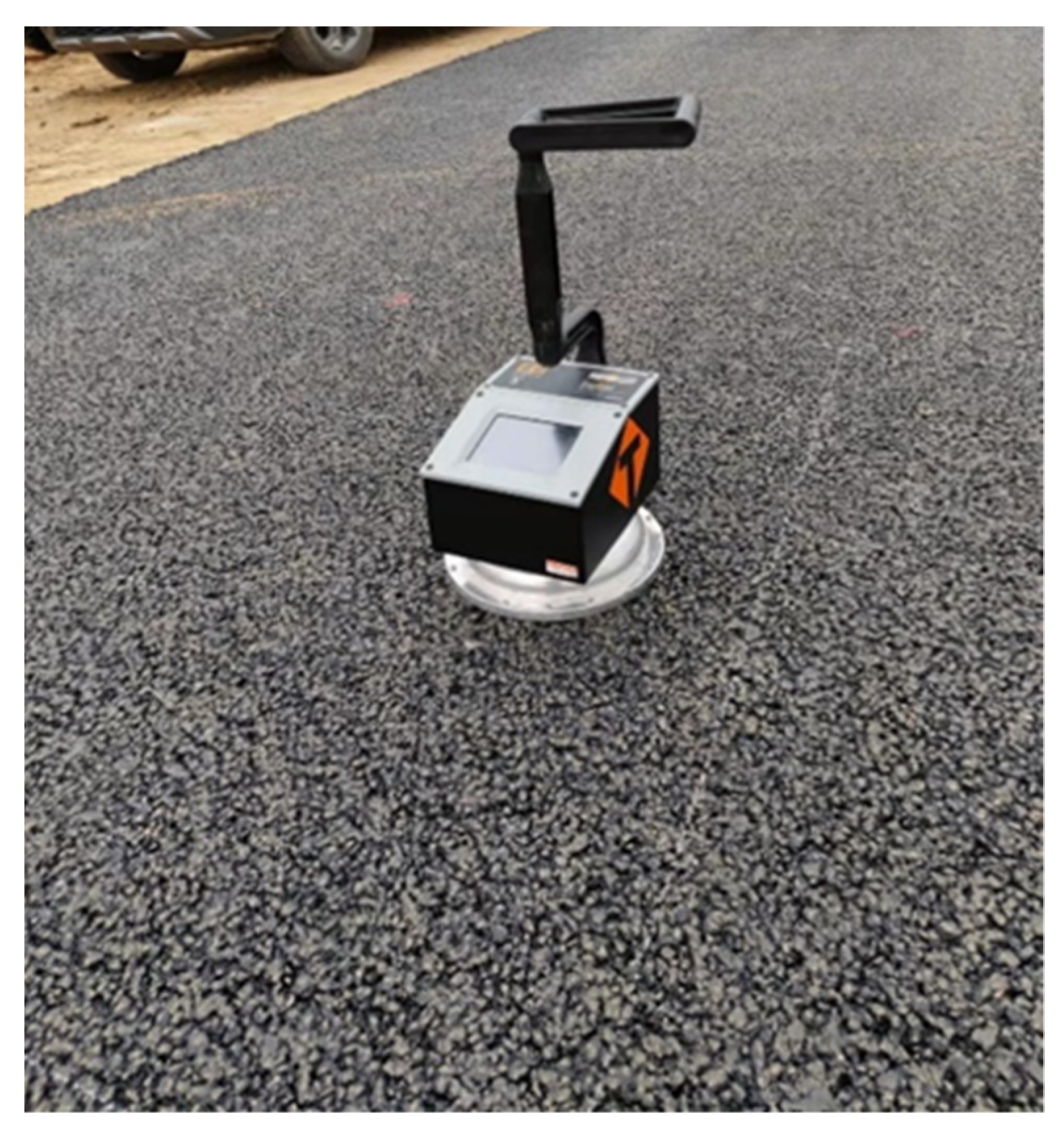
2.2. Non-Nuclear Density Gauge
2.3. Total Reflection Method
3. Selection of Representative Values for Ground-Penetrating Radar Dielectric Constants
3.1. Design of Scheme for Value of Dielectric Constant for Asphalt Mixture Pavements
3.1.1. Method 1
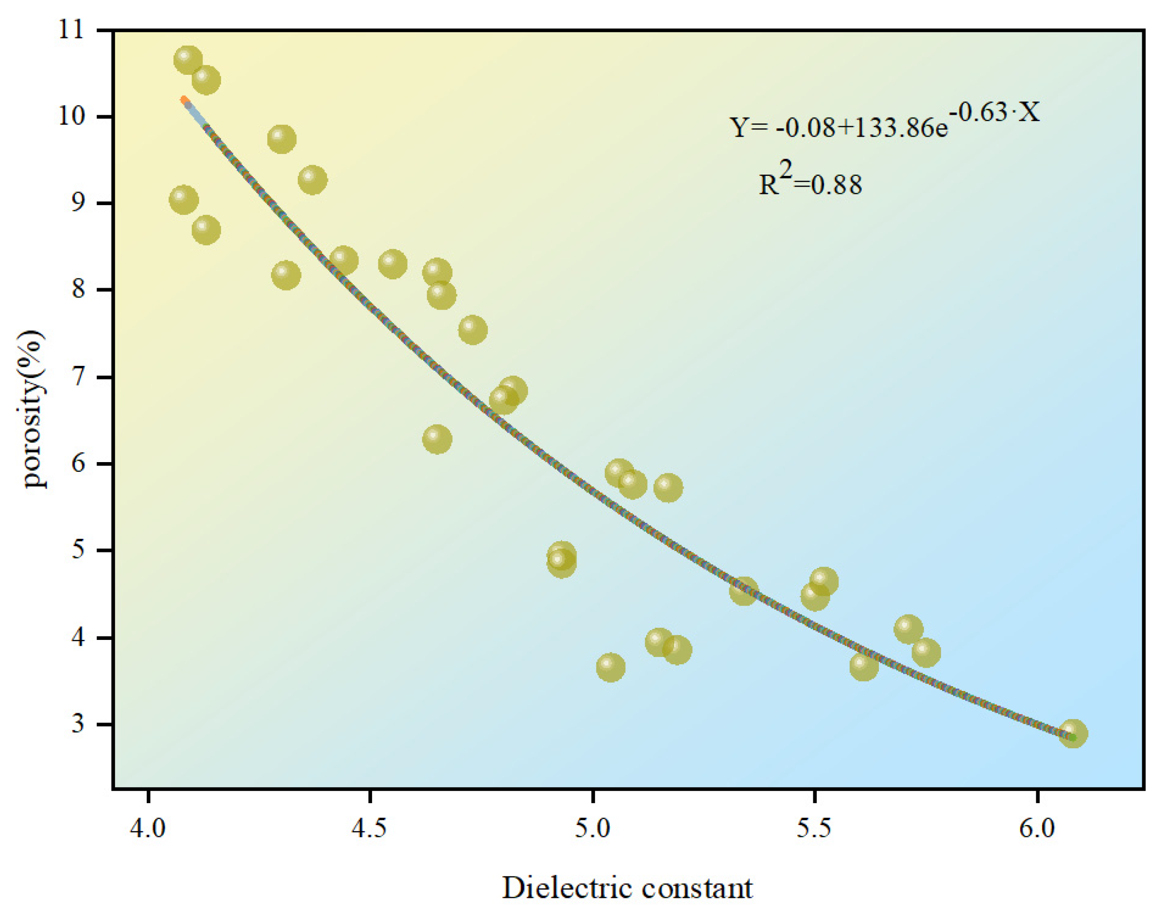
3.1.2. Method 2
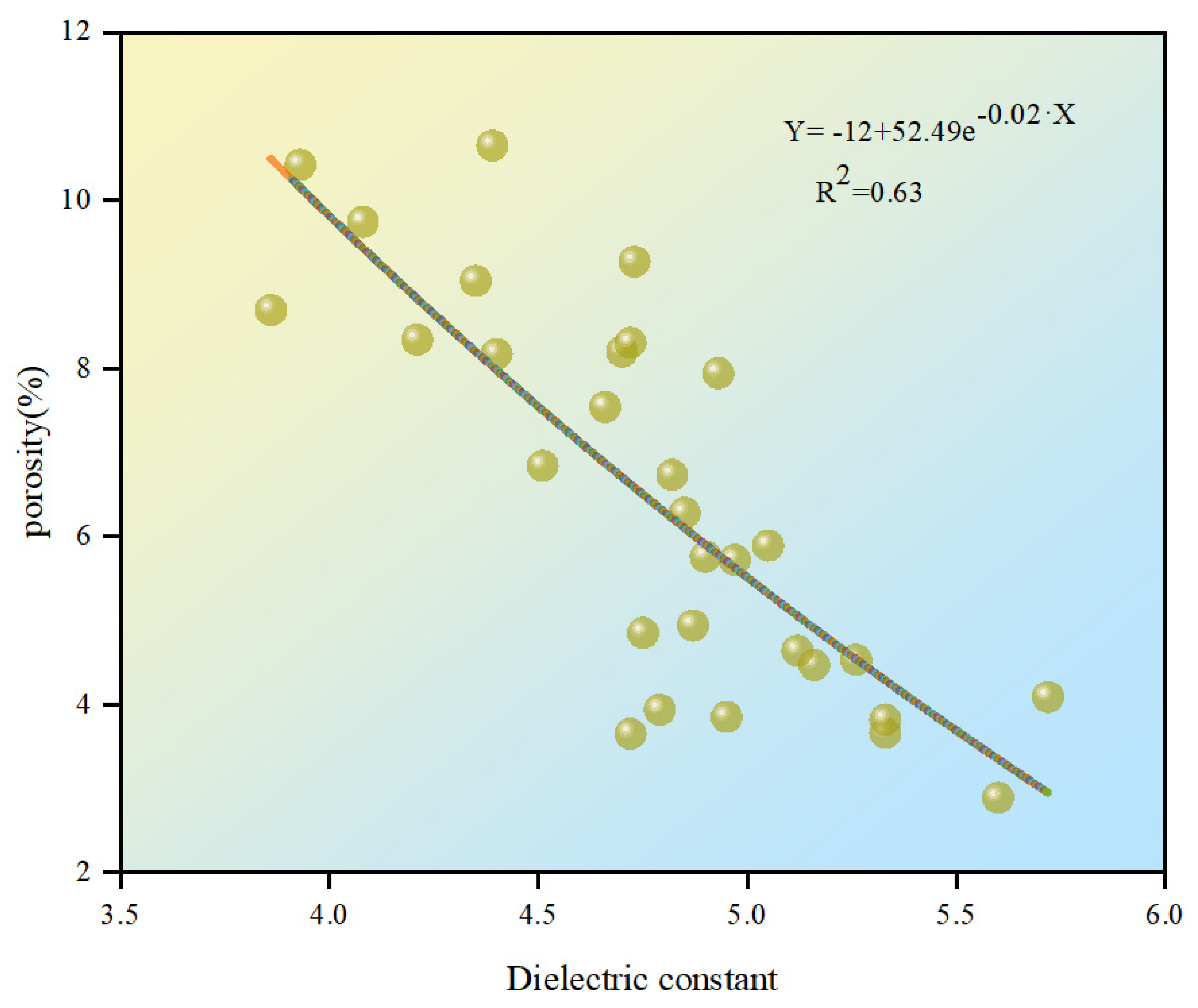
3.1.3. Method 3
3.2. Determination of Dielectric Constant Value Method of Asphalt Mixture Pavement
4. Asphalt Pavement Construction Quality Evaluation Study
4.1. Engineering Background
4.1.1. Materials
4.1.2. Grading Design of Asphalt Mixes
4.2. Experimental Design
4.3. Evaluation of Asphalt Pavement Construction Quality Based on PQI 380
4.4. Evaluation of Asphalt Pavement Construction Quality Based on GPR
5. Conclusions
Author Contributions
Funding
Institutional Review Board Statement
Informed Consent Statement
Data Availability Statement
Acknowledgments
Conflicts of Interest
References
- Wang, L. Significance analysis of influencing factors of highway freight transportation in China and multi-variable grey prediction for its development. J. Intell. Fuzzy Syst. 2021, 41, 1237–1246. [Google Scholar] [CrossRef]
- Sun, L.; Li, X.; Wang, X. Study on the damage of semi rigid base asphalt pavement under high temperature condition. In Proceedings of the 4th International Conference on Mechatronics, Materials, Chemistry and Computer Engineering 2015, Xi’an, China, 12–13 December 2015. [Google Scholar]
- Tutu, K.A.; Timm, D.H. A Recursive Pseudo Fatigue Cracking Damage Model for Asphalt Pavements. Int. J. Pavement Eng. 2018, 1–21. [Google Scholar] [CrossRef]
- Zhi, Z.; Dai, C.S.; Guo, S.Y. Study on risk early warning system of asphalt concrete pavement design. In Proceedings of the 2013 International Conference on Management Science and Engineering (ICMSE), Harbin, China, 17–19 July 2013. [Google Scholar]
- Nobakht, M.; Zhang, D.; Sakhaeifar, M.S.; Lytton, R.L. Characterization of the adhesive and cohesive moisture damage for asphalt concrete. Constr. Build. Mater. 2020, 247, 118616. [Google Scholar] [CrossRef]
- Scullion, S.T. Road evaluation with ground penetrating radar. J. Appl. Geophys. 2000, 43, 119–138. [Google Scholar]
- Solla, M.; González-Jorge, H.; Lorenzo, H.; Arias, P. Uncertainty evaluation of the 1GHz GPR antenna for the estimation of concrete asphalt thickness. Measurement 2013, 46, 3032–3040. [Google Scholar] [CrossRef]
- Chamberlain, A.T.; Sellers, W.; Proctor, C.; Coard, R. Cave Detection in Limestone using Ground Penetrating Radar. J. Archaeol. Sci. 2000, 27, 957–964. [Google Scholar] [CrossRef] [Green Version]
- Baltruaitis, A.; Vaitkus, A.; Smirnovs, J. Asphalt Layer Density and Air Voids Content: GPR and Laboratory Testing Data Reliance. Balt. J. Road Bridge Eng. 2020, 15, 93–110. [Google Scholar] [CrossRef]
- Loizos, A.; Georgiou, P.; Plati, C. A comprehensive approach for the assessment of HMA compactability using GPR technique. Near Surf. Geophys. 2016, 14, 117–126. [Google Scholar]
- Benedetto, A.; Tosti, F.; Ciampoli, L.B.; D’Amico, F. An overview of ground-penetrating radar signal processing techniques for road inspections. Signal Process. 2017, 132, 201–209. [Google Scholar] [CrossRef]
- Zhang, J.; Yang, X.; Li, W.; Zhang, S.; Jia, Y. Automatic detection of moisture damages in asphalt pavements from GPR data with deep CNN and IRS method. Autom. Constr. 2020, 113, 103119. [Google Scholar] [CrossRef]
- Ma, Y.; Elseifi, M.A.; Dhakal, N.; Bashar, M.Z.; Zhang, Z. Non-Destructive Detection of Asphalt Concrete Stripping Damage using Ground Penetrating Radar. Transp. Res. Rec. J. Transp. Res. Board 2021, 2675, 938–947. [Google Scholar] [CrossRef]
- Loizos, A.; Plati, C. Accuracy of pavement thicknesses estimation using different ground penetrating radar analysis approaches. NDT E Int. 2007, 40, 147–157. [Google Scholar] [CrossRef]
- Shangguan, P.; Alqadi, I.L.; Leng, Z.; Schmitt, R.; Faheem, A. An Innovative Approach for Asphalt Pavement Compaction Monitoring Using Ground Penetrating Radar. Transp. Res. Rec. J. Transp. Res. Board 2013, 2347, 79–87. [Google Scholar] [CrossRef]
- Plati, C.; Loizos, A. Using ground-penetrating radar for assessing the structural needs of asphalt pavements. Nondestruct. Test. Eval. 2012, 27, 273–284. [Google Scholar] [CrossRef]
- Shangguan, P.; Al-Qadi, I.L. Calibration of FDTD Simulation of GPR Signal for Asphalt Pavement Compaction Monitoring. IEEE Trans. Geosci. Remote Sens. 2014, 53, 1538–1548. [Google Scholar] [CrossRef]
- Praticò, F.G.; Moro, A.; Ammendola, R. Factors Affecting Variance and Bias of Non-nuclear Density Gauges for Porous European Mixes and Dense-Graded Friction Courses. Balt. J. Road Bridge Eng. 2009, 4, 99–107. [Google Scholar] [CrossRef]
- Van den Bergh, V.; Vuye, C.; Kara, P.; Couscheir, K.; Blom, J.; Van Bouwel, P. The use of a non-nuclear density gauge for monitoring the compaction process of asphalt pavement. IOP Conf. Ser. Mater. Sci. Eng. 2017, 236, 012014. [Google Scholar] [CrossRef] [Green Version]
- Fernandes, F.M.; Pais, J.C. Virtual Special Issue Ground-Penetrating Radar and Complementary Non-Destructive Testing Techniques in Civil Engineering Laboratory observation of cracks in road pavements with GPR. Constr. Build. Mater. 2017, 154, 1130–1138. [Google Scholar] [CrossRef]
- Keefe, B.J. Permanent International Association of Road Congresses (PIARC): Report on the XVII World Road Congress Held in Sydney, October 1983. Qld. Roads 1983, 22, 44. [Google Scholar]
- Olhoeft, G.R. Applications and frustrations in using ground penetrating radar. IEEE Aerosp. Electron. Syst. Mag. 2002, 17, 12–20. [Google Scholar] [CrossRef] [Green Version]
- Cho, Y.; Wang, C.; Zhuang, Z. Framework for Empirical Process to Improve Nonnuclear Gauge Performance in Hot-Mix Asphalt Pavement Construction. J. Constr. Eng. Manag. ASCE 2013, 139, 601–610. [Google Scholar] [CrossRef]
- Sihvola, A.; Lindell, I.V. Polarizability and Effective Permittivity of Layered and Continuously Inhomogeneous Dielectric Spheres. J. Electromagn. Waves Appl. 1988, 4, 1–26. [Google Scholar] [CrossRef]
- Al-Qadi, I.; Lahouar, S.; Loulizi, A. Successful Application of Ground-Penetrating Radar for Quality Assurance-Quality Control of New Pavements. Transp. Res. Rec. J. Transp. Res. Board 2003, 1861, 86–97. [Google Scholar] [CrossRef]
- Wang, L.; Wang, Y.; Mohammad, L.; Harman, T. Voids Distribution and Performance of Asphalt Concrete. Int. J. Pavements 2002, 1, 22–33. [Google Scholar]
- JTG E20-2011; Standard Test Methods of Bitumen and Bituminous Mixtures for Highway Engineering. Ministry of Transport, China: Beijing, China, 2011.
- JTG F40-2004; Technical Specifications for Construction of Highway Asphalt Pavements. Ministry of Transport, China: Beijing, China, 2004.
- Li, X.; Zhou, Z.; Lv, X.; Xiong, K.; Wang, X.; You, Z. Temperature segregation of warm mix asphalt pavement: Laboratory and field evaluations. Constr. Build. Mater. 2017, 136, 436–445. [Google Scholar] [CrossRef]


| Method 1 | Method 2 | Method 3 | |
|---|---|---|---|
| Fitting equation | Y = 21.52 − 5.4e0.2·X | Y = −0.08 + 133.86e−0.63·X | Y = −12 + 52.49e−0.02·X |
| R2 | 0.54 | 0.88 | 0.63 |
| Items | Test Values | Specification [28] |
|---|---|---|
| Penetration (25 °C, 0.1 mm) | 52 | 40–60 |
| Ductility (5 °C, cm) | 29.3 | ≥20 |
| Softening point (°C) | 74 | ≥60 |
| Kinematic viscosity (135 °C, Pa.s) | 1.80 | ≤3 |
| Items | Unit | Limestone Test Results | Specification [28] |
|---|---|---|---|
| Apparent relative density | g/cm3 | 2.686 | ≥2.50 |
| Water absorption | % | 0.97 | ≤3.0 |
| Crush value | % | 23.1 | ≤28 |
| Abrasion value | % | 21.6 | ≤30 |
| Soundness | % | 7.0 | ≤12 |
| Items | Unit | Test Values | Specification [28] |
|---|---|---|---|
| Apparent relative density | g/cm3 | 2.726 | ≥2.5 |
| Sand equivalent | % | 78 | ≥60 |
| Soundness | % | 14 | ≥12 |
| Angularity | s | 49 | ≥30 |
| Percentage of Mass Passing the following Sieve Holes (%) | |||||||||||
|---|---|---|---|---|---|---|---|---|---|---|---|
| Items | 19 mm | 16 mm | 13.2 mm | 9.5 mm | 4.75 mm | 2.36 mm | 1.18 mm | 0.6 mm | 0.3 mm | 0.15 mm | 0.075 mm |
| Upper limit of gradation | 100 | 92 | 80 | 72 | 56 | 44 | 33 | 24 | 17 | 13 | 7 |
| Lower limit of gradation | 90 | 78 | 62 | 50 | 26 | 16 | 12 | 8 | 5 | 4 | 3 |
| Production mixture ratio | 94.6 | 84.4 | 74.4 | 59.2 | 37.6 | 25.2 | 17.8 | 13.0 | 9.8 | 7.5 | 5.4 |
| Core Sample 1 | Core Sample 2 | Core Sample 3 | |
|---|---|---|---|
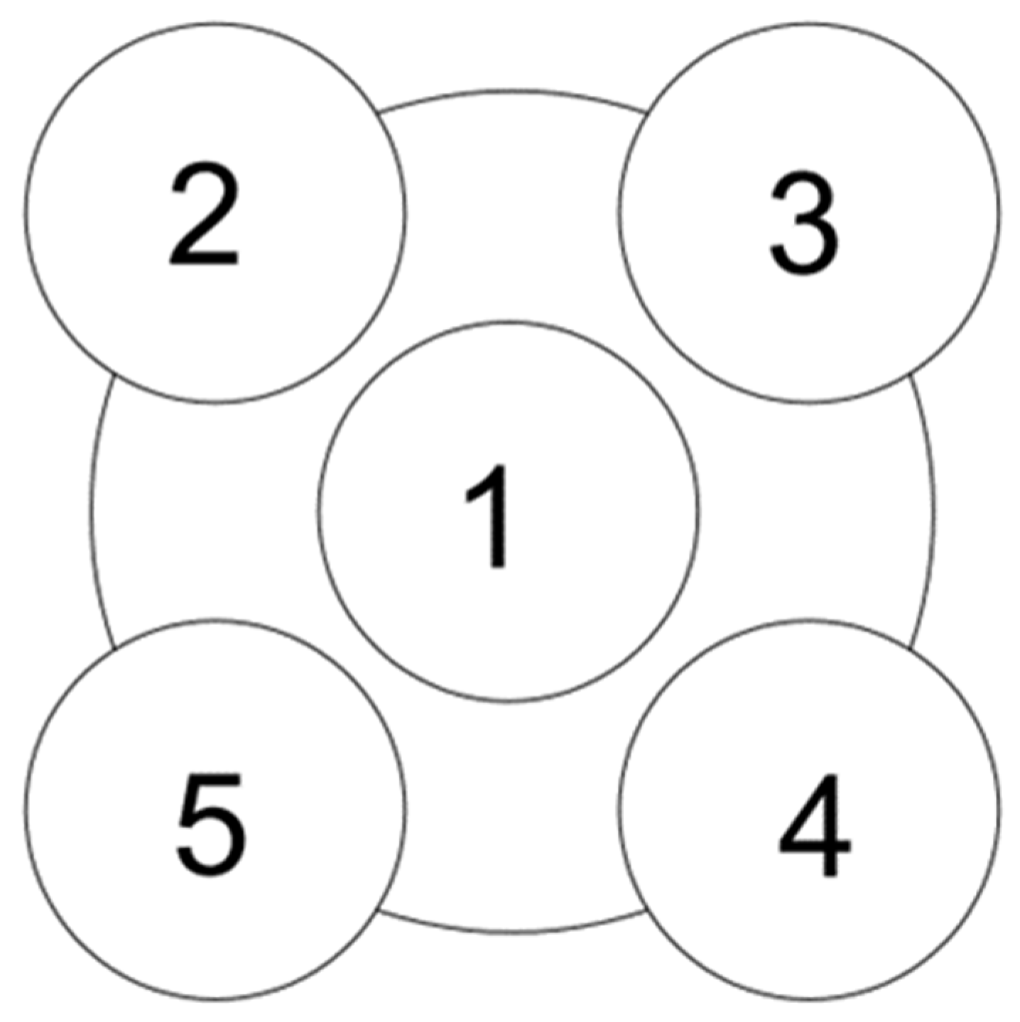
| Center Point 1 | 2.3725 | 2.3651 | 2.3656 |
| Center Point 2 | 2.3967 | 2.3854 | 2.3895 |
| Center Point 3 | 2.4661 | 2.3962 | 2.3864 |
| Center Point 4 | 2.3732 | 2.3979 | 2.3997 |
| Center Point 5 | 2.3822 | 2.3921 | 2.4123 |
| Average | 2.3981 | 2.3873 | 2.3907 |
| Measured core density | 2.396 | 2.413 | 2.446 |
| Correction factor | 0.9991 | 1.0107 | 1.0231 |
| Average of correction factors | 1.011 | ||
Publisher’s Note: MDPI stays neutral with regard to jurisdictional claims in published maps and institutional affiliations. |
© 2022 by the authors. Licensee MDPI, Basel, Switzerland. This article is an open access article distributed under the terms and conditions of the Creative Commons Attribution (CC BY) license (https://creativecommons.org/licenses/by/4.0/).
Share and Cite
Chen, W.; Hu, G.; Han, W.; Zhang, X.; Wei, J.; Xu, X.; Yan, X. Research on the Quality of Asphalt Pavement Construction Based on Nondestructive Testing Technology. Coatings 2022, 12, 379. https://doi.org/10.3390/coatings12030379
Chen W, Hu G, Han W, Zhang X, Wei J, Xu X, Yan X. Research on the Quality of Asphalt Pavement Construction Based on Nondestructive Testing Technology. Coatings. 2022; 12(3):379. https://doi.org/10.3390/coatings12030379
Chicago/Turabian StyleChen, Wei, Guiling Hu, Wenyang Han, Xiaomeng Zhang, Jincheng Wei, Xizhong Xu, and Xiangpeng Yan. 2022. "Research on the Quality of Asphalt Pavement Construction Based on Nondestructive Testing Technology" Coatings 12, no. 3: 379. https://doi.org/10.3390/coatings12030379