Maintenance Time of Permeable Asphalt Pavement Based on Entropy–Analytic Hierarchy Process Analysis

Abstract

Dust, sediment, and stone chips often block the rainwater-infiltration paths of permeable pavements, which, in conjunction with vehicle load, reduces drainage capacity. To restore this capacity, a reasonable maintenance time and suitable maintenance measures must be determined. Therefore, we investigated the void attenuation and decline in drainage capacity of permeable asphalt pavements under the combined action of dust blockage and vehicle load. First, the water seepage coefficient decay and the decay rate under blocking and compaction were determined via clogging and compaction experiments. Second, experimental data were incorporated into an entropy–analytic hierarchy process analysis model, with the gross domestic product ratio, wind scale, and maximum five-year rainfall for the area. Finally, three test roads were studied as the weight to rank the maintenance urgency and predict the maintenance timing for each road under different rainfall conditions. The results demonstrate that the drainage capacity of permeable pavements obeys the parabolic exponential attenuation law. From the findings regarding road water storage capacity, the latest pavement maintenance time at different rainfall levels were obtained. This predicted maintenance time enables better decisions than regular time on code, which is the effect of drainage caused by multiple factors.

1. Introduction

Permeable asphalt pavements are usually provided with large gaps, which permit rainwater to flow inside the pavement and be drained through a side ditch; this improves driving safety in the rain [1,2,3]. However, dust, sediment, and stone chips enter these gaps, thus blocking the drainage path [4,5].

Permeable asphalt pavements provide effective drainage and service and usually have an open-graded friction course (OGFC) [6]. After 20 years of development, the OGFC has been improved considerably. However, due to the open grading and large voids in the OGFC, it cannot adopt a dense skeleton structure, and this reduces the durability of the pavement. Therefore, it is necessary to optimize the mix proportion of the OGFC. Kandhal et al. [7] found that the use of polymer-modified asphalt binder and coarse aggregate gradation can improve the road performance of the OGFC. Alvarez et al. [8] asserted that for the OGFC, the factors to be considered include volume fraction, structural parameters, mixing performance, and function, as well as permeability and anti-sliding performance. Alvarez et al. [9] proved that it is technically feasible to analyze the contact behavior between the aggregates according to the grading curve during the design of OGFC mix proportion. Mo et al. [10] reported that a small increase in asphalt content can significantly improve the service life of permeable asphalt pavements. These studies show that considerable scope for improvement exists with regard to the mix proportion design of the OGFC.

Moreover, the movement of vehicles [11] increases the density of the pavement structure, thus reducing its drainage capacity [12]. Therefore, permeable pavements with a significantly reduced drainage capacity must be repaired to restore the initial drainage capacity. Ensuring continuous drainage for permeable pavements is an engineering, economic, and technical prerequisite for the application of drainage pavements in road engineering [13]; therefore, the selection of a suitable maintenance time is an important factor.

Extensive research has been conducted on the causes of blockage in permeable pavements, as well as on the decay law of the water permeability coefficient. Kurihara et al. [14] studied the water permeability of a porous asphalt mixture with a porosity of 20% and compared the effects of blockage type and amount on the pavement’s water permeability. Evaluation of the porous asphalt mixture should include the initial drainage and anti-blocking capacities. Tan et al. [15] found a quadratic relationship between the permeability coefficient of a porous asphalt mixture and the mass of particles remaining in the specimen during the plugging process. Gonzalez et al. [16] showed that compaction has a significant impact on the permeability of porous asphalt pavements; when the degree of compaction is higher, the permeability coefficient of the pavement decreases. Erdem et al. [17] found that under the combined action of rainwater and vehicle loads, the porosity of the lower layer of porous asphalt pavements decreases most significantly. Moriyoshi et al. [18] observed porous asphalt pavement for 14 years; they found that the permeability coefficient gradually decreases after the road is opened to traffic and that it becomes stable after two years. The studies cited above show that particle blockage and changes in vehicle load have a significant influence on the drainage capacity of permeable asphalt pavements. Therefore, it is of great significance to explore the rule governing this relationship and determine an appropriate maintenance time for permeable asphalt pavements.

At present, the multi-objective optimization methods applied in this area predominantly include the entropy method and analytic hierarchy process (AHP). The entropy method can calculate the weight of each index according to its variation degree, which provides the basis for multi-index comprehensive evaluation. AHP can decompose complex systems and transform certain multi-objective and multi-criteria decision-making problems that are difficult to quantify accurately into multi-level decision-making problems.

Several studies have been conducted on the entropy method and AHP. Tang et al. [19] combined the entropy method with the extremum machine learning method to predict short-term photovoltaic power generation and achieved a significantly high prediction accuracy. In terms of fan optimization, Zhang et al. [20] selected three parameters as optimization variables, established the optimization function between optimization variables and multiple objectives using the entropy method, and obtained an optimization model.

Liu et al. [21] stated that AHP is a multi-criteria decision-making method with wide application prospects that can determine the criteria weight and priority of schemes in a structured manner. Yilmaz et al. [22] used AHP to determine the weight of each factor affecting sensitivity and combined the weighted scores to grade ecologically sensitive areas. Although the entropy and AHP methods are widely used for weighting, the entropy method sometimes contradicts the actual situation [23], whereas the AHP principal component analysis method relies excessively on subjective factors.

To obviate the limitations of the entropy and AHP methods, the two algorithms were combined in this study and used to determine the maintenance sequence for a permeable pavement. First, the decay law of the permeability coefficient of a permeable asphalt mixture was studied, and the variation law of the drainage coefficient under the conditions of blockage and compaction analyzed. Thereafter, by leveraging the entropy method and AHP and by combining subjective weighting with objective weighting, a novel multi-objective optimization scheme selection method, called the entropy–AHP analysis method, was established. Finally, experimentally obtained data on the permeability coefficient, decay variable, decay rate, ratio of gross domestic product (GDP), wind grade, and maximum rainfall in five years were introduced into the entropy–AHP model as weight factors to determine the maintenance urgency for multiple actual permeable pavements.

2. Theoretical Research

A combination of subjective and objective methods was adopted for weighting to ensure scientific and effective selection of the optimal scheme. Road-related factors and climate indicators were incorporated into the entropy method for objective weighting. At this stage, the weight of each index had no subjective influence. This constituted the first type of weight in the transition stage.

Owing to the difference in climate in the area where the road is located and the different requirements of the maintenance department in terms of cleanliness and cost [24], the weight is adjusted according to the subjective intention. The ratio of the first type of weight between each index can be regarded as the ratio of its importance, which is important data to be processed using the subsequent AHP model.

The weight processed by the AHP model is the second type of weight, which considers objective rationality and subjective adjustment. It can reasonably compare multiple factors and indicators and can also be used as a basis for the selection of subsequent road maintenance schemes.

2.1. Entropy Method

The entropy method is a mathematical method used to determine the dispersion degree of an index. The greater the degree of dispersion, the greater the impact of the index on the comprehensive evaluation. Entropy can be used to determine the dispersion degree of an index.

The entropy value is calculated as follows:

$$E_{j }=-\left(\ln m\right)·{\displaystyle \sum }_{i=1}^m{P}_{ij}\ln \left(P_{ij}\right)$$

(1)

where $m$ denotes the number of indicators, and $P_{ij}$ is the proportion of scheme $i$ under index $j$.

We calculate the difference coefficient $D_j$ of index $j$ as follows:

$$D_j=1-E_j$$

(2)

We calculate the first type of weight $W_j$ of index $j$ as follows:

$$W_j=\frac{D_j}{{{\displaystyle \sum }}_{j=1}^n{D}_j}$$

(3)

2.2. AHP Method

A hierarchical structure model was established in this study. The decision objectives, considerations, and decision objects were layered according to the relationship, and a hierarchical structure diagram was drawn (Figure 1).

We establish the matrix relationships between layers $A$ and $Z$ and between layers $B$ and $A$ as follows:

$$Z-A=\left[\begin{array}{cc}\begin{array}{cc}{a}_{11}& a_{12}\\ a_{21}& a_{22}\end{array}& \begin{array}{cc}\cdots & a_{1n}\\ \cdots & a_{2n}\end{array}\\ \begin{array}{cc}\cdots & \cdots \\ a_{n1}& a_{n2}\end{array}& \begin{array}{cc}\cdots & \cdots \\ \cdots & a_{nn}\end{array}\end{array}\right]$$

(4)

$$\mathrm{A}-\mathrm{B}=\left[\begin{array}{cc}\begin{array}{cc}{b}_{11}& b_{12}\\ b_{21}& b_{22}\end{array}& \begin{array}{cc}\cdots & b_{1n}\\ \cdots & b_{2n}\end{array}\\ \begin{array}{cc}\cdots & \cdots \\ b_{n1}& b_{n2}\end{array}& \begin{array}{cc}\cdots & \cdots \\ \cdots & b_{nn}\end{array}\end{array}\right]$$

(5)

where $Z$ denotes the target layer, $A$ is the decision-making layer, $B$ is the scheme layer, $a$ is the weight of the decision-making layer, and $b$ is the weight of the scheme layer.

A consistency detection of the structure layer was performed to ensure that there were no logical errors in the decision-making process.

We obtained the maximum eigenvalue $\mathsf{\lambda }$ and calculated the consistency index $CI$ as follows:

$$CI=\frac{\mathsf{\lambda }-n}{n-1}$$

(6)

where $n$ is the number of weights.

Table 1. Consistency index.

Order	1	2	3	4	5	6	7
$RI$	0	0	0.52	0.89	1.12	1.26	1.36

lists the random consistency index $RI$.

We calculate the consistency ratio $CR$ as follows:

$$CR=\frac{CI}{RI}$$

(7)

When $CR$ < 0.1, the degree of inconsistency of the matrix is considered to be within the allowable range, and its normalized feature vector can be used as the weight vector [25].

To standardize each index and improve the accuracy of the model, the weight $P_{ij}$ of each index structure is calculated as follows:

$$P_{ij}=a_{ij}/{\displaystyle \sum }_{i=1}^n{a}_{ij}$$

(8)

According to the order of the existing indices, $P_{ij}$ is arranged to obtain a new matrix. Thereafter, according to the horizontal column summation, the transpose matrix $T$ of the horizontal column summation is obtained from Equation (9):

$${\displaystyle \sum }_{i=1}^n{T}_i=n$$

(9)

We calculate each $T_i/{{\displaystyle \sum }}_{i=1}^n{T}_i$, and the result is the second weight $Q_{ij}$ of each index:

$$Q_{ij}=T_i/{\displaystyle \sum }_{i=1}^n{T}_i$$

(10)

3. Materials and Methods

3.1. Mix Proportions of Materials

To increase the viscosity of asphalt, a high-viscosity agent was used to prepare modified asphalt and to improve the anti-aging performance of the permeable asphalt mixture. Basalt was used as the coarse aggregate, crushed alkaline machine-made sand was used as the fine aggregate, and limestone powder was selected as the filler.

The mix proportion for the permeable asphalt mixture was determined as follows. First, the target void ratio was determined according to the large-void characteristics of the permeable asphalt mixture. Then, the aggregate gradation was selected according to the estimated void ratio, the asphalt dosage was estimated according to the empirical formula, and the “optimum oil–stone ratio” was determined according to the dispersion and leakage test results. Finally, the actual void fraction of the mixture under different oil–stone ratios was measured and compared with the target void fraction.

To obtain a mineral aggregate gradation [26] with satisfactory drainage and service, three permeable asphalt pavements with different gradations in different areas were selected as the research objects, considering the local climate and traffic conditions. The specific conditions are listed in

Table 2. Gradation and porosity of three permeable asphalt pavements (OGFC − 13).

Road No.	Percentage of Passing through the Sieve (%)										Porosity	Oil–Stone Ratio
	16.0	13.2	9.5	4.75	2.36	1.18	0.6	0.3	0.15	0.075
Road Ⅰ	100	95.0	65.0	19.4	11.9	8.4	7.1	5.9	5.4	4.8	21%	5.3%
Road Ⅱ	100	95.1	73.5	19.4	14.6	12.9	9.9	7.8	6.9	5.7	20%	4.8%
Road Ⅲ	100	94.8	67.7	21.8	15.6	10.9	8.3	6.0	5.1	4.2	21%	5.0%

.

Permeable asphalt pavement should exhibit effective drainage and road performance. The relationship between the void fraction and sieve passing rate is as follows [27]:

$$y=29.113+0.0403P_{13.2}-0.02P_{9.5}-0.678P_{2.36}-0.874P_{0.075}-0.037P_{\mathsf{\delta }}$$

(11)

where $y$ is the porosity, and $P_{0.075}$, $P_{2.36}$, $P_{9.5}$, $P_{13.2}$ are the passing rates of the 0.075, 2.36, 9.5, and 13.2 mm sieves, respectively. $P_{\mathsf{\delta } }$ is the difference between the passing rates of the 4.75 and 2.36 mm sieves.

According to CJJ/T90 2012 [28], in Table 2, the coarse aggregate content of Road I is the highest, followed by that of Road II and Road III. The gradation meets the design requirements of permeable asphalt mixture. As the three test roads are engineering projects, to analyze the pavement permeability and road performance, the porosity was maintained within 20%–21%.

3.2. Determination of Drainage Coefficient

The drainage coefficient of asphalt pavements is usually determined through asphalt mixture seepage tests, which are conducted using an asphalt mixture seepage instrument. However, the existing drainage coefficient measurement methods are mainly designed for dense asphalt pavement. Measurements of the drainage coefficient of permeable asphalt pavements involves two types of errors:

First, the diameter of the glass cylinder of the water seepage instrument is 50 mm, and the total water volume used for measurement is 400 mL, which is small. When the switch is turned on, the drop speed of the water head is very high, which results in a large error. Second, the gap between the edge of the mixture and the wall of the glass barrel is large, and the flow of water in the mixture is in a three-dimensional diffusion state. When the downward penetration is blocked, the water will diffuse to the edge, and the overflow will produce a large error.

In actual pavements, the infiltration of water is classified as a one-dimensional seepage problem, and the water can only flow out along the cross-slope of the road’s arch. Therefore, in this study, the impervious material (epoxy resin) was applied evenly on the bottom and three sides of the cubic specimen to ensure that it would be impermeable and that the water could only flow out from the one unsealed side. As such, the drainage coefficient test in this study was a one-dimensional permeability test consistent with the actual working conditions.

In this study, the drainage capacity was expressed in terms of the flow rate when a water film was produced on the surface of the permeable asphalt mixture. Moreover, a drainage capacity test was performed [29,30]. During rainfall, horizontal and vertical rainwater flows occur inside the permeable asphalt pavement simultaneously. To ensure that the infiltration process satisfies the basic assumption of one-way infiltration from Darcy’s law, the Marshall test piece was cut into pieces with the dimensions of 60 mm × 60 mm × 63.5 mm, as shown in Figure 2a. The grading of the permeable asphalt mixture is OGFC − 13, the nominal maximum particle size of the aggregate is 13.2 mm, and the minimum size of the test piece meets the requirement of being 2.5–3 times that of the nominal maximum particle size. We applied epoxy resin evenly on the bottom and three sides of the test piece, as shown in Figure 2b. The water head was placed with a flow velocity-measuring device above the test piece; thereafter, we turned on the switch and recorded the flow velocity when water film was generated on the surface of the permeable asphalt mixture. The flow velocity represents the drainage capacity of the permeable asphalt mixture and is expressed as

$$v=ki$$

(12)

where v is the current velocity, k is the permeability coefficient, and i is the hydraulic gradient.

3.3. Design of Blocking Experiment

Different gradations of permeable asphalt mixtures produce different pore characteristics; thus, they have different sensitivities to the particle sizes of blockages, and different particle size compositions of the blockages also have different effects on the blockage [31]. Therefore, it is necessary to determine the gradation composition of the blocking particles and to simulate the most severe case of blocking of permeable asphalt pavements.

When the particle size of the aggregate is larger than 4.75 mm, the particles will generally not enter the pores; when the size is less than 0.075 mm, the particles will easily flow out of the road with the water and will barely affect the blockage of the mixture [32]. Therefore, a 6-stage aggregate of 0.075–4.75 mm was selected for the blockage particles. To ensure that the fine particles could fully block the mixture without overflow; 4 g of the material was used for each gradation.

The unmolded Marshall test piece was placed on the aggregate sieve with a hole diameter of 0.075 mm, and the mixed blockage was evenly distributed on the specimen several times. Scouring was performed with a considerable amount of water between sprinklings. After completion, the aggregate sieve was tilted and subsequently scoured with a small amount of slow-flowing water from the bottom. Thereafter, water containing fine particles was collected and poured slowly into the specimen again, and this process was repeated three times. From the 2 L of water circulating each time, fine particles filled the pores of the coarse particles to prevent aggregation of fractions. After the blockage, the fine particles were collected on the surface of the test piece. Then, they were mixed with the remaining blockage on the sieve and subsequently dried and screened. The difference between the qualities of the aggregate grades after screening represents the quality of the aggregate entering the test piece and is used to determine the gradation composition of the blockage (

Table 3. Screening results for blocked particles.

Sieve Size (mm)		2.36–4.75	1.18–2.36	0.6–1.18	0.3–0.6	0.15–0.3	0.075–0.15
Road I	Mass (g)	0.8	3.0	3.6	3.5	3.2	2.5
	Percentage (%)	4.82	18.07	21.69	21.08	19.28	15.06
Road Ⅱ	Mass (g)	0.8	2.8	3.5	3.5	3.3	3.1
	Percentage (%)	4.71	16.47	20.59	20.59	19.41	18.24
Road Ⅲ	Mass (g)	0.9	2.9	3.4	3.3	3.1	2.3
	Percentage (%)	5.66	18.24	21.38	20.75	19.50	14.47

).

3.4. Design of Compaction Experiment

With reference to the heating time used in rutting tests, the Marshall test piece was heated at 60 °C for 5 h, and 5, 10, 15, 20, 25, and 30 compaction tests were conducted to simulate adverse road conditions. Before the compaction, the surface of the test piece was covered with plastic sheets. Immediately after the compaction, the sheets were removed to prevent structural damage to the mixture or crushing of the stone surface. Notably, the fine particles bonded during the removal of the plastic sheets did not become part of the mixture. After the compaction, the test piece was left undisturbed, and the water permeability coefficient was measured after the test piece had completely cooled to room temperature (20 ± 5 °C).

To simulate repeated rolling of the pavement under a driving load and reduce the void ratio, the unmolded Marshall test piece was heated at 60 °C in an oven for 5 h and then compacted 5, 10, and 15 times at an interval of three times [33]. After the test piece was completely cooled, it was cut into a piece similar to that shown in Figure 2a, and the drainage coefficient was determined.

4. Tests Results

4.1. Clogging Test Result

The Marshall specimens were cut into cubes and filled with 0, 3, 6, 9, 12, and 15 g plugs according to the gradation in Table 3. The variation law of the drainage coefficient after plugging is shown in

Table 4. Relationship between the drainage coefficient and blocked particle mass.

Road No.	Clogging Mass (g)
	0	3	6	9	12	15
Road I	6.72701	5.90593	5.08485	4.37624	3.97693	3.61982
Road Ⅱ	6.60751	5.83563	4.97939	4.44653	3.87148	3.45813
Road Ⅲ	6.81841	6.23632	5.39415	4.51682	4.13862	3.97834

and

Table 5. Relationship between the residual rate of drainage coefficient and blocked particle mass.

Road No.	Clogging Mass (g)
	0	3	6	9	12	15
Road I	1	0.775547	0.75365	0.647445	0.588321	0.533577
Road Ⅱ	1	0.881752	0.750365	0.671533	0.583942	0.520438
Road Ⅲ	1	0.913504	0.789781	0.660584	0.605839	0.580657

and Figure 3 and Figure 4.

Figure 3 and Figure 4 indicate that the drainage coefficient decreases with an increase in the blocked particle mass following a parabolic exponential function. The function for the drainage coefficient can be obtained by fitting the points in Figure 3, whereas that for the residual rate of the drainage coefficient can be obtained by fitting the points in Figure 4, as follows:

$$y=e^{a+bx+c{x}^2}$$

(13)

where $x$ denotes the blocking mass, $y$ is the drainage coefficient, and $a$, $b$, and $c$ are the fitting parameters. The specific results are summarized in

Table 6. Fitting parameters for clogging.

Item	Road	$\mathit{a}$	$\mathit{b}$	$\mathit{c}$
Function for drainage coefficient	Road I	1.91775	−0.05221	6.45096 × 10−4
	Road Ⅱ	1.89179	−0.04739	2.40972 × 10−4
	Road Ⅲ	1.93561	−0.04776	5.51311 × 10−4
Function for residual drainage coefficient	Road I	0.02007	−0.05889	6.51021 × 10−4
	Road Ⅱ	0.00325	−0.04753	2.49746 × 10−4
	Road Ⅲ	0.01568	−0.04792	5.66344 × 10−4

.

The decay rate function of the drainage coefficient after particle blockage can be obtained by deriving the decline function of the drainage coefficient, which is expressed as follows:

$$y=\left(b+2cx\right)e^{a+bx+c{x}^2}$$

(14)

From the detailed analysis of the clogging test results presented above, it is clear that the drainage coefficient and residual drainage coefficient of the three roads are affected by the quality of the blockage, and they exhibit a good correlation. This shows that the quality and particle gradation of the blocked particle selected in this paper can adequately match the pores of the tested road, and also that the test method is reliable.

4.2. Compaction Test Result

The effects of compaction on the permeability of the OGFC pavement were evaluated for three tested roads; the results of the compaction tests are shown in

Table 7. Relationship between the drainage coefficient and compaction times.

Road No.	Compaction Times
	0	3	6	9	12	15
Road I	6.71651	6.19634	5.97362	5.59836	5.40615	5.29783
Road Ⅱ	6.60208	6.02855	5.7143	5.33141	5.10869	4.90123
Road Ⅲ	6.81567	6.43278	6.13379	5.82717	5.5053	5.22156

and

Table 8. Relationship between the residual rate of drainage coefficient and compaction times.

Road No.	Compaction Times
	0	3	6	9	12	15
Road I	1	0.923012	0.888632	0.833449	0.804544	0.788778
Road Ⅱ	1	0.911515	0.865639	0.808814	0.774982	0.742793
Road Ⅲ	1	0.943268	0.900129	0.855895	0.808376	0.767974

and Figure 5 and Figure 6.

Figure 5 and Figure 6 show that with an increase in the compaction time, the decline rate of the drainage coefficient decreased.

The drainage coefficient decline function can be obtained by fitting each point in Figure 5, whereas the residual drainage coefficient decline function can be obtained by fitting each point in Figure 6; the fitting function is the same as in Equation (13). The decay rate function of the drainage coefficient after particle compaction can be obtained by deriving the decline function of the drainage coefficient, and its expression is the same as Equation (14). The specific results are summarized in

Table 9. Fitting parameters for compaction.

Item	Road	$\mathit{a}$	$\mathit{b}$	$\mathit{c}$
Function for drainage coefficient	Road I	1.90455	−0.02508	6.20316 × 10−4
	Road Ⅱ	1.88558	−0.02844	5.96837 × 10−4
	Road Ⅲ	1.91798	−0.01744	6.92268 × 10−4
Function for residual drainage coefficient	Road I	−0.00198	−0.02798	6.11908 × 10−4
	Road Ⅱ	−0.00311	−0.02848	6.02071 × 10−4
	Road Ⅲ	−0.00184	−0.01746	6.81373 × 10−4

.

According to the detailed analysis of the compaction test results, the drainage coefficient and residual drainage coefficient of the three roads are affected by the attack times, exhibiting a good correlation with each other. This shows that the attack times and impact energy selected in this paper can affect the pores of the test road, and also that the test method is reliable. However, the attack effect on pores is not as great as that of the clogging test.

5. Selection of Maintenance Scheme

5.1. Determination of Maintenance Sequence

The GDP reflects the economic development of a region, and the economic situation is closely related to the traffic; thus, the ratio of the GDP in this region is similar to the ratio of the traffic volume [34]. The GDP is a variable related to many factors, including traffic volume. Because the GDP reflects the economic strength of a region and is related to the traffic volume, the relationship between the traffic volume and GDP is determined via logarithmic linear regression [35]:

$$\ln T=A+E\ln G$$

(15)

where T is the traffic volume, A is a coefficient, E is the transportation elasticity coefficient, and G is the GDP.

Two main factors affect the quality of the blocking particles in pavements: wind power grade and land desertification degree [36]. In general, regions with severe desertification experience low rainfall. Thus, drainage problems on rainy days need not be considered, and it is not necessary to construct a permeable asphalt pavement; thus, the wind power grade is used as the basis to determine the quality of blockage.

The maximum possible sand transport quantity, resultant quantity, and resultant angle of the maximum possible sand transport were calculated as follows [37]:

$$Q=8.95\times {10}^{-1}\left(V-V_t\right)\times T$$

(16)

where Q is the maximum possible sand transport quantity (kg∙m⁻¹∙a⁻¹), V is the wind speed greater than the sand-moving wind (m∙s⁻¹), Vt is the sand-moving wind speed (m∙s⁻¹), and T is the cumulative duration of wind speed with different ranges.

The wind grade represents the sand-carrying capacity, that is, the blocking quality of permeable pavement is directly proportional to the wind grade. As the permeable pavement is compressed by the traffic load, the traffic volume is related to the compaction time.

If the permeable asphalt pavement is used for a certain period of time, it is assumed that the condition of Road I is equivalent to blocking 9 g of fine particles and compacting them nine times. The blocking particle mass and compaction times for Roads II and III can be deduced according to the ratio of the wind power grade to the traffic volume, as summarized in

Table 10. Environment and usage of the three roads.

Item	Road I	Road Ⅱ	Road Ⅲ
City	Shenyang	Xuzhou	Xiamen
Wind scale	3	2	4
Per capita GDP	58,691	75,828	157,421
Blocking quality	9	6	12.0
Compaction times	9	11.6	24.1

.

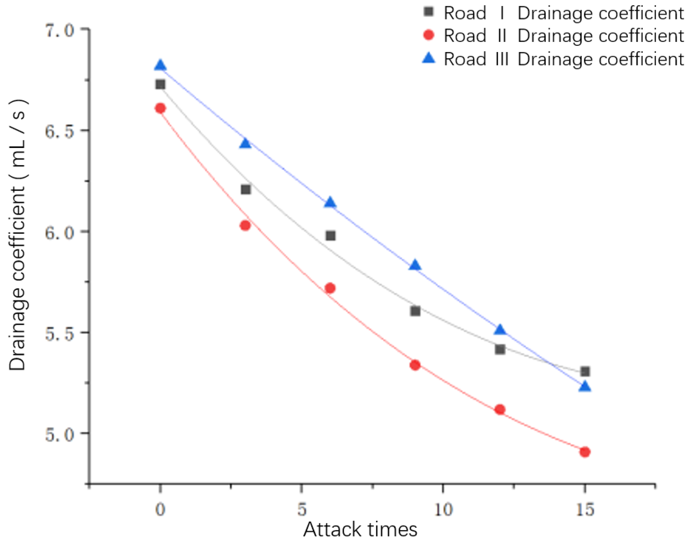
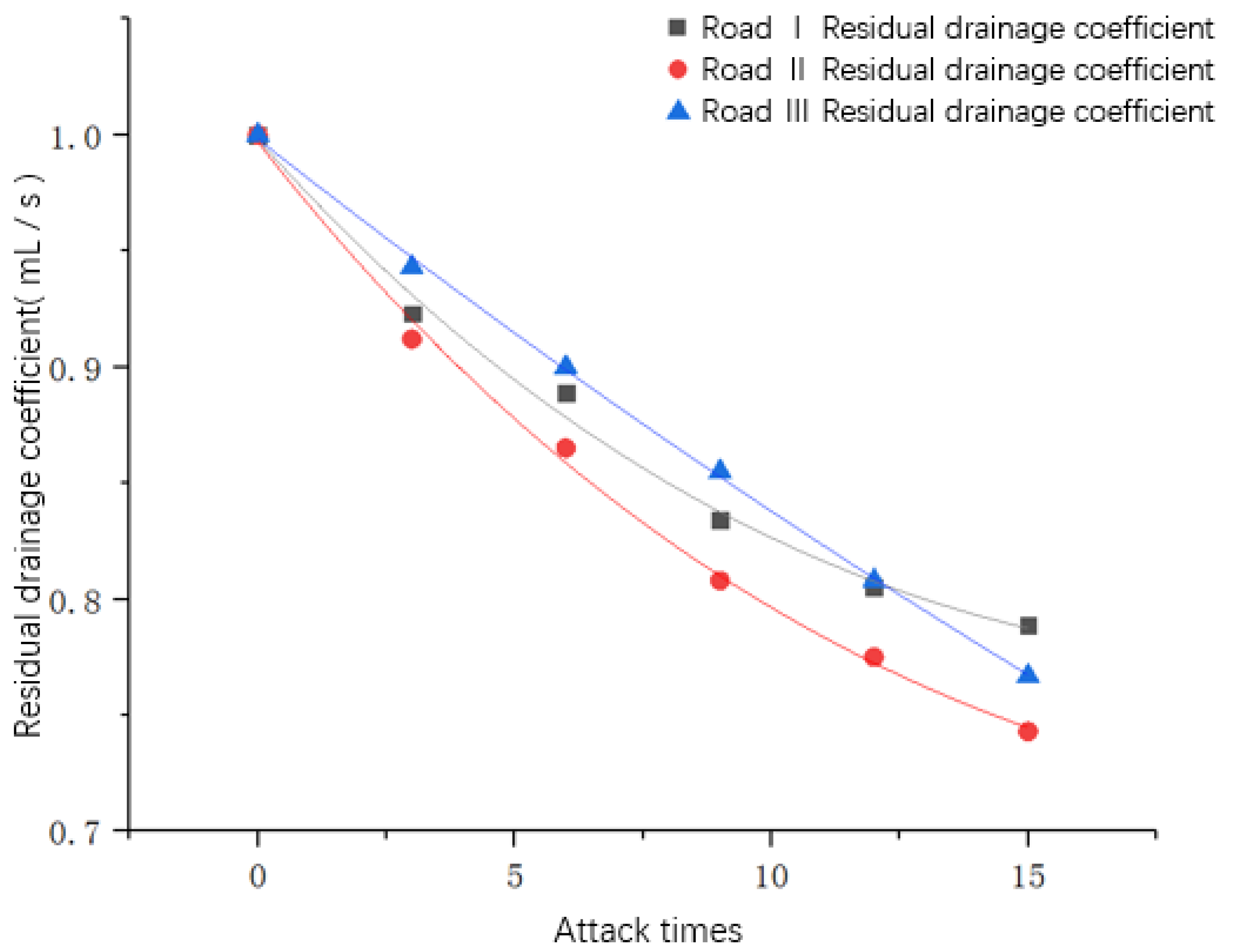
Assuming that Road I is blocked with 9 g of fine particles, it can be seen from Figure 3 that the water drainage coefficient decreases to 60% of its initial value. After nine compactions, it can be seen from Figure 5 that the drainage coefficient decreases to 80% of its initial value. This sharp reduction in the drainage coefficient provides a basis for determining the maintenance time.

The blocking quality and compaction times are incorporated into the decay size and velocity function of the drainage coefficient; the decision matrix of the three roads is summarized in

Table 11. Decision matrix of the environment and usage of the three roads.

Index Graduation	Blocking Instantaneous Velocity	Compaction Instantaneous Velocity	Decay of Drainage Coefficient Caused by Blockage	Decay of Drainage Coefficient Caused by Compaction	Ratio of Traffic Volume	Maximum Annual Rainfall in a Single Day in 5 Years	Wind Scale
Road I	0.18100	0.07841	2.27016	1.09456	58,691	239.5	3
Road Ⅱ	0.22400	0.07493	1.57645	1.47548	75,828	193.0	2
Road Ⅲ	0.13791	0.07618	2.59137	2.36666	157,421	140.9	4

.

We establish a data matrix as follows:

$$A=\left[\begin{array}{ccccccc}0.18100& 0.07841& 2.27016& 1.09456& 58691& 239.5& 3\\ 0.22400& 0.07493& 1.57645& 1.47548& 75828& 193.0& 2\\ 0.13791& 0.07618& 2.59137& 2.36666& 157421& 140.9& 4\end{array}\right]$$

(17)

According to Equation (8), the matrix $P$ is as follows:

$$P=\left[\begin{array}{ccccccc}0.333& 0.342& 0.353& 0.222& 0.201& 0.418& 0.333\\ 0.413& 0.326& 0.245& 0.299& 0.260& 0.336& 0.222\\ 0.254& 0.332& 0.402& 0.479& 0.539& 0.246& 0.445\end{array}\right]$$

(18)

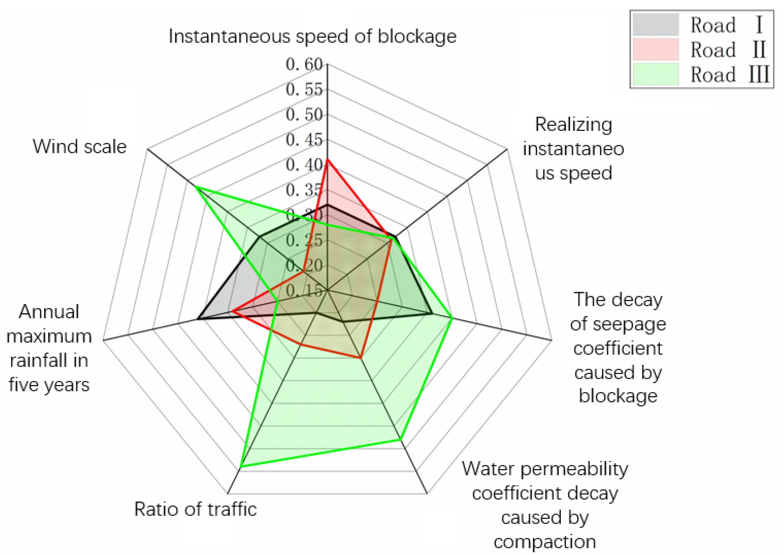
To clearly show the ratio of each index of the three roads, a radar map is drawn, as shown in Figure 7.

As shown in Figure 7, the influencing factors for Road III are highly dispersed, and the ratio of the traffic volume to the wind grade is the main influencing factor. The dispersion degree of the influencing factors for Roads I and II is low. For Road I, the maximum annual rainfall per day in five years is the main influencing factor, whereas for Road II, the instantaneous speed of blockage is the main influencing factor.

Using Equation (1), the following can be obtained:

$$E_j=\left[\begin{array}{ccc}0.9825& 0.9998& \begin{array}{ccc}0.9817& 0.9536& \begin{array}{ccc}0.9155& 0.9522& 0.9654\end{array}\end{array}\end{array}\right]$$

(19)

Because $D_j=1-E_j$,

$$D_j=\left[\begin{array}{ccc}0.0175& 0.0002& \begin{array}{ccc}0.0173& 0.0464& \begin{array}{ccc}0.0845& 0.0478& 0.0346\end{array}\end{array}\end{array}\right]$$

(20)

The first type of weights can be obtained from Equation (3), as follows:

$$W_j=\left[\begin{array}{ccc}0.0705& 0.0008& \begin{array}{ccc}0.0697& 0.1869& \begin{array}{ccc}0.3403& 0.1925& 0.1393\end{array}\end{array}\end{array}\right]$$

(21)

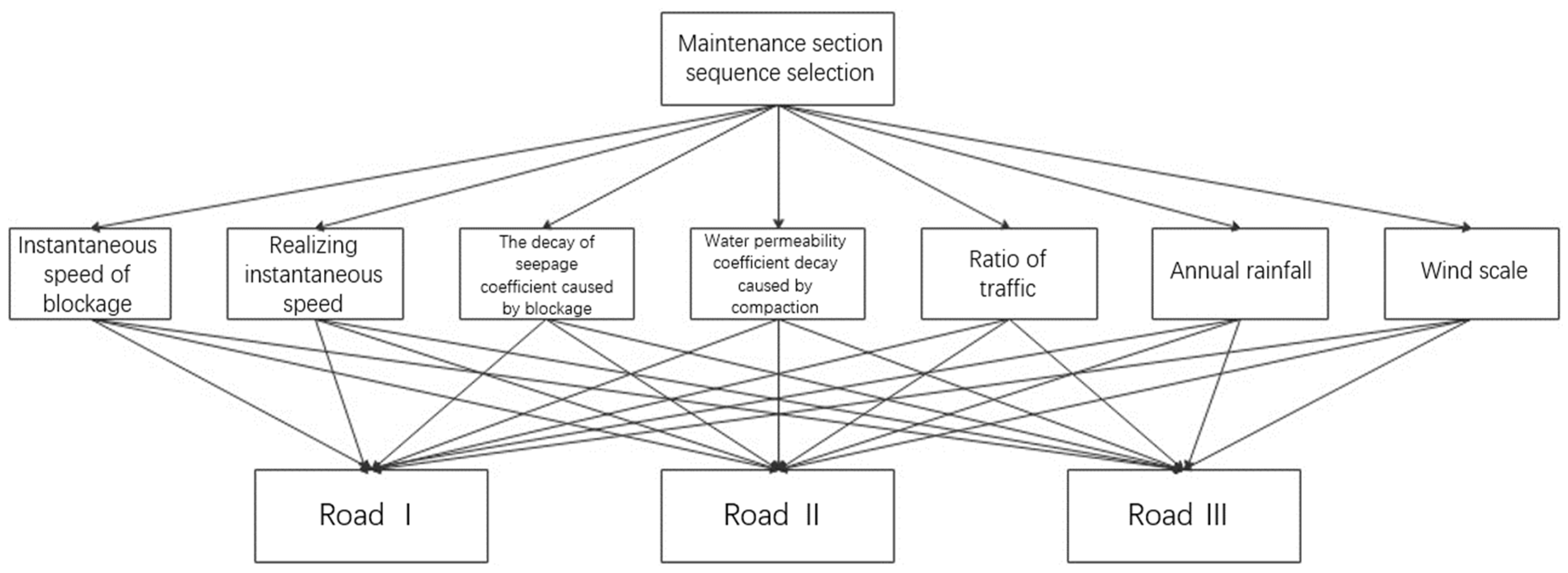
We establish the hierarchical model and draw the hierarchical structure diagram of the three roads, as shown in Figure 8.

According to the first type of weight, the matrix relationship between layers A and $Z$ is established. In the past 3 years, the average annual growth rate of the GDP in the three regions was 8.08%; thus, the traffic volume is bound to increase each year. A subjective adjustment was made to reduce the drainage coefficient attenuation. The adjusted weights $W_j$ were also subjectively adjusted. The reductions in instantaneous drainage speed, annual rainfall, and wind scale were due to the blockage of 8.08%. Meanwhile, it is increased to the ratio of drainage coefficient decay caused by compaction and that of instantaneous drainage velocity to traffic volume. The adjusted weights were as follows:

$$W_j=\left[\begin{array}{ccc}0.0648& 0.0065& \begin{array}{ccc}0.0641& 0.1925& \begin{array}{ccc}0.3672& 0.1769& 0.1280\end{array}\end{array}\end{array}\right]$$

(22)

$$B=\left[\begin{array}{ccccccc}1& 9.969& 0.011& 0.337& 0.176& 0.366& 0.506\\ 0.1& 1& 0.101& 0.034& 0.018& 0.037& 0.051\\ 0.989& 9.862& 1& 0.333& 0.175& 0.362& 0.501\\ 2.971& 29.615& 3.003& 1& 0.524& 1.088& 1.504\\ 5.667& 56.492& 5.729& 1.908& 1& 2.076& 2.869\\ 2.730& 27.215& 2.760& 0.919& 0.482& 1& 1.382\\ 1.975& 19.692& 1.997& 0.665& 0.349& 0.724& 1\end{array}\right]$$

(23)

The maximum characteristic root of matrix $B$ is 7.00107948. From Equations (6) and (7), it was found that $CI=0.000178$, $CR=0.000132<0.1$, the degree of inconsistency of the matrix is within the allowable range, and the $B$ normalized feature vector can be used as the weight vector.

The matrix of the sum of all the weights can be obtained using the summation method:

$$\left[\begin{array}{ccccccc}15.142& 153.845& 14.601& 5.196& 2.724& 5.653& 7.813\end{array}\right]$$

(24)

We calculate $P_{ij}=a_{ij}/{{\displaystyle \sum }}_{i=1}^n{a}_{ij}$, and a new matrix is obtained and summed horizontally. The results are summarized in

Table 12. Sub-indicators and summation.

$\mathit{Z}$	${\mathit{A}}_1$	${\mathit{A}}_2$	${\mathit{A}}_3$	${\mathit{A}}_4$	${\mathit{A}}_5$	${\mathit{A}}_6$	${\mathit{A}}_7$	Ʃ
$A_1$	0.06480	0.06480	0.00075	0.06486	0.06461	0.06474	0.06480	0.38932
$A_2$	0.00648	0.00650	0.00692	0.00654	0.00661	0.00655	0.00653	0.04613
$A_3$	0.06409	0.06410	0.06849	0.06409	0.06424	0.06404	0.06412	0.45317
$A_4$	0.19252	0.19250	0.20567	0.19246	0.19236	0.19246	0.19250	1.36047
$A_5$	0.36722	0.36720	0.39237	0.36721	0.36711	0.36724	0.36721	2.59556
$A_6$	0.17691	0.17690	0.18903	0.17687	0.17695	0.17690	0.17688	1.25044
$A_7$	0.12798	0.12780	0.13677	0.12798	0.12812	0.12807	0.12799	0.90471

.

From Table 12, the following equation is obtained:

$$T_i/{\displaystyle \sum }_{i=1}^n{T}_i=\left[\begin{array}{ccc}0.0566& 0.0066& \begin{array}{ccc}0.0647& 0.1944& \begin{array}{ccc}0.3708& 0.1786& 0.1292\end{array}\end{array}\end{array}\right]$$

(25)

The matrix relationship between levels $B$ and $A$ is established, and the previous steps are repeated to obtain the transpose matrix composed of eigenvalues and eigenvectors:

$${\mathsf{\lambda }}_{max}=\left[\begin{array}{ccc}3.0001& 2.9995& \begin{array}{ccc}3.0003& 3.0008& \begin{array}{ccc}3.0003& 2.9995& 2.9998\end{array}\end{array}\end{array}\right]$$

(26)

$$T=\left[\begin{array}{ccccccc}0.567& 0.591& 0.599& 0.365& 0.318& 0.504& 0.557\\ 0.702& 0.566& 0.416& 0.492& 0.411& 0.600& 0.372\\ 0.432& 0.574& 0.684& 0.790& 0.854& 0.622& 0.742\end{array}\right]$$

(27)

A consistency inspection indicates that $T$ meets the requirements.

The importance of schemes $B_1$–$B_3$ is as follows:

$$\left[\begin{array}{ccccccc}0.567& 0.591& 0.599& 0.365& 0.318& 0.504& 0.557\\ 0.702& 0.566& 0.416& 0.492& 0.411& 0.600& 0.372\\ 0.432& 0.574& 0.684& 0.790& 0.854& 0.622& 0.742\end{array}\right]·[\begin{array}{c}0.0556\\ 0.0066\\ 0.0647\\ 0.1944\\ 0.3708\\ 0.1756\\ 0.1292\end{array}]=\left[\begin{array}{c}0.4250\\ 0.4729\\ 0.7473\end{array}\right]$$

(28)

Moreover, $0.7473>0.4729>0.4250$. Thus, the maintenance urgency should be in the following order: Road III > Road II > Road I.

5.2. Determination of Maintenance Opportunity

The urgency of road maintenance determines the maintenance order [38]. However, we can ensure economic benefits and maintain sustainable development on the premise of maintaining the road service level by determining only the appropriate maintenance opportunity. Therefore, the specific maintenance opportunity was calculated.

Owing to the existence of the cross-slope of the road arch, the rainfall flows from the center to the inner edge the pavement [39]. Taking half of the road surface as the reference object, the width of the road surface is $L$, which is evenly divided into $k$ segments. The center of the pavement’s cross-section is the starting point of rainwater flow, and the edge is the end point; hence, the rainwater flows to section $k$, and the length of each section is $\frac{L}{k}$. If $k\to \infty$, then $\frac{L}{k}\to 0$.

When the rainfall speed is low and the transverse rainwater cannot be collected into the water flow, the quality of the first transmitted rainwater is as follows (assuming that after the rainfall, the rainfall quality per unit area is $q$, and the transmission efficiency is $\mathsf{\gamma }$):

$$m_1=\mathsf{\gamma }q\left(1-\mathsf{\gamma }\right)\frac{L}{k}=\mathsf{\gamma }\left(1-\mathsf{\gamma }\right)\frac{L}{k}q$$

(29)

The rainwater quality at each point was determined; the results are summarized in

Table 13. Calculation table of rainwater quality at each point.

First Point	Second Point	Third Point	……	$\mathbf{Sequence}\mathit{k}-1\mathbf{Point}$	$\mathbf{Sequence}\mathit{k}$
$\frac{\mathsf{\gamma }\left(1-\mathsf{\gamma }\right)qL}{k}$	$\frac{\mathsf{\gamma }{\left(1-\mathsf{\gamma }\right)}^{2}qL}{k}$	$\frac{\mathsf{\gamma }{\left(1-\mathsf{\gamma }\right)}^{3}qL}{k}$	……	$\frac{\mathsf{\gamma }{\left(1-\mathsf{\gamma }\right)}^{\left(k-1\right)}qL}{k}$	$\frac{\mathsf{\gamma }{\left(1-\mathsf{\gamma }\right)}^{k}qL}{k}$

.

$$\mathrm{Sumation}=S_k=\frac{Lq}{k}\left(1-\mathsf{\gamma }\right)\left[1-{\left(1-\mathsf{\gamma }\right)}^k\right]$$

(30)

The drainage quality per unit pavement area on rainy days can be obtained using Equation (27).

However, when the rainfall rate is high and the water storage capacity of the pavement is saturated, the rainwater stored per unit pavement length is closer to a fixed value $\mathsf{\eta }$, which is related to the internal spatial structure of the permeable asphalt pavement.

When measuring the drainage coefficient, the mass of the test piece before measurement is taken as $m_1$, and that after measurement is taken as $m_2$, owing to water infiltration. The water storage capacity of the test piece per unit length is $\mathsf{\eta }$, which is obtained as follows:

$$\mathsf{\eta }=16.7\left(m_2-m_1\right)$$

(31)

The mass of accumulated water in the pavement $m_{aw}$ is

$$m_{aw}=\mathsf{\eta }L$$

(32)

The drainage mass $m$ is

$$m=qL-\mathsf{\eta }L$$

(33)

Permeable asphalt mixtures have excellent drainage capacity; therefore, we only considered the pavement saturation state.

The test pieces were prepared according to the mix proportions of the three roads, and the drainage coefficient was measured accordingly. The $\eta$ values obtained from the three groups of test pieces are listed in

Table 14. $\mathsf{\eta }$ values of the three roads.

Type of Mixture	Road I	Road II	Road III
$\mathsf{\eta }$	15.1	13.7	16.7

.

Assuming that the three roads have six lanes and that half the width of the pavement is 11.25 m, the water storage capacity of the road is 11.25$\mathsf{\eta }$.

The meteorological department classifies rainfall as light rain, moderate rain, heavy rain, and rainstorms (

Table 15. Rainfall classification.

Rainfall Grade	Light Rain	Moderate Rain	Heavy Rain	Rainstorms
Rainfall (mm/h)	<1.5	1.6–6.9	7–14.9	15–40

) [40,41]. Therefore, the rainfall scale should be considered in the selection of maintenance opportunities. During light or moderate rain, a water-free film of permeable asphalt pavement is produced; however, the impact of rainfall was not considered in this study [42]. To ensure a more detailed distinction between the selection of maintenance opportunity, the rainstorm is classified into small and large rainstorms. The rainfall rates for heavy rain, small rainstorms, and large rainstorm are 15, 27.5, and 40 mm/h, respectively.

The mass of rainwater discharged from a half-width pavement with a length of 6 cm in 1 h is obtained as follows:

$$W_{DRA}=1\times 6\times 1125H_{PHR}-11.25\mathsf{\eta }=6750H_{PHR}-11.25\mathsf{\eta }$$

(34)

where $W_{DRA}$ denotes the mass of discharged rainwater, and $H_{PHR}$ is the rainfall per hour.

The road drainage mass is the difference between the total rainfall in 1 h and the water storage capacity, as summarized in

Table 16. Water storage capacity and drainage capacity of the three roads.

Road	Water Storage Capacity (mL)	Mass of Rainwater Discharged during Heavy Rain (mL)	Mass of Rainwater Discharged during Small Rainstorm (mL)	Mass of Rainwater Discharged during Large Rainstorm (mL)
Road I	2831.25	7743.75	12,806.25	17,868.75
Road Ⅱ	2568.75	7556.25	12,618.75	17,681.25
Road Ⅲ	3131.25	6993.75	12,056.25	17,118.75

.

From the mass of blocked particles and the compaction times of the three roads (Table 10), the residual rate of the drainage coefficient of the permeable asphalt mixture can be obtained by fitting the decline function of the drainage coefficient with the decline function of drainage speed.

The amount of discharged rainwater is replaced in Equation (11), and the blocked particle mass of the test piece is converted according to the top surface area of the test piece shown in Figure 2 to obtain the blocked mass per unit area when meeting different drainage requirements, as shown in

Table 17. Quality of blocked particles when maintenance is needed to meet drainage requirements.

Item	Heavy Rain	Small Rainstorm	Large Rainstorm
Road Ⅰ mass of blocking (g/m2)	5958.89	2755.78	1194.54
Road Ⅱ mass of blocking (g/m2)	5500.44	2111.28	872.29
Road Ⅲ mass of blocking (g/m2)	3936.43	1489.01	625.05

.

6. Conclusions

In this study, we proposed an advanced method to evaluate maintenance opportunities for permeable asphalt pavements based on an entropy–AHP analysis. The following are the main conclusions drawn in this study.

(1)

A combination of the entropy method and AHP, and that of subjective and objective assessments, were used for the weighting and selection of maintenance schemes; this addressed the problem of sequence selection for road maintenance.

(2)

The decrease in the mixture void ratio caused by blockage or compaction leads to a parabolic exponential decline in the drainage coefficient. The smaller the void ratio, the more difficult it is for the permeable pavement to be compressed, and the slower the decline of the drainage coefficient.

(3)

During service, the factors affecting the urgency of maintenance are the instantaneous rate of pavement blockage, instantaneous rate of compaction, decay of the water permeability coefficient caused by the blockage, decay of the water permeability coefficient caused by the compaction, traffic volume, rainfall, and wind scale.

(4)

The urgency of maintenance for the three typical test roads was determined using the entropy–AHP method: Road III > Road II > Road I. Thus, the proposed calculation model for road drainage capacity can accurately predict suitable opportunities for pavement maintenance.

References

1. Zhang, Z.W.; Sha, A.M.; Liu, X.; Luan, B.; Gao, J.; Jiang, W.; Ma, F. State-of-the-art of porous asphalt pavement: Experience and considerations of mixture design. Constr. Build. Mater. 2020, 262, 119998. [Google Scholar] [CrossRef]
2. Bilodeau, J.P.; Doré, G.; Savoie, C. Laboratory evaluation of flexible pavement structures containing geocomposite drainage layers using light weight deflectometer. Geotext. Geomembr. 2015, 43, 162–170. [Google Scholar] [CrossRef]
3. Zhang, M.; Guo, C.; Yu, B.; Yang, Y.; Lu, Z. CTCP temperature fields and stresses. Int. J. Pavement Res. Technol. 2017, 10, 553–562. [Google Scholar] [CrossRef]
4. Sañudo-Fontaneda, L.A.; Charlesworth, S.M.; Castro-Fresno, D.; Andrés-Valeri, V.C.; Rodríguez-Hernández, J. Water quality and quantity assessment of pervious pavements performance in experimental car park areas. Water Sci. Technol. 2014, 69 7, 1526–1533. [Google Scholar] [CrossRef]
5. Hernando, D.; Smith, R.T.; Sholar, G.A.; Choubane, B. Study of the field hydraulic conductivity of thin open-graded friction courses. Constr. Build. Mater. 2021, 299, 124236. [Google Scholar] [CrossRef]
6. Hernandez-Saenz, M.A.; Caro, S.; Arámbula-Mercado, E.; Martin, A.E. Mix design, performance and maintenance of permeable friction courses (PFC) in the United States: State of the art. Constr. Build. Mater. 2016, 111, 358–367. [Google Scholar] [CrossRef]
7. Kandhal, P.S.; Mallick, R.; Aschenbrener, T.; Adam, J.F.; Al-Qadi, I.L.; Brooker, A.C.; Brosseaud, Y.; Carpenter, S.H.; D’Angelo, J.A.; Huber, G.; et al. Open-Graded Friction Course: State of the Practice; E-C005; Technical Report for Transportation Research Board: Washington, DC, USA, December 1998. [Google Scholar]
8. Alvarez, A.E.; Martin, A.E.; Estakhri, C.K. A review of mix design and evaluation research for permeable friction course mixtures. Constr. Build. Mater 2011, 25, 1159–1166. [Google Scholar] [CrossRef]
9. Alvarez, A.E.; Martin, A.E.; Estakhri, C.K. Optimizing the design of permeable friction course mixtures. Transp. Res. Rec. 2011, 2209, 26–33. [Google Scholar] [CrossRef]
10. Mo, L.; Huurman, M.; Woldekidan, M.F.; Wu, S.; Molenaar, A.A. Investigation into material optimization and development for improved ravelling resistant porous asphalt concrete. Mater. Design 2010, 31, 3194–3206. [Google Scholar] [CrossRef]
11. Disfani, M.M.; Mohammadinia, A.; Narsilio, G.A.; Aye, L. Performance evaluation of semi-flexible permeable pavements under cyclic loads. Int. J. Pavement Eng. 2020, 21, 336–346. [Google Scholar] [CrossRef]
12. Yong, C.F.; Mccarthy, D.T.; Deletic, A. Predicting physical clogging of porous and permeable pavements. J. Hydrol. 2013, 481, 48–55. [Google Scholar] [CrossRef]
13. Chen, Y.; Tebaldi, G.; Roque, R.; Lopp, G.; Su, Y. Effects of interface condition characteristics on open-graded friction course top-down cracking performance. Road Mater. Pavement Des. 2012, 13, 56–75. [Google Scholar] [CrossRef]
14. Kamiya, K.; Kazato, T. A study on repair design method of porous asphalt for the japanese motorways. Int. Conf. Transp. Geotech. 2012, 854–859. [Google Scholar]
15. Tan, S.; Fwa, T.F.; Guwe, V.Y. Laboratory measurements and analysis of clogging mechanism of porous asphalt mixes. J. Test. Eval. 2000, 28, 207–216. [Google Scholar]
16. Gonzzalez-Angullo, N.; Castro, D.; Rodríguez-Hernández, J.; Davies, J.W. Runoff infiltration to permeable paving in clogged conditions. Urban Water J. 2008, 5, 117–124. [Google Scholar] [CrossRef]
17. Coleri, E.; Kayhanian, M.; Harvey, J.T.; Yang, K.H.; Boone, J.M. Clogging evaluation of open graded friction course pavement tested under rainfall and heavy vehicle simulators. J. Environ. Eng. 2013, 129, 164–172. [Google Scholar] [CrossRef]
18. Moriyoshi, A.; Jin, T.; Nakai, T.; Ishikawa, H. Evaluation methods for porous asphalt pavement in service for fourteen years. Constr. Build. Mater. 2013, 42, 190–195. [Google Scholar] [CrossRef] [Green Version]
19. Tang, P.Z.; Chen, D.; Hou, Y.S. Entropy method combined with extreme learning machine method for the short-term photovoltaic power generation forecasting. Chaos Soliton Fract. 2016, 89, 243–248. [Google Scholar] [CrossRef]
20. Zhang, L.; Wu, K.X.; Liu, Y. Investigation on multi-objective performance optimization algorithm application of fan based on response surface method and entropy method. J. Therm. Sci. 2017, 26, 533–539. [Google Scholar] [CrossRef]
21. Liu, Y.; Eckert, C.M.; Earl, C.F. A review of fuzzy AHP methods for decision-making with subjective judgements. Expert Syst. Appl. 2020, 161, 113738. [Google Scholar] [CrossRef]
22. Yilmaz, F.C.; Zengin, M.; Cure, C.T. Determination of ecologically sensitive areas in Denizli province using geographic information systems (GIS) and analytical hierarchy process (AHP). Environ. Monit. Assess. 2020, 192, 1–3. [Google Scholar] [CrossRef]
23. Ozkul, S.D.; Harmancioglu, N.B.; Singh, V.P. Entropy-based assessment of water quality monitoring networks. J. Hydrol. Eng. 2000, 5, 90–100. [Google Scholar] [CrossRef] [Green Version]
24. Pérez-Acebo, H.; Linares-Unamunzaga, A.; Rojí, E.; Gonzalo-Orden, H. IRI performance models for flexible pavements in two-lane roads until first maintenance and/or rehabilitation work. Coatings 2020, 10, 97. [Google Scholar] [CrossRef] [Green Version]
25. Saaty, T.L. A scaling method for priorities in hierarchical structures. J. Math. Psychol. 1997, 15, 234–281. [Google Scholar] [CrossRef]
26. Tashman, L.; Wang, L.; Thyagarajan, S. Microstructure characterization for modeling hma behavior using imaging technology. Road Mater. Pavement Des. 2007, 8, 207–238. [Google Scholar] [CrossRef]
27. Shirini, B.; Imaninasab, R. Performance evaluation of rubberized and SBS modified porous asphalt mixtures. Constr. Build. Mater. 2016, 107, 165–171. [Google Scholar] [CrossRef]
28. CJJ/T90. Technical Specification for Permeable Asphalt Pavement; Profession Standard of the People’s Republic of China: Beijing, China, 2012.
29. Martin, W.D.; Putman, B.J.; Neptune, A.I. Influence of aggregate gradation on clogging characteristics of porous asphalt mixtures. J. Mater. Civ. Eng. 2014, 26, 04014026. [Google Scholar] [CrossRef]
30. Suresha, S.N.; Varghese, G.; Shankar, A.U. Laboratory and theoretical evaluation of clogging behaviour of porous friction course mixes. Int. J. Pavement Eng. 2010, 11, 61–70. [Google Scholar] [CrossRef]
31. Wang, T.D.; Hu, L.Q.; Pan, X.D.; Xu, S.; Yun, D. Effect of the compactness on the texture and friction of asphalt concrete intended for wearing course of the road pavement. Coatings 2020, 10, 192. [Google Scholar] [CrossRef] [Green Version]
32. You, Z.Y.; Adhikari, S.; Emin, K.M. Dynamic modulus simulation of the asphalt concrete using the x-ray computed tomography images. Mater. Struct. 2009, 42, 617–630. [Google Scholar] [CrossRef]
33. Chaturabong, P. Evaluation of bleeding resistance in chip seal and asphalt emulsion residue rheology. Coatings 2019, 9, 670. [Google Scholar] [CrossRef] [Green Version]
34. Safoura, S.; Mehrdad, A.; Jayantha, K.; Ross, G. Sustainable pavement construction: A systematic literature review of environmental and economic analysis of recycled materials. J. Clean. Prod. 2021, 313, 127936. [Google Scholar]
35. Wang, Y.; Chen, X.; Han, Y.; Guo, S. Forecast of passenger and freight traffic volume based on elasticity coefficient method and grey model. Procedia Soc. Behav. Sci. 2013, 96, 136–147. [Google Scholar] [CrossRef] [Green Version]
36. Hengl, H.L.; Füssl, J. The influence of superelevated profiles of paving block structures on their load-bearing behavior. Eng. Struct. 2016, 117, 195–203. [Google Scholar] [CrossRef]
37. Xie, S.; Qu, J.; Han, Q.; Pang, Y. Wind dynamic environment and wind tunnel simulation experiment of bridge sand damage in Xierong section of Lhasa–Linzhi railway. Sustainability 2020, 12, 5689. [Google Scholar] [CrossRef]
38. Bo, L.; Kundwa, M.J.; Jiao, C.Y.; Wei, Z.X. Pavement performance evaluation and maintenance decision-making in Rwanda. Int. J. Pavement Res. Technol. 2019, 12, 443–447. [Google Scholar] [CrossRef]
39. Luo, W.T.; Li, L.; Wang, K.C.; Wei, C.C. Surface drainage evaluation of asphalt pavement using a new analytical water film depth model. Road Mater. Pavement Des. 2020, 21, 1985–2004. [Google Scholar] [CrossRef]
40. Yang, Q.X.; Beecham, S.; Liu, J.X.; Pezzaniti, D. The influence of rainfall intensity and duration on sediment pathways and subsequent clogging in permeable pavements. J. Environ. Manag. 2019, 246, 730–736. [Google Scholar] [CrossRef]
41. GB/T 28592-2012. Grade of Precipitation; National Standardization Administration Committee: Beijing, China, 2012.
42. Hou, J.M.; Zhang, Y.W.; Tong, Y.; Guo, K.H.; Qi, W.C.; Hinkelmann, R. experimental study for effects of terrain features and rainfall intensity on infiltration rate of modelled permeable pavement. J. Environ. Manag. 2019, 243, 177–186. [Google Scholar] [CrossRef]
Figure 1. Hierarchical structure diagram.
Coatings 11 01516 g001
Figure 2. Test piece for permeability coefficient test: (a) test piece after cutting; (b) coated epoxy resin on the cubic specimen.
Coatings 11 01516 g002
Figure 3. Relationship between the drainage coefficient and blocked particle mass.
Coatings 11 01516 g003
Figure 4. Relationship between the residual rate of drainage coefficient and blocked particle mass.
Coatings 11 01516 g004
Figure 5. Relationship between the drainage coefficient and compaction times.
Coatings 11 01516 g005
Figure 6. Relationship between the residual rate of drainage coefficient and compaction times.
Coatings 11 01516 g006
Figure 7. Ratio of the indexes of the three roads.
Coatings 11 01516 g007
Figure 8. Hierarchical structure diagram of the three roads.
Coatings 11 01516 g008