Mathematical Analysis of Entropy Generation in the Flow of Viscoelastic Nanofluid through an Annular Region of Two Asymmetric Annuli Having Flexible Surfaces

Abstract

In this manuscript, the authors developed the mathematical model for entropy generation analysis during the peristaltic propulsion of Jeffrey nanofluids passing in a midst of two eccentric asymmetric annuli. The model was structured by implementation of lubrication perspective and dimensionless strategy. Entropy generation caused by the irreversible influence of heat and mass transfer of nanofluid and viscous dissipation of the considered liquid was taken into consideration. The governing equations were handled by a powerful analytical technique (HPM). The comparison of total entropy with the partial entropy was also invoked by discussing Bejan number results. The influence of various associated variables on the profiles of velocity, temperature, nanoparticle concentration, entropy generation and Bejan number was formulated by portraying the figures. Mainly from graphical observations, we analyzed that, in the matter of thermophoresis parameter and Brownian motion parameter, entropy generation is thoroughly enhanced while inverse readings were reported for the temperature difference parameter and the ratio of temperature to concentration parameters.

1. Introduction

Nanofluid, characterized by a significant increase in a number of properties compared to conventional engineered fluid [1], is found to serve in many practical applications, for example, petroleum engineering [2,3,4,5], power industry [6,7], and medical science [8,9], which has drawn particular attentions for cancer treatments in recent years. Cancer covers a huge group of diseases which can damage any portion of the body. Nowadays, cancer is a main cause of death all over the world, around 70% of cancer deaths materialize in middle- and low-income countries. There are many treatments to cure cancer, such as surgery, radiation and chemotherapy, but these procedures may harm the normal tissue. Hanahan and Weinberg [10] have explained six cancer hallmarks, helping to differentiate features between the tumor and normal tissue, and maybe come up with better alternative therapies. These hallmarks include inducing activating invasion and metastasis, resisting cell death, angiogenesis, enabling replicative immortality, sustaining proliferative signaling, and evading growth suppressors. Based on these cancer hallmarks, latest therapies for cancer treatment have been introduced. Nowadays, nanomedicine (nanomedicine is a branch of nanotechnology, or utilization of materials less than 100 nm, applied to medicine and health sciences) is the prominent procedure for treating cancer. The nanocarriers’ properties, including their targeting modifications, favorable drug release profiles, high surface-to-volume ratios, and nanoscale sizes, may authorize them to reach and target the tissue of a tumor and the deliverance of drugs in a stable and controlled manner. For cancer research, nanomaterials are available in modified shape, because to treat specific tumors, size and surface features are crucial. The size of the nanoparticle is a key attribute, which travel across the bloodstream, ensuring delivery of nanocarriers to tumor tissue. The small-scale nanoparticles can stockpile comfortably in the physiological tumor vessels and also extravagate into normal tissue. In view of many nanoparticle applications in bio-fluid flows, many researchers have concentrated their work in the field of bio-nanofluids. For instance, Prakash et al. [11] have presented the study of nanofluids which is relevant to bio-inspired nanofluid smart pump designs, which may also be exploited in smart-drug delivery. Abbas et al. [12] have provided mathematical modelling to describe the peristaltic transport of blood (blood is treated as nanofluid) and analyzed the entropy analysis. They concluded that such a study can help in analyzing blood flow in small blood vessels with elastic walls. Abdelsalam and Bhatti [13] have given a theoretical model to describe the effect of sundry variables on the feature of blood flows in the presence of nanoparticles, and suggested that Brownian motion and chemical reaction exhibit dual variation of nanoparticles’ volume fraction. Shah et al. [14] have presented the theoretical study, which is applicable to the drug-delivery system, as the micro-polar nanoparticles of gold are proficient drug-delivery and drug-carrying mediums. Bhatti et al. [15] studied the two-phase flow under the effects of coagulation with peristaltic pumping through the Prandtl stress model, with magnetic field and porous medium terms. They analyzed that friction forces flourish with the altitude of clot height and particle concentration, on the other hand they are minimized with other involving factors in the problem.

It is extensively known that biological liquids, such as gastric fluids and blood, generally behave as non-Newtonian fluids. Many researchers have considered Jeffrey/viscoelastic fluid as biological (synovial, blood, gastric, chyme, and saliva) fluid. To delineate the stress relaxation effects of real fluids, the viscoelastic fluid model is appropriately competent. These effects cannot describe the usual Newtonian fluid model. In addition to this, the Jeffrey fluid model can also describe the characteristic of memory-time scale. Kahshan et al. [16] have described the Creeping flow of a viscoelastic fluid in a channel with an application to flow in a flat-plate hemodialyzer. Pandey and Tripathi [17] have explored the viscoelastic fluid flow by peristalsis in a channel in order to apply the model to the swallowing of food-bolus through the esophagus. Ellahi et al. [18] used Jeffrey fluid as bio-fluid and studied the problem of the peristaltic flow of Jeffrey fluid in a non-uniform rectangular duct, which may be applicable to modern drug delivery systems with great utility. Ramesh et al. [19] have considered Jeffery’s viscoelastic formulation, which is employed in the rheology of blood. Some more studies can be seen through [20,21,22,23,24,25].

In thermodynamics, entropy is a measure of the number of specific modes in which a thermodynamic system can be organized, often called a measure of impedance or a measure of progress toward thermodynamic equilibrium. Pakdemirli and Yilbas [26] have analyzed the entropy generation mechanism of non-Newtonian fluid through a pipe. According to them, the entropy Brinkman number causes an increase in entropy generation. Entropy generation in a peristaltic pumping problem has been presented by Souidi et al. [27]. Heat and fluid flow causing entropy generation in backward-facing step flow is suggested by Abu-Nada [28]. More studies on entropy generation in peristaltic transports are reported in [29,30,31], but none of these established the entropy analysis of viscoelastic nanofluids in eccentric cylinders having a peristaltic outer surface.

Keeping in mind the physiological applications of a peristaltic propulsion of viscoelastic fluids, the investigators focused on the entropy generation and Bejan number during the peristaltic transport of viscoelastic nanofluid in the annulus region of two eccentric cylinders. The equations of governing the flow are considered in the cylindrical geometry. The concerned non-dimensional system of equations is solved using optimal homotropy perturbation technique under the long wavelength and low Reynolds number assumptions. The effects of involved parameters on the pressure rise, velocity, temperature, nanoparticle concentration, entropy generation, and Bejan number are shown through graphical illustrations.

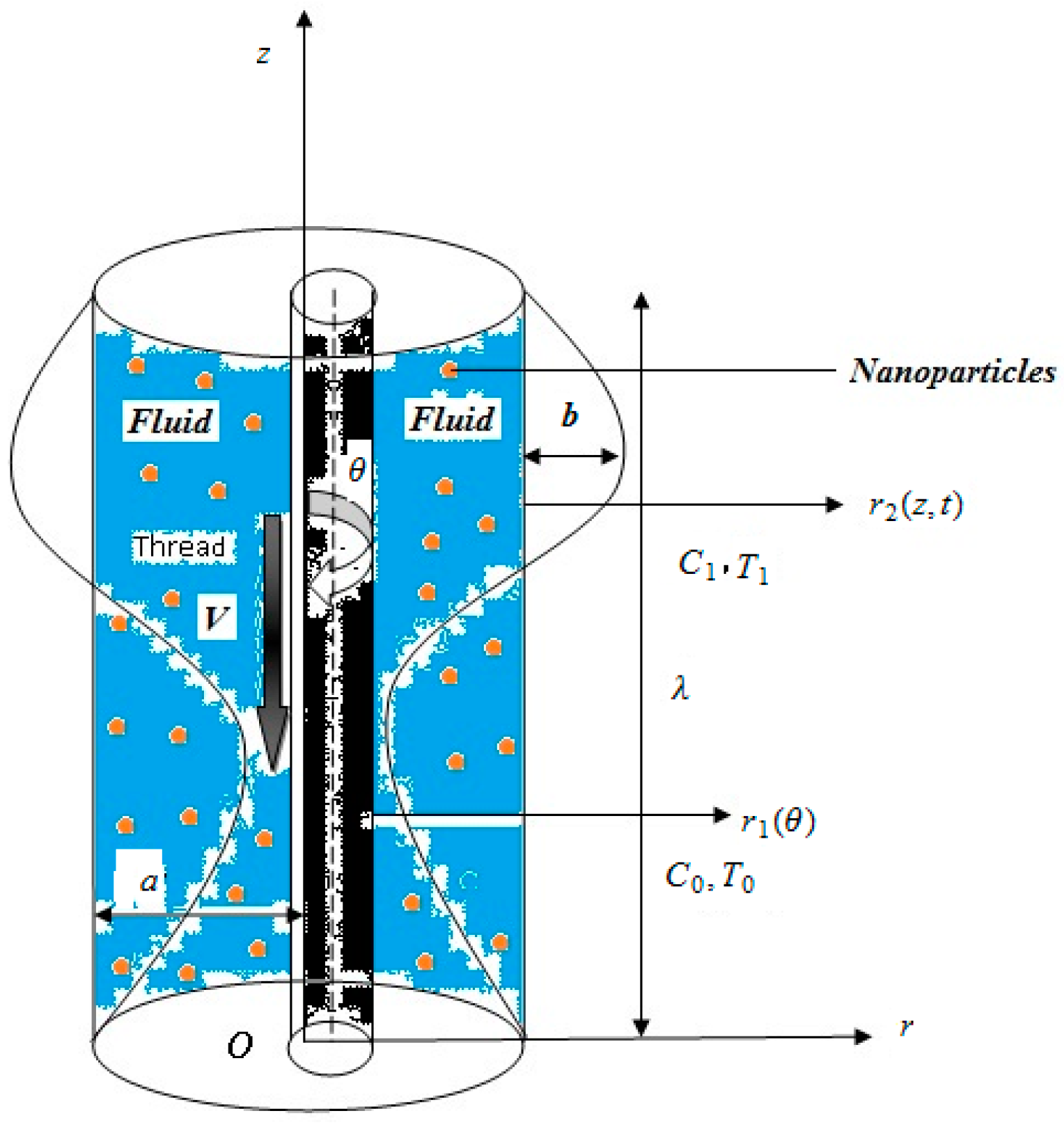
2. Mathematical Analysis

Let us analyze the entropy generation in three-dimensional flow of nanofluid with the Jeffrey model by considering the passage in a space between two eccentric annuli, with flexible outer surface along with inner rigid cylinder, going with the fluid with constant speed V. The walls of the outer annulus produce peristaltic waves along its length, which helps in pushing the fluid forward. A concentration $C_0$ of nanoparticles is assumed at the inner boundary, while the outer is maintained at $C_1$. The temperature distributions are described as $T_0$ and $T_1$ on the considered inner and lower walls accordingly (see Figure 1).

The physical behavior of inner and outer layers of the annuli is manipulated mathematically as follows:

${\chi }_i={\chi }_j+{\chi }_k\cos \gamma ,$ for $i=1,2$…, where ${\chi }_1$, ${\chi }_j=\delta$, ${\chi }_k=\epsilon ,$ and $\gamma =\theta$ are representing the inner cylinder walls. Similarly, ${\chi }_2$, ${\chi }_j=a$, ${\chi }_k=b,$ and $\gamma =\frac{2\pi }{\lambda }\left(z-ct\right)$ are suggesting the same for outer annuli. Above appearing $\delta , a, b, \lambda ,$ and $c$ are denoting the radii of inner and outer cylinders, the amplitude of the wave, the wavelength and the wave speed, orderly.

According to the considered geometry, the velocity components are suggested as $\left[w_1\left(r,\theta ,z\right),0,w_2\left(r,\theta ,z\right)\right]$. The mathematical structure of the given problem can be entertained by the following expressions based on physical laws:

$$\frac{\partial w_1}{\partial r}+\frac{\partial w_2}{\partial z}+\frac{w_1}{r}=0,\hspace{0.17em}$$

(1)

$${\rho }_f\left(\frac{\partial w_1}{\partial t}+w_1\frac{\partial w_1}{\partial r}+w_2\frac{\partial w_1}{\partial z}\right)=-\frac{\partial p}{\partial r}+\frac{\partial {\Upsilon }_{11}}{\partial r}+\frac{1}{r}\frac{\partial {\Upsilon }_{12}}{\partial \theta }+\frac{\partial {\Upsilon }_{13}}{\partial z}+\frac{{\Upsilon }_{11}}{r}-\frac{{\Upsilon }_{22}}{r},\hspace{0.17em}$$

(2)

$$0=-\frac{1}{r}\frac{\partial p}{\partial \theta }+\frac{\partial {\Upsilon }_{12}}{\partial r}+\frac{1}{r}\frac{\partial {\Upsilon }_{22}}{\partial \theta }+\frac{\partial {\Upsilon }_{23}}{\partial z}+\frac{{\Upsilon }_{21}}{r}+\frac{{\Upsilon }_{12}}{r},\hspace{0.17em}$$

(3)

$$\begin{array}{c}\begin{array}{r}{\rho }_f\left(\frac{\partial w_2}{\partial t}+w_1\frac{\partial w_2}{\partial r}+w_2\frac{\partial w_2}{\partial z}\right)=-\frac{\partial p}{\partial z}+\frac{\partial {\Upsilon }_{31}}{\partial r}+\frac{1}{r}\frac{\partial {\Upsilon }_{32}}{\partial \theta }+\frac{\partial {\Upsilon }_{33}}{\partial z}+\frac{{\Upsilon }_{31}}{r}\\ \hspace{0.17em}\hspace{0.17em}\hspace{0.17em}\hspace{0.17em}\hspace{0.17em}\hspace{0.17em}\hspace{0.17em}\hspace{0.17em}\hspace{0.17em}\hspace{0.17em}\hspace{0.17em}\hspace{0.17em}\hspace{0.17em}\hspace{0.17em}\hspace{0.17em}\hspace{0.17em}\hspace{0.17em}\hspace{0.17em}\hspace{0.17em}\hspace{0.17em}\hspace{0.17em}\hspace{0.17em}\hspace{0.17em}\hspace{0.17em}\hspace{0.17em}\hspace{0.17em}\hspace{0.17em}\hspace{0.17em}\hspace{0.17em}\hspace{0.17em}\hspace{0.17em}\hspace{0.17em}\hspace{0.17em}\hspace{0.17em}\hspace{0.17em}\hspace{0.17em}\hspace{0.17em}\hspace{0.17em}\hspace{0.17em}\hspace{0.17em}\hspace{0.17em}\hspace{0.17em}\hspace{0.17em}\hspace{0.17em}\hspace{0.17em}\hspace{0.17em}\hspace{0.17em}\hspace{0.17em}\hspace{0.17em}\hspace{0.17em}\hspace{0.17em}\hspace{0.17em}\hspace{0.17em}\hspace{0.17em}\hspace{0.17em}\hspace{0.17em}\hspace{0.17em}\hspace{0.17em}\hspace{0.17em}\hspace{0.17em}\hspace{0.17em}\hspace{0.17em}\hspace{0.17em}\hspace{0.17em}+{\rho }_{f}g\alpha \left(T-T_o\right)+{\rho }_{f}g\alpha \left(C-C_o\right),\end{array})\hspace{0.17em}\\ \hspace{0.17em}\end{array}$$

(4)

$$\begin{array}{c}\begin{array}{c}{\left(\rho c\right)}_f\left(\frac{\partial T}{\partial t}+w_1\frac{\partial T}{\partial r}+w_2\frac{\partial T}{\partial z}\right)=k\left(\frac{{\partial }^{2}T}{\partial r^2}+\frac{1}{r^2}\frac{{\partial }^{2}T}{\partial {\theta }^2}+\frac{{\partial }^{2}T}{\partial z^2}+\frac{1}{r}\frac{\partial T}{\partial r}\right)+{\left(\rho c\right)}_p\\ [D_B(\frac{\partial C}{\partial r}\frac{\partial T}{\partial r}+\frac{1}{r^2}\frac{\partial C}{\partial \theta }\frac{\partial T}{\partial \theta }+\frac{\partial C}{\partial z}\frac{\partial T}{\partial z})+\frac{D_T}{T_o}\left({\left(\frac{\partial T}{\partial r}\right)}^2+\frac{1}{r^2}{\left(\frac{\partial T}{\partial \theta }\right)}^2+{\left(\frac{\partial T}{\partial z}\right)}^2\right)]\\ +{\Upsilon }_{11}\frac{\partial w_1}{\partial r}+\frac{1}{r}{\Upsilon }_{12}\frac{\partial w_1}{\partial \theta }+{\Upsilon }_{13}\left(\frac{\partial w_1}{\partial z}+\frac{\partial w_2}{\partial r}\right)+\frac{1}{r}{\Upsilon }_{32}\frac{\partial w_2}{\partial \theta }+{\Upsilon }_{33}\frac{\partial w_2}{\partial z}+\frac{w_1}{r}{\Upsilon }_{22},\end{array})\hspace{0.17em}\\ \hspace{0.17em}\end{array}$$

(5)

$$\frac{\partial C}{\partial t}+w_1\frac{\partial C}{\partial r}+w_2\frac{\partial C}{\partial z}=D_B\left(\frac{{\partial }^{2}C}{\partial r^2}+\frac{1}{r^2}\frac{{\partial }^{2}C}{\partial {\theta }^2}+\frac{{\partial }^{2}C}{\partial z^2}+\frac{1}{r}\frac{\partial C}{\partial r}\right)+\frac{D_T}{T_o}\left(\frac{{\partial }^{2}T}{\partial r^2}+\frac{1}{r^2}\frac{{\partial }^{2}T}{\partial {\theta }^2}+\frac{{\partial }^{2}T}{\partial z^2}+\frac{1}{r}\frac{\partial T}{\partial r}\right).$$

(6)

In this study, constitutive relation used for fluid is the Jeffrey mode [18], which has the following expression:

$${\rm Y}=\frac{\mu }{1+{\lambda }_1}\left(\dot{\gamma }+{\lambda }_2\ddot{\gamma }\right).$$

(7)

To execute the collective effects of emerging parameters, we adopt the process of non-dimensionalization by introducing the following transformations [15,20,21,22,23,24]:

$$\begin{array}{l}p\prime =\frac{a^2}{\mu c\lambda }p,\hspace{0.17em}w\prime =\frac{w_2}{c},\hspace{0.17em}u\prime =\frac{\lambda }{ac}{w}_1,\hspace{0.17em}V\prime =\frac{V}{c},\hspace{0.17em}z\prime =\frac{z}{\lambda },\hspace{0.17em}r\prime =\frac{r}{a},\hspace{0.17em}\theta \prime =\theta ,\\ t\prime =\frac{c}{\lambda }t,\hspace{0.17em}\phi =\frac{b}{a},\hspace{0.17em}\epsilon \prime =\frac{\epsilon }{a},\hspace{0.17em}Re=\frac{\rho ca}{\mu },\hspace{0.17em}\delta \prime =\frac{\delta }{a},\hspace{0.17em}\overline{\theta }=\frac{T-T_o}{T_1-T_o},\\ {\delta }_o=\frac{a}{\lambda },\hspace{0.17em}\sigma =\frac{C-C_o}{\left(C_1-C_o\right)},\hspace{0.17em}{P}_r=\frac{\mu }{\rho \alpha },\hspace{0.17em}{S}_c=\frac{\mu }{\rho D_B},\hspace{0.17em}Br=\frac{{\rho }_{f}g\alpha a^2}{\mu c}\left(T_1-T_o\right),\\ Gr=\frac{{\rho }_{f}g\alpha a^2}{\mu c}\left(C_1-C_o\right),\hspace{0.17em}Nb=\frac{\tau D_B}{{\alpha }_f}\left(C_1-C_o\right),\hspace{0.17em}Nt=\frac{\tau D_T}{T_o{\alpha }_f}\left(T_1-T_o\right),\\ {\alpha }_f=\frac{k}{{\left(\rho c\right)}_f},\hspace{0.17em}\tau =\frac{{\left(\rho c\right)}_p}{{\left(\rho c\right)}_f},\hspace{0.17em}Gc=\frac{\mu c^2}{K\left(T_1-T_o\right)},S\prime =\frac{\mu c}{a}\Upsilon .\end{array})$$

In light of the above manufactured relations, the Equations (1) to (6) become

$$\frac{\partial u\prime }{\partial r\prime }+\frac{\partial w\prime }{\partial z\prime }+\frac{u\prime }{r\prime }=0,\hspace{0.17em}$$

(8)

$$\mathrm{Re}{\delta }_o\left(\frac{\partial u^{\prime }}{\partial t\prime }+u^{\prime }\frac{\partial w\prime }{\partial r\prime }+w\prime \frac{\partial u^{\prime }}{\partial z\prime }\right)=-\frac{\partial p\prime }{\partial r\prime }+{\delta }_o\frac{\partial S{\prime }_{11}^{}}{\partial r\prime }+{\delta }_o\frac{1}{r\prime }\frac{\partial S{\prime }_{12}^{{}^{}}}{\partial \theta \prime }+{\delta }_o^2\frac{\partial S{\prime }_{13}^{}}{\partial z\prime }+{\delta }_o\frac{S{\prime }_{11}^{}}{r\prime }-{\delta }_o\frac{S{\prime }_{22}^{{}^{}}}{r\prime }\hspace{0.17em},$$

(9)

$$0=-\frac{1}{r\prime }\frac{\partial p\prime }{\partial \theta \prime }+{\delta }_o\frac{\partial S{\prime }_{21}^{{}^{}}}{\partial r\prime }+{\delta }_o\frac{1}{r\prime }\frac{\partial S{\prime }_{22}^{}}{\partial \theta \prime }+{\delta }_o^2\frac{\partial S{\prime }_{23}^{}}{\partial z\prime }+{\delta }_o\frac{S{\prime }_{21}^{{}^{}}}{r\prime }+{\delta }_o\frac{S{\prime }_{12}^{{}^{}}}{r\prime },$$

(10)

$$\mathrm{Re}{\delta }_o\left(\frac{\partial w^{\prime }}{\partial t\prime }+u^{\prime }\frac{\partial w\prime }{\partial r\prime }+w\prime \frac{\partial w^{\prime }}{\partial z\prime }\right)=-\frac{\partial p\prime }{\partial z\prime }+\frac{\partial S{\prime }_{31}^{}}{\partial r\prime }+\frac{1}{r\prime }\frac{\partial S{\prime }_{32}^{}}{\partial \theta \prime }+{\delta }_o\frac{\partial S{\prime }_{33}^{}}{\partial z\prime }+\frac{S{\prime }_{31}^{{}^{}}}{r\prime }+Gr\overline{\theta }+Br\sigma ,$$

(11)

$$\begin{array}{l}{\delta }_o\mathrm{Re}{P}_r\left(\frac{\partial \overline{\theta }}{\partial T\prime }+u^{\prime }\frac{\partial \overline{\theta }}{\partial r\prime }+w\prime \frac{\partial \overline{\theta }}{\partial z\prime }\right)=\left(\frac{{\partial }^2\overline{\theta }}{\partial r{\prime }^2}+\frac{1}{r{\prime }^2}\frac{{\partial }^2\overline{\theta }}{\partial \theta {\prime }^2}+{\delta }_o^2\frac{{\partial }^2\overline{\theta }}{\partial z{\prime }^2}+\frac{1}{r\prime }\frac{\partial \overline{\theta }}{\partial r\prime }\right)\hspace{0.17em}\\ +Nb(\frac{\partial \sigma }{\partial r\prime }\frac{\partial \overline{\theta }}{\partial r\prime }+\frac{1}{r{\prime }^2}\frac{\partial \sigma }{\partial \theta \prime }\frac{\partial \overline{\theta }}{\partial \theta \prime }+{\delta }_o^2\frac{\partial \sigma }{\partial z\prime }\frac{\partial \overline{\theta }}{\partial z\prime })+Nt({\left(\frac{\partial \overline{\theta }}{\partial r\prime }\right)}^2+\frac{1}{r{\prime }^2}{\left(\frac{\partial \overline{\theta }}{\partial \theta \prime }\right)}^2\hspace{0.17em}\\ +{\delta }_o^2{\left(\frac{\partial \overline{\theta }}{\partial z\prime }\right)}^2)+Gc({\delta }_{o}S{\prime }_{11}^{{}^{}}\frac{\partial u\prime }{\partial r\prime }+{\delta }_o\frac{1}{r\prime }S{\prime }_{12}^{{}^{}}\frac{\partial u\prime }{\partial \theta \prime }+S{\prime }_{13}^{}\left({\delta }_o^2\frac{\partial u\prime }{\partial z\prime }+\frac{\partial w\prime }{\partial r\prime }\right)\hspace{0.17em}\\ +\frac{1}{r\prime }S{\prime }_{32}^{{}^{}}\frac{\partial w\prime }{\partial \theta \prime }+{\delta }_{o}S{\prime }_{33}^{}\frac{\partial w\prime }{\partial z\prime }+{\delta }_o\frac{u\prime }{r\prime }S{\prime }_{22}^{{}^{}}),\hspace{0.17em}\end{array})$$

(12)

$$\begin{array}{l}{\delta }_o\mathrm{Re}{S}_c\left(\frac{\partial \sigma }{\partial t\prime }+u^{\prime }\frac{\partial \sigma }{\partial r\prime }+w\prime \frac{\partial \sigma }{\partial z\prime }\right)=\left(\frac{{\partial }^2\sigma }{\partial r{\prime }^2}+\frac{1}{r{\prime }^2}\frac{{\partial }^2\sigma }{\partial \theta {\prime }^2}+{\delta }_o^2\frac{{\partial }^2\sigma }{\partial z{\prime }^2}+\frac{1}{r\prime }\frac{\partial \sigma }{\partial r\prime }\right)\\ +\frac{Nt}{Nb}\left(\frac{{\partial }^2\overline{\theta }}{\partial r{\prime }^2}+\frac{1}{r{\prime }^2}\frac{{\partial }^2\overline{\theta }}{\partial \theta {\prime }^2}+{\delta }_o^2\frac{{\partial }^2\overline{\theta }}{\partial z{\prime }^2}+\frac{1}{r\prime }\frac{\partial \overline{\theta }}{\partial r\prime }\right).\end{array})$$

(13)

Here, the quantities like $Re, {\delta }_0, Gr, Br, P_r, Nb, Nt, Gc$ and $S_c$ represent the Reynolds number, wave number, local temperature Grashof number, local nanoparticle Grashof number, Prandtl number, Brownian motion parameter, thermophoresis parameter, Brinkman number, and Schmidt number, consecutively. After incorporating the theory of lubrication in this problem and disregarding the prime symbols, Equations (8) to (13) can be viewed as:

$$\frac{\partial u}{\partial r}+\frac{\partial w}{\partial z}+\frac{u}{r}=0,\hspace{0.17em}$$

(14)

$$\frac{\partial p}{\partial r}=0=\frac{\partial p}{\partial \theta },\hspace{0.17em}$$

(15)

$$0=-\frac{\partial p}{\partial z}+\frac{\partial S_{31}^{}}{\partial r}+\frac{1}{r}\frac{\partial S_{32}^{}}{\partial \theta }+\frac{S_{31}^{}}{r}+Gr\overline{\theta }+Br\sigma ,\hspace{0.17em}$$

(16)

$$\begin{array}{l}0=\left(\frac{{\partial }^2\overline{\theta }}{\partial r^2}+\frac{1}{r^2}\frac{{\partial }^2\overline{\theta }}{\partial {\theta }^2}+\frac{1}{r}\frac{\partial \overline{\theta }}{\partial r}\right)+Nb\left(\frac{\partial \sigma }{\partial r}\frac{\partial \overline{\theta }}{\partial r}+\frac{1}{r^2}\frac{\partial \sigma }{\partial \theta }\frac{\partial \overline{\theta }}{\partial \theta }\right)\\ +Nt\left({\left(\frac{\partial \overline{\theta }}{\partial r}\right)}^2+\frac{1}{r^2}{\left(\frac{\partial \overline{\theta }}{\partial \theta }\right)}^2\right)+Gc\left(S_{13}^{}\frac{\partial w}{\partial r}+\frac{1}{r}{S}_{32}^{}\frac{\partial w}{\partial \theta }\right),\end{array})$$

(17)

$$0=\left(\frac{{\partial }^2\sigma }{\partial r^2}+\frac{1}{r^2}\frac{{\partial }^2\sigma }{\partial {\theta }^2}+\frac{1}{r}\frac{\partial \sigma }{\partial r}\right)+\frac{Nt}{Nb}\left(\frac{{\partial }^2\overline{\theta }}{\partial r^2}+\frac{1}{r^2}\frac{{\partial }^2\overline{\theta }}{\partial {\theta }^2}+\frac{1}{r}\frac{\partial \overline{\theta }}{\partial r}\right).$$

(18)

The dimensionless components of the stress tensor for Jeffrey model in eccentric annuli, by using cylindrical coordinates, are given by the following relations [18,19,20] after ignoring the prime symbols:

$$S_{11}^{}=\frac{2{\delta }_o}{1+{\lambda }_1}\left(1+{\lambda }_2{\delta }_o\frac{c}{a}\left(u_{rt}+u{u}_{rr}+w{u}_{rz}\right)\right)\hspace{0.17em},\hspace{0.17em}$$

(19)

$$S_{12}^{}=\frac{{\delta }_o}{1+{\lambda }_1}\left(1+{\lambda }_2{\delta }_o\frac{c}{ar}\left(u_{t\theta }+u{u}_{r\theta }-r^{-1}{u}_{\theta }+w{u}_{z\theta }\right)\right)\hspace{0.17em},\hspace{0.17em}$$

(20)

$$S_{13}^{{}^{}}=\frac{1}{1+{\lambda }_1}\left(1+{\lambda }_2{\delta }_o\frac{c}{a}\left({\partial }_t+u{\partial }_r+w{\partial }_z\right)\right)\hspace{0.17em}\left({\delta }_o^2{u}_z+w_r\right),\hspace{0.17em}$$

(21)

$$S_{22}^{}=\frac{2{\delta }_o}{1+{\lambda }_1}\left(1+{\lambda }_2{\delta }_o\frac{c}{ar}\left(u_t+u{u}_r-r^{-1}u+w{u}_z\right)\right)\hspace{0.17em},\hspace{0.17em}$$

(22)

$$S_{23}^{}=\frac{1}{1+{\lambda }_1}\left(\frac{1}{r}{w}_{\theta }+{\lambda }_2{\delta }_o\frac{c}{ar}\left(w_{\theta t}+u{w}_{\theta r}-r^{-1}{w}_{\theta }+w{w}_{\theta z}\right)\right)\hspace{0.17em},\hspace{0.17em}$$

(23)

$$S_{33}^{}=\frac{2{\delta }_o}{1+{\lambda }_1}\left(1+{\lambda }_2{\delta }_o\frac{c}{a}\left(w_{zt}+u{w}_{rz}+w{w}_{zz}\right)\right)\hspace{0.17em}.$$

(24)

So by switching expressions of the above stresses (after applying the constraints of long wavelength and low Reynolds number) in Equations (16)–(18), we get:

$$\frac{1}{1+{\lambda }_1}{p}_z=w_{rr}+\frac{1}{r}{w}_{\theta \theta }+\frac{1}{r}{w}_r+\left(Gr\overline{\theta }+Br\sigma \right)\hspace{0.17em}\left(1+{\lambda }_1\right),\hspace{0.17em}$$

(25)

$$\begin{array}{l}0=\left({\overline{\theta }}_{rr}+\frac{1}{r^2}{\overline{\theta }}_{\theta \theta }+\frac{1}{r}{\overline{\theta }}_r\right)+Nb\left({\sigma }_r{\overline{\theta }}_r+\frac{1}{r^2}{\sigma }_{\theta }{\overline{\theta }}_{\theta }\right)+Nt\left({\overline{\theta }}_r{}^2+\frac{1}{r^2}{\overline{\theta }}_{\theta }{}^2\right)\\ +Gc\left(\frac{1}{1+{\lambda }_1}\left(w_r{w}_z+\frac{1}{r^2}{w}_{\theta }{}^2\right)\right)\hspace{0.17em}.\end{array}$$

(26)

$$0=\left({\sigma }_{rr}+\frac{1}{r^2}{\sigma }_{\theta \theta }+\frac{1}{r}{\sigma }_r\right)+\frac{Nt}{Nb}\left({\overline{\theta }}_{rr}+\frac{1}{r^2}{\overline{\theta }}_{\theta \theta }+\frac{1}{r}{\overline{\theta }}_r\right).$$

(27)

The subscripts of $u$, $w$,$p$,$\partial$,$\theta$ and $\sigma$ denote the velocity components, pressure, partial differentiation, temperature, and concentration, respectively. The non-dimensional form of radii will take the following form [32]:

$$\begin{array}{l}{r}_1=\delta +\epsilon \cos \theta ,\hspace{0.17em}\\ r_2=1+\phi \cos 2\pi \left(z-t\right).\end{array})$$

(28)

The respective boundary conditions may be put in the form [32]:

$$\begin{array}{l}w=V,\overline{\theta }=0,\sigma =0 \mathrm{at} r=r_1,\hspace{0.17em}\\ w=0,\overline{\theta }=1,\sigma =1 \mathrm{at} r=r_2.\hspace{0.17em}\end{array})$$

(29)

3. Solution Procedure

In order to solve the resulting nonlinear system of partial differential equations, we applied the fast converging analytical technique (OHPM). According to the scheme, the deformation equations for the current problem may be written as [33,34,35,36,37]:

$$\left(1-q\right)\hspace{0.17em}\left(\Im \left[\stackrel{︹}{w}\right]-\Im \left[{\stackrel{︹}{w}}_0\right]\right)+q\left[\Im \left[\stackrel{︹}{w}\right]+\frac{1}{r^2}{\stackrel{︹}{w}}_{\theta \theta }+\left(1+{\lambda }_1\right)\hspace{0.17em}\left(Br\Omega +Gr\Theta -p_z\right)\right]=0,\hspace{0.17em}$$

(30)

$$\begin{array}{c}\left(1-q\right)\hspace{0.17em}\left(\Im [\Theta ]-\Im \left[{\stackrel{︹}{\theta }}_0\right]\right)+q(\Im [\Theta ]+\frac{1}{r^2}{\Theta }_{\theta \theta }+Nb\left({\Theta }_r{\Omega }_r+\frac{1}{r^2}{\Theta }_{\theta }{\Omega }_{\theta }\right))\hspace{0.17em}\\ +Nt({\Theta }_r{}^2+\frac{1}{r^2}{\Theta }_{\theta }{}^2)+Gc\left(\frac{1}{1+{\lambda }_1}\left(\stackrel{︹}{w_z}{\stackrel{︹}{w}}_r+\frac{1}{r^2}{\stackrel{︹}{w_{\theta }}}^2\right)\right))=0,\hspace{0.17em}\end{array}$$

(31)

$$\left(1-q\right)\hspace{0.17em}\left(\Im [\Omega ]-\Im \left[{\overline{\sigma }}_o\right]\right)+q\left(\Im [\Omega ]+\frac{1}{r^2}{\Omega }_{\theta \theta }+\frac{Nt}{Nb}\left({\Theta }_{rr}+\frac{1}{r}{\Theta }_r+\frac{1}{r^2}{\Theta }_{\theta \theta }\right)\right)=0.$$

(32)

The linear operator is chosen as $\Im =\frac{1}{r}{\partial }_r\left(r{\partial }_r\right).$ The initial guesses for $w,\hspace{0.17em}\hspace{0.17em}\overline{\theta },\hspace{0.17em}\hspace{0.17em}\sigma$ are selected as

$${\stackrel{︹}{w}}_o=V\ln [r/r^V]{\left(\ln [r_1/r_2]\right)}^{-1},\hspace{0.17em}{\stackrel{︹}{\theta }}_0={\stackrel{︹}{\sigma }}_0=\ln [r_1/r]{\left(\ln [r_1/r_2]\right)}^{-1}.$$

(33)

Now we describe the following series for complete solutions.

$$w=\underset{q\to 1}{\lim }\stackrel{︹}{w}\left(r,\hspace{0.17em}\theta ,\hspace{0.17em}z,t,\hspace{0.17em}q\right)=\underset{q\to 1}{\lim }{\displaystyle \sum _{n=0}^{\infty }{q}^n}{\stackrel{︹}{w}}_n,$$

(34)

$$\overline{\theta }=\underset{q\to 1}{\lim }\Theta \left(r,\hspace{0.17em}\theta ,\hspace{0.17em}z,t,\hspace{0.17em}q\right)=\underset{q\to 1}{\lim }{\displaystyle \sum _{n=0}^{\infty }{q}^n}{\stackrel{︹}{\theta }}_n,$$

(35)

$$\sigma =\underset{q\to 1}{\lim }\Omega \left(r,\hspace{0.17em}\theta ,\hspace{0.17em}z,\hspace{0.17em}q\right)=\underset{q\to 1}{\lim }{\displaystyle \sum _{n=0}^{\infty }{q}^n{\stackrel{︹}{\sigma }}_n}.$$

(36)

Making use of Equations (34)–(36) into Equations (30)–(32) and equating the coefficients of exponents of $q$, we gather the system of ordinary differential equations, which can be solved easily on mathematical software by built-in commands. The volume flow rate $\overline{Q}$ can be noted as [26]:

$$\overline{Q}=2\pi \underset{r_1}{\overset{r_2}{{\displaystyle \int }}}rwdr.$$

(37)

The mean volume flow rate Q over one period can be written as [26,30]:

$$Q\left(z,\hspace{0.17em}t\right)=\frac{\overline{Q}}{\pi }-\frac{{\phi }^2}{2}+2\phi \cos \left[2\pi \left(z-t\right)\right]+{\phi }^2{\cos }^2\left[2\pi \left(z-t\right)\right].$$

(38)

Now we can evaluate pressure gradient $p_z$ by solving Equations (37) and (38). The pressure rise $\Delta p$ in non-dimensional form contains the expression:

$$\Delta p=\underset{0}{\overset{1}{{\displaystyle \int }}}\left(p_z\right)dz.$$

(39)

The two tables (

Table 1. Data of $\Delta p \mathrm{for} Q$ against ${\beta }_1$ and ${\beta }_2$ when $t=0.05,\epsilon =0.1,\phi =0.1,\theta =0.8, V=0.1,{\lambda }_1=5,Br=0.1.$

$\mathit{G}\mathit{r}$	$\mathit{\delta }$	$\mathit{Q}$	$\Delta \mathit{p}$
1	0.10	$-1$	$19.3022$
		$-0.8$	$15.4814$
		$-0.6$	$11.6606$
		$-0.4$	$7.83978$
		$-0.2$	$4.01897$
		$0.0$	$0.198168$
		$0.2$	$-3.62264$
		$0.4$	$-7.44344$
		$0.6$	$-11.2642$
		$0.8$	$-15.085$
		$1.0$	$-18.9059$
	0.15	$-1.0$	$22.4955$
		$-0.8$	$18.005$
		$-0.6$	$13.5145$
		$-0.4$	$9.02408$
		$-0.2$	$4.53362$
		$0.0$	$0.0431658$
		$0.2$	$-4.44729$
		$0.4$	$-8.93775$
		$0.6$	$-13.4282$
		$0.8$	$-17.9187$
		$1.0$	$-22.4091$
3	0.10	$-1.0$	$20.7127$
		$-0.8$	$16.8919$
		$-0.6$	$13.0711$
		$-0.4$	$9.25031$
		$-0.2$	$5.42951$
		$0.0$	$1.60871$
		$0.2$	$-2.2121$
		$0.4$	$-6.0329$
		$0.6$	$-9.85371$
		$0.8$	$-13.6745$
		$1.0$	$-17.4953$

and

Table 2. Error variation of temperature solution $\theta$ when other parameters are fixed.

Other Fixed Parameters	$\mathit{r}$	Residual Error
$t=0.3,$ $\epsilon =0.1,$ $z=0.1,$ $\delta =0.1,$ $\phi =0.5,$ $\theta =0.8,$ $V=0.3,$ ${\lambda }_1=1,$ $Br=0.5$ $\mathrm{Nt}=0.2,$ $\mathrm{Nb}=0.1.$	$0.169671$	−1.77636 × 10−15
	$0.269671$	0.00000
	$0.369671$	2.22045 × 10−16
	$0.469671$	−2.22045 × 10−16
	$0.569671$	−2.77556 × 10−16
	$0.669671$	−1.66533 × 10−16
	$0.769671$	−5.55112 × 10−17
	$0.869671$	−2.77556 × 10−17
	$0.969671$	−2.77556 × 10−17
	$1.06967$	2.77556 × 10-17
	$1.16967$	−3.1225 × 10−17
	$1.26967$	1.73472 × 10−17
	$1.36967$	−2.42861 × 10−17

) are prepared through the numerical data of pressure rise $\mathsf{\Delta }p$ against flow rate $Q$ and temperature profile $\theta$ from Equation (26), and imposing values to defined parameters on the mathematical software “Mathematica”.

4. Entropy Generation

Entropy evaluates the anarchy of the process. Due to this most important aspect of heat and mass transfer analysis, pivot concentrations are made to analyze the entropy effects and to minimize the entropy generation. The volumetric rate of entropy generation for a Jeffrey nanofluid in three-dimensional asymmetric annuli is defined as:

$$\begin{array}{c}S{\prime }_{gen}^{}=\frac{K}{T_o^2}\left(T_r{}^2+\frac{1}{r^2}{T}_{\theta }{}^2+T_z{}^2\right)+\frac{D_B}{C_o}(C_r{}^2+\frac{1}{r^2}{C}_{\theta }{}^2+C_z{}^2)+\frac{D_B}{T_o}\left(C_r{T}_r+\frac{1}{r^2}{C}_{\theta }{T}_{\theta }+C_z{T}_z\right)\hspace{0.17em}\\ +\frac{1}{T_o}(S_{11}{u}_r+\frac{1}{r}{S}_{12}{u}_{\theta }\hspace{0.17em}+S_{13}\left(u_z+w_r\right)+\frac{1}{r}{S}_{32}{w}_{\theta }+S_{33}{w}_z+\frac{u}{r}{S}_{22})\hspace{0.17em}.\end{array}$$

(40)

From the above expression, we can assume that the entropy generation is composed of four terms: The entropy generation for heat transfer irreversibility, the entropy generation because of nanoparticles irreversibility, the entropy due to irreversibility of the combined effects of heat transfer and nanoparticles, and the entropy in the presence of irreversibility of viscous dissipation of Jeffrey fluid, orderly. The non-dimensional parameters used in the above equation are defined as follows:

$$Ns=\frac{S{\prime }_{gen}^{}}{S_G},\hspace{0.17em}{S}_G=\frac{K{\left(T_1-T_o\right)}^2}{a^2{T}_o^2},\hspace{0.17em}\Gamma =\frac{D_B{T}_o\left(C_1-C_o\right)}{K\left(T_1-T_o\right)},\hspace{0.17em}\Lambda =\frac{\left(T_1-T_o\right)}{T_o},\Omega =\frac{\left(C_1-C_o\right)}{C_o}),$$

where $Ns$ is the entropy generation number, $\mathsf{\Lambda }$ gives the temperature difference parameter, $\mathsf{\Omega }$ represents the concentration difference parameter, $\mathsf{\Gamma }$ suggests the ratio of temperature to concentration parameters. By transforming Equation (40) into a dimensionless form without primes, we receive:

$$\begin{array}{c}Ns=\left({\overline{\theta }}_r{}^2+\frac{1}{r^2}{\overline{\theta }}_{\theta }{}^2+{\delta }_o^2{\overline{\theta }}_z{}^2\right)+\frac{\Gamma \Lambda }{\Omega }({\sigma }_r{}^2+\frac{1}{r^2}{\sigma }_{\theta }{}^2+{\delta }_o^2{\sigma }_z{}^2)\hspace{0.17em}+\Gamma \left({\sigma }_r{\overline{\theta }}_r+\frac{1}{r^2}{\sigma }_{\theta }{\overline{\theta }}_{\theta }+{\delta }_o^2{\sigma }_z{\overline{\theta }}_z\right)\\ +\frac{Gc}{\Omega }\left({\delta }_o{S}_{11}^{}{u}_r\hspace{0.17em}+{\delta }_o\frac{1}{r}{S}_{12}^{}{u}_{\theta }+S_{13}^{{}^{}}\left({\delta }_o^2{u}_z+w_r\right)+\frac{1}{r}{S}_{32}^{}{w}_{\theta }+{\delta }_o{S}_{33}^{}{w}_z+{\delta }_o\frac{u}{r}{S}_{22}^{}\right).\hspace{0.17em}\end{array}$$

(41)

Incorporating the lubrication approach, we achieve:

$$Ns=\left({\overline{\theta }}_r{}^2+\frac{1}{r^2}{\overline{\theta }}_{\theta }{}^2\right)+\frac{\Gamma \Lambda }{\Omega }({\sigma }_r{}^2+\frac{1}{r^2}{\sigma }_{\theta }{}^2)\hspace{0.17em}+\Gamma \left({\sigma }_r{\overline{\theta }}_r+\frac{1}{r^2}{\sigma }_{\theta }{\overline{\theta }}_{\theta }\right)+\frac{Gc}{\Omega }\left(S_{13}^{{}^{}}{w}_r+\frac{1}{r}{S}_{32}^{}{w}_{\theta }\right).\hspace{0.17em}$$

(42)

Invoking the values of $S_{13}$ and $S_{32}$ from Equations (21) and (23) into the above Equation (42), it becomes:

$$Ns=\left({\overline{\theta }}_r{}^2+\frac{1}{r^2}{\overline{\theta }}_{\theta }{}^2\right)+\frac{\Gamma \Lambda }{\Omega }({\sigma }_r{}^2+\frac{1}{r^2}{\sigma }_{\theta }{}^2)\hspace{0.17em}+\Gamma \left({\sigma }_r{\overline{\theta }}_r+\frac{1}{r^2}{\sigma }_{\theta }{\overline{\theta }}_{\theta }\right)\hspace{0.17em}+\frac{Gc}{\Omega }\left(\frac{1}{1+{\lambda }_1}\left(w_r{w}_z+\frac{1}{r^2}{w}_{\theta }{}^2\right)\right).$$

(43)

Moreover, the Bejan number, $Be$, being the ratio of entropy generation against the heat transfer irreversibility to the total entropy generation is described mathematically as:

$$Be=\left({\overline{\theta }}_r{}^2+\frac{1}{r^2}{\overline{\theta }}_{\theta }{}^2\right){\left(\begin{array}{c}\left({\overline{\theta }}_r{}^2+\frac{1}{r^2}{\overline{\theta }}_{\theta }{}^2\right)+\frac{\Gamma \Lambda }{\Omega }\left({\sigma }_r{}^2+\frac{1}{r^2}{\sigma }_{\theta }{}^2\right)+\Gamma ({\sigma }_r{\overline{\theta }}_r\\ +\frac{1}{r^2}{\sigma }_{\theta }{\overline{\theta }}_{\theta })+\frac{Gc}{\Omega }\left(\frac{1}{1+{\lambda }_1}\left(w_r{w}_z+\frac{1}{r^2}{w}_{\theta }{}^2\right)\right)\end{array}\right)}^{-1}.$$

(44)

Bejan number, $Be$, carries the values from the interval [0,1]. If $Be<1$, it can be observed that total entropy generation surpasses the heat transfer entropy, and for $Be=1$, the total entropy generation approaches the entropy generation against the heat transfer irreversibility.

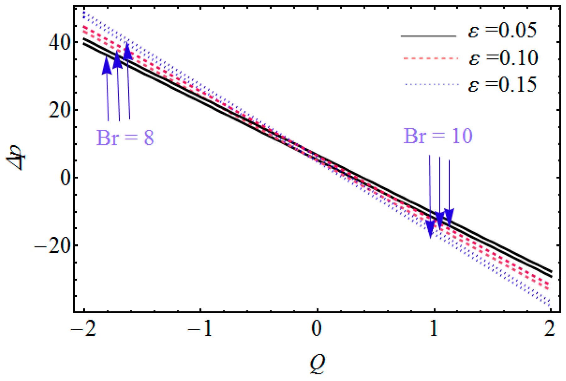
5. Results and Discussion

The authors obtained the quantitative analysis of nanoparticles in Jeffery fluid flowing past eccentric annuli having peristaltic waves at the outer surface. Heat and mass transfer phenomenon was also taken under consideration by the law of conservation of mass and energy. Lubrication theory was utilized to make the assumptions about laminar flow through arteries. Moreover, the effects of entropy generation and Bejan number were observed, which affect the flow due to irreversibility mechanism of temperature distribution, viscous dissipation, and nanoparticles’ concentration. In this section, we describe the effects of emerging physical parameters of obtaining quantities through figures which are drawn on Mathematica and ordered in a subsequent manner. Numerical data were achieved for the expression of pressure rise by using built-in commands in mathematical software. Table 1 is placed to find the variation of pressure rise data $\mathsf{\Delta }p,$ for a flow rate domain $Q$ from the interval $\left[–1,1\right],$ by varying the parameters $\delta$ and $Gr$ under the constant values of other factors. This table suggests that peristaltic pumping occurs at $Q=0$. Figure 2 and Figure 3 show the residual error curves, which clearly reflects the highly convergent solution of temperature distribution and nanoparticles’ concentration, respectively, by keeping the rest of the quantities numerically fixed. Moreover, the values used in the graph emphasized that we can assign these numerical values of the parameters involved. Figure 4 confirms the validation of current analysis by comparing the present analysis with the study Nadeem et al. [32], which was published for viscous fluid. From this figure it is quite obvious that the current study’s results were similar to the results obtained in [32] when we neglected the non-Newtonian effects by assigning a zero value to the Jeffrey fluid parameter ${\lambda }_1$. It was also found from this graph that for Jeffrey fluid the radial velocity reduces. This is due to the increase in shearing stress as ${\lambda }_1$ grows, which was introduced into the boundary layer, which can cause loss of speed.

Figure 5, Figure 6 and Figure 7 were plotted for pressure rise profile $\Delta p$ against the flow rate domain $Q$. Figure 5 evaluates the effects of two parameters, the inner radius of the annuli $\delta$, and the local temperature Grashof number $Gr$ on peristaltic pressure rise curves. From this figure we can imagine that the lines of $\Delta p$ are declining from left to right and intersecting each other at $Q=–0.2$. It can also be concluded here that pumping rate is increasing with both the parameters on the negative side of the domain, but reducing its inclination on the region of positive interval $\left[0,2\right]$. This is due to the fact that increasing the radius of the inner cylinder exerts greater pressure on the flow on the left side, as compared to the other one, due to the eccentricity of the two annuli. Moreover, an increase in the local temperature Grashof number is produced due to the increase in outer cylinder radius, thus producing more pumping on the left side, whilst keeping the other parameters uniform. Figure 6 is sketched for $\Delta p$ to estimate the influence of eccentricity parameter $\epsilon$ and the local nanoparticles Grashof number $Br$. One can observe clearly that a similar behavior is shown with $\epsilon$ and $Br$ in comparison to $\delta$ and $Gr$. The velocity profile can be considered in Figure 7 and Figure 8. Figure 7 discloses the variation of axial velocity $w$ against the radial coordinate $r$, which is plotted for increasing numerical values of eccentricity factor $\epsilon$ and inner cylinder velocity $V$. It is shown from this graph that when we speed up the inner cylinder, the maximum velocity of fluid gets reduced near the outer annulus surface, while an increase is noticed near the walls of the inner cylinder; also, under the impact of eccentricity of two cylinders, fluid enhances its speed, but near the lower walls it becomes stable, which is very much in line with the experimental and physical results. From Figure 8, we can predict that by enlarging the nanoparticle Grashof number $Gr$ and temperature Grashof number $Br$, the fluid travels rapidly in the space away from the lower surface, which is not closer to the lower boundary. Figure 9 and Figure 10 were included to find the theoretical characteristics of temperature distribution under the alteration of Brownian motion parameter $Nb$ and thermophoresis parameter $Nt$, correspondingly. It is obvious that, by raising the amount of both parameters, temperature of the liquid varied directly and the maximum temperature gradient was seen in the middle part of the space. This behavior clearly notifies that, in the presence of nanoparticles, the thermal conductivity of the fluid enhances significantly, which is also evident from the pioneer study on nanofluids [1]. This also suggests that the thermal conduction is caused by Brownian diffusion and thermophoresis diffusion in the rise of flow, which leads to an increase in flow temperature distribution.

The profile of nanoparticles $\sigma$ ismentioned in the diagrams labeled as Figure 11 and Figure 12. In Figure 11, we can see the effects of Brownian motion parameter $Nb$ on nanoparticles’ concentration. It is clearly seen from this graph that the amount of nanoparticles is lowered with the variation of $Nb$. Figure 12 reflects the curves of nanoparticles’ profile for the parameter $Nt$ and it can be suggested that nanoparticles’ concentration gets enlarged.

Figure 13, Figure 14, Figure 15, Figure 16, Figure 17 and Figure 18 exhibit the influence of emerging parameters on entropy function $Ns$. Figure 13 contains the graph of $Ns$ against the Brinkman number $Gc$. This figure implies that entropy generation increases near the lower surface of the space with the increasing effects of $Gc$, but in the wider part it gets lowered with the varying factor. It was noticed that the entropy of the system increases with the incursion in $Nb$ in most of the region, but near the walls it is almost stable (see Figure 14). Figure 15 concludes that the entropy shows similar characteristics with $Nt,$ as seen for $Nb,$ but an opposite result can be seen near the lower wall. This is because rising of $N_t$ involves larger viscous dissipation effects, due to energy production generating more entropy. From Figure 16 it can be visualized that entropy is proportional to the concentration difference parameter $\mathsf{\Omega }$ in the interval $r>0.5,$ but for $0<r<0.5$ an inverse relation is shown, but the ratio of temperature to concentration parameters $\mathsf{\Gamma }$ and the temperature difference parameter $\mathsf{\Lambda }$ showed increasing effects on the entropy generation, which can be confirmed from Figure 17 and Figure 18, accordingly.

Figure 19, Figure 20, Figure 21 and Figure 22 are established to show the effects of physical factors on Bejan number $Be$, which is the ratio of two entropy generations. Figure 19 elucidates that the increase in $Gc$ imposes an increase in Bejan number, which reflects the aspect that entropy due to heat transfer is less than that of total entropy in the lower region, but totally inverse readings are noted in the rest of the space. With the growing effects of $\mathsf{\Omega }$, Bejan number $Be$ enhances through the flow domain, which can be found in Figure 20. From Figure 21 and Figure 22 it is evident that $Be$ decreases with increments in $\mathsf{\Gamma }$ and $\mathsf{\Lambda },$ which indicates that the total entropy leads the same because of heat irreversibility.

6. Conclusions

In the current article, entropy generation analysis and Bejan number characteristics were investigated for peristaltic propulsion of Jeffrey fluid by introducing nanoparticles passing through two eccentric asymmetric annuli. Analytical solutions for velocity, temperature, and nanoparticles’ concentration were summarized. The pressure rise expression was evaluated numerically. Equations representing the laws of conservation were manipulated through the lubrication approach. The dimensionless phenomenon was also taken into account by incorporating some suitable transformations. Entropy generation number and Bejan number were achieved by substituting the obtained values of temperature distribution, velocity profile, and nanoparticles’ concentration. Effects of appertaining parameters were achieved by sketching diagrams. From the graphical features of the analysis, we gathered the following key observations:

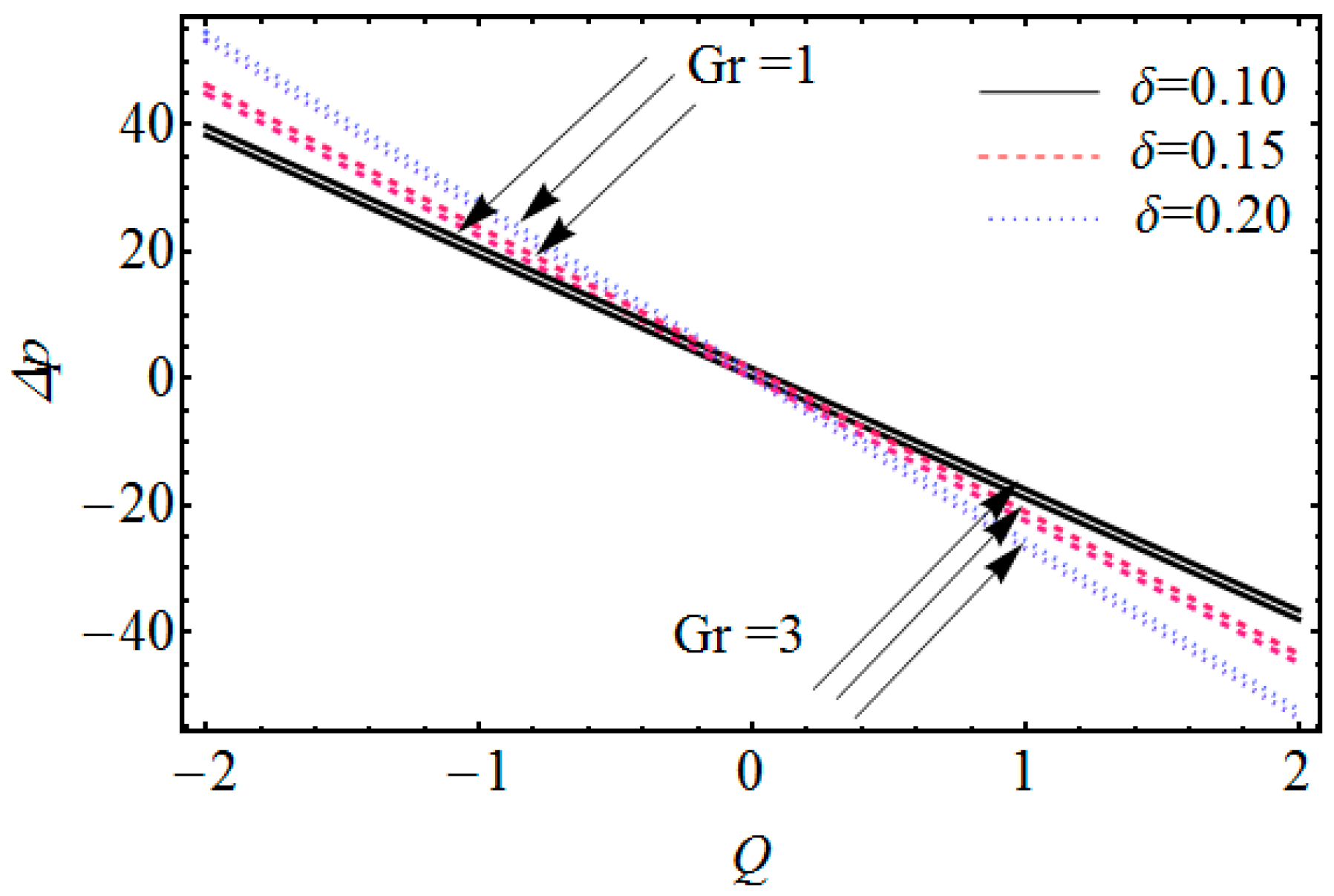
• The pumping rate increases under the growing contribution of nanoparticles’ Grashof number and temperature Grashof number.
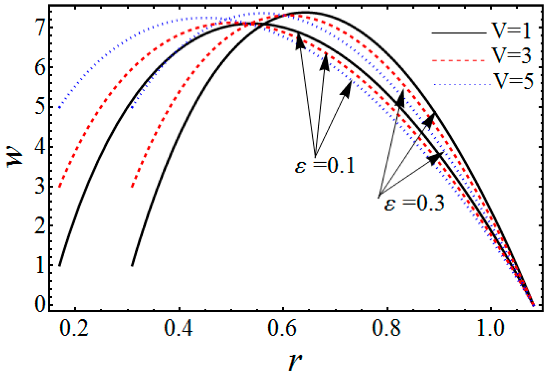
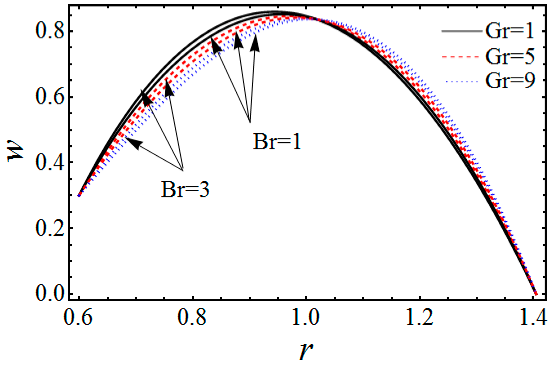
• The fluid travels rapidly when the inner cylinders move faster, but in the upper space fluid gets slow; on the other hand, there is an opposite response evaluated for local nanoparticles’ Grashof number as well as local temperature Grashof number.
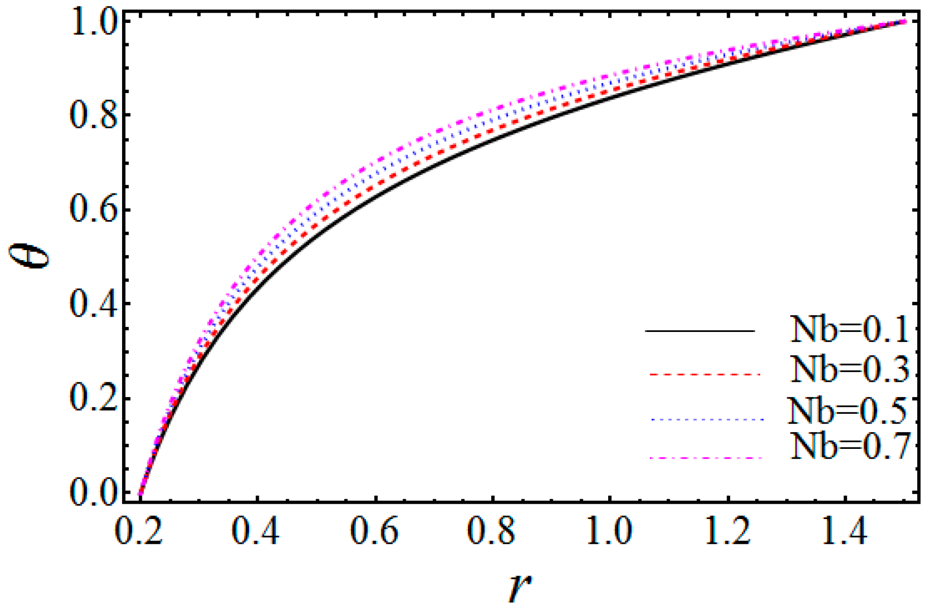
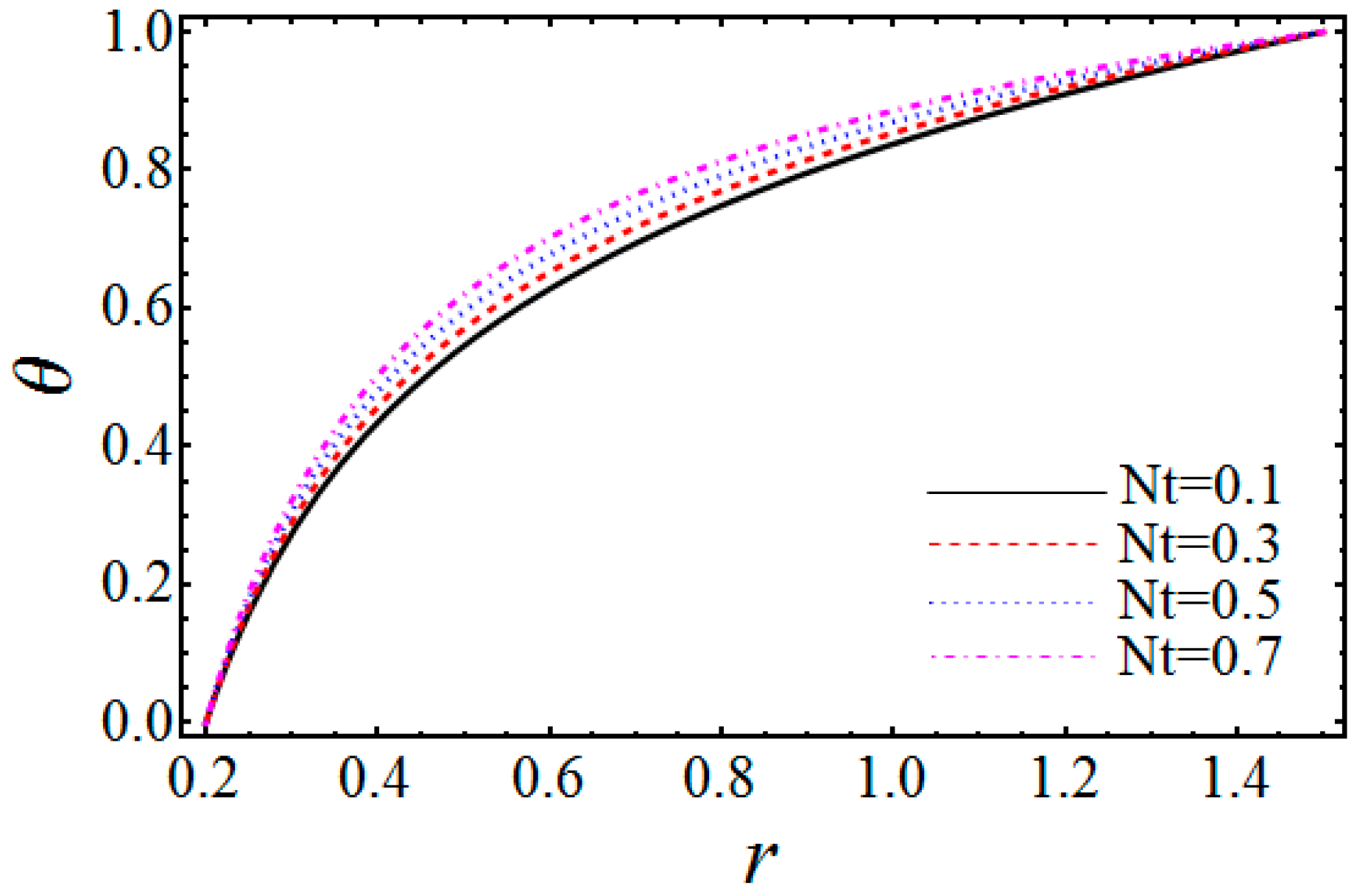
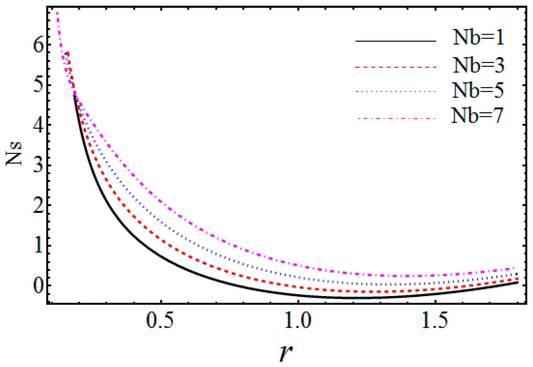
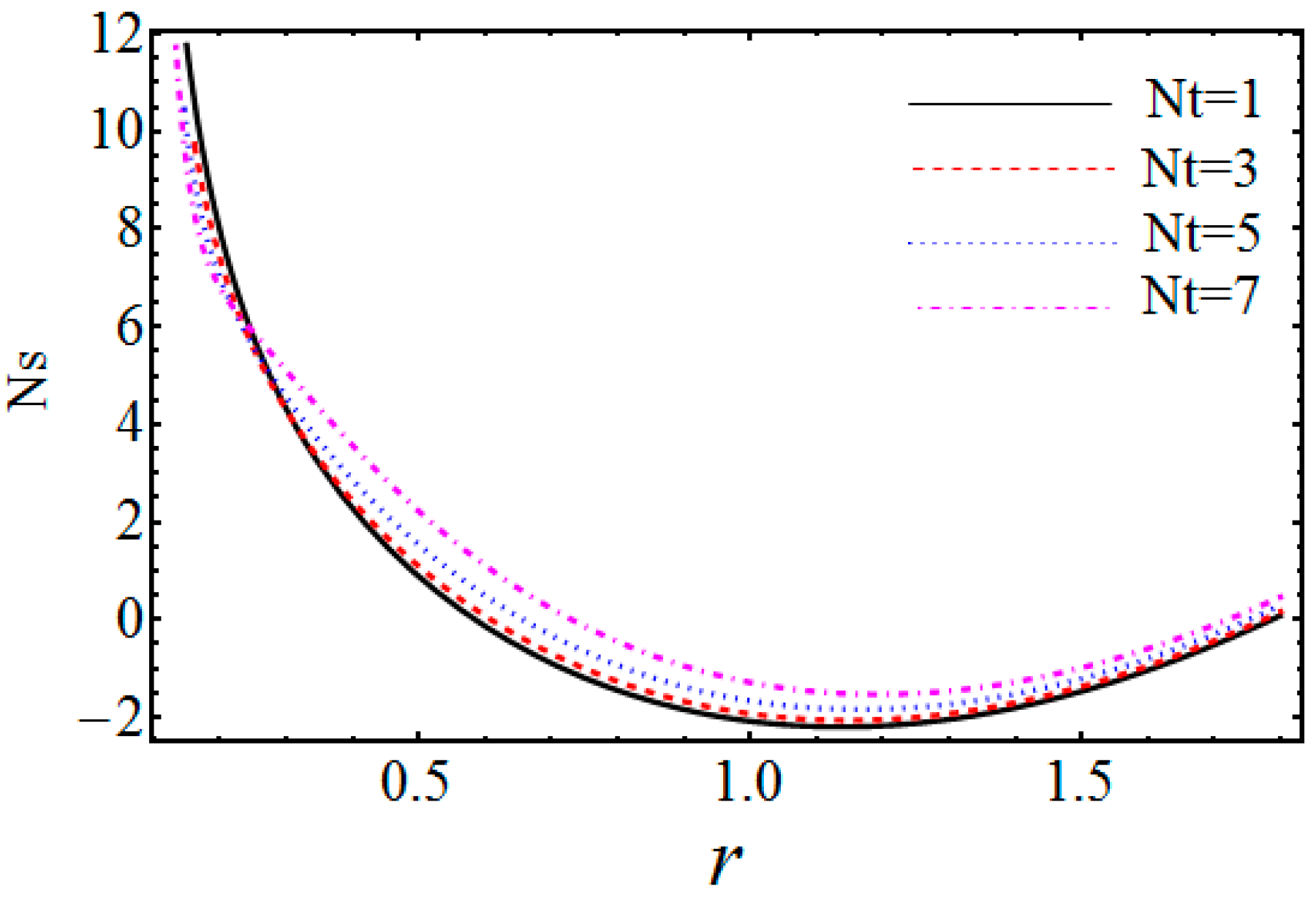
• It is shown that the flow gets more heated when we increase the magnitudes of the thermophoresis parameter and the Brownian motion parameter, which also indicates the increase in thermal conductivity of the material.
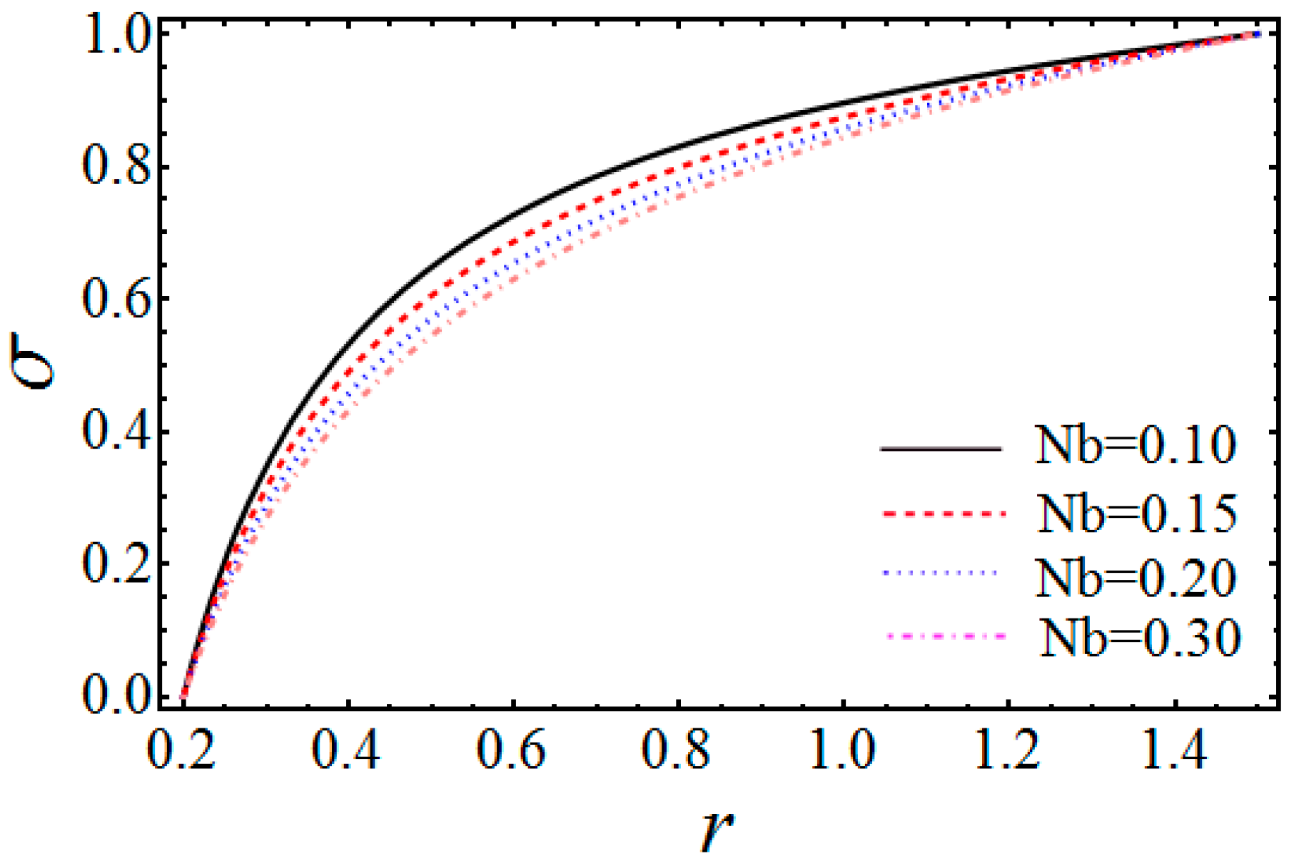
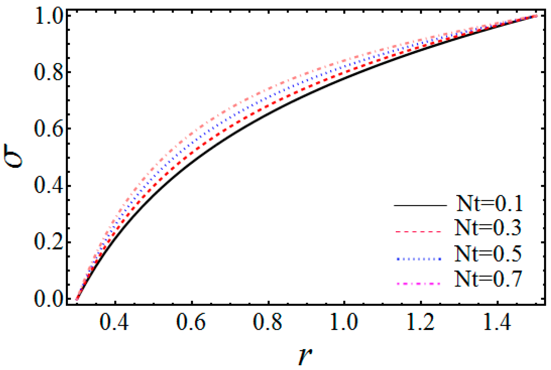
• It is estimated that nanoparticles enhance with the thermophoresis parameter, but reduce under the increasing effects of the Brownian motion factor.
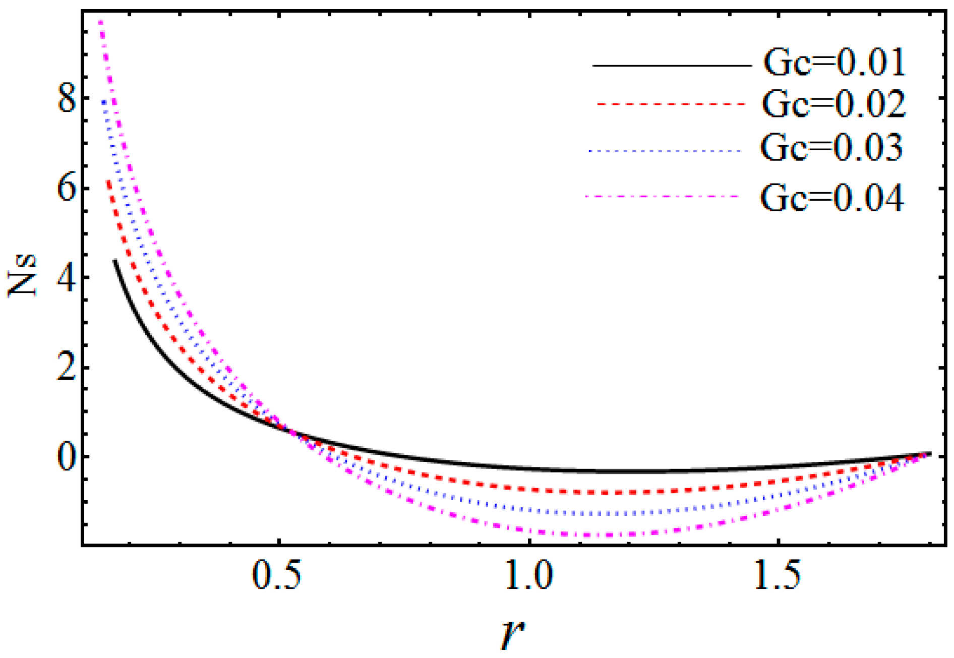
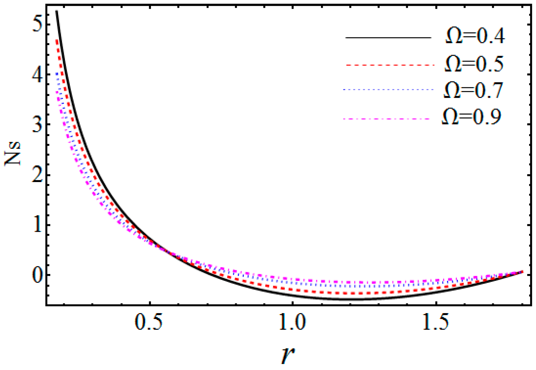
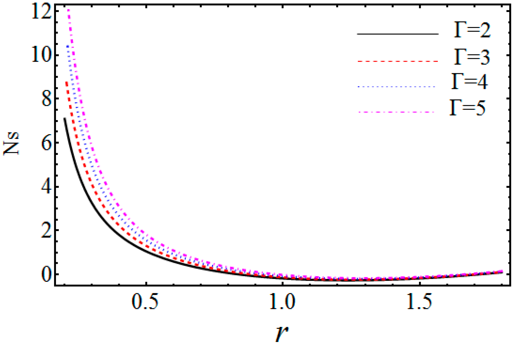
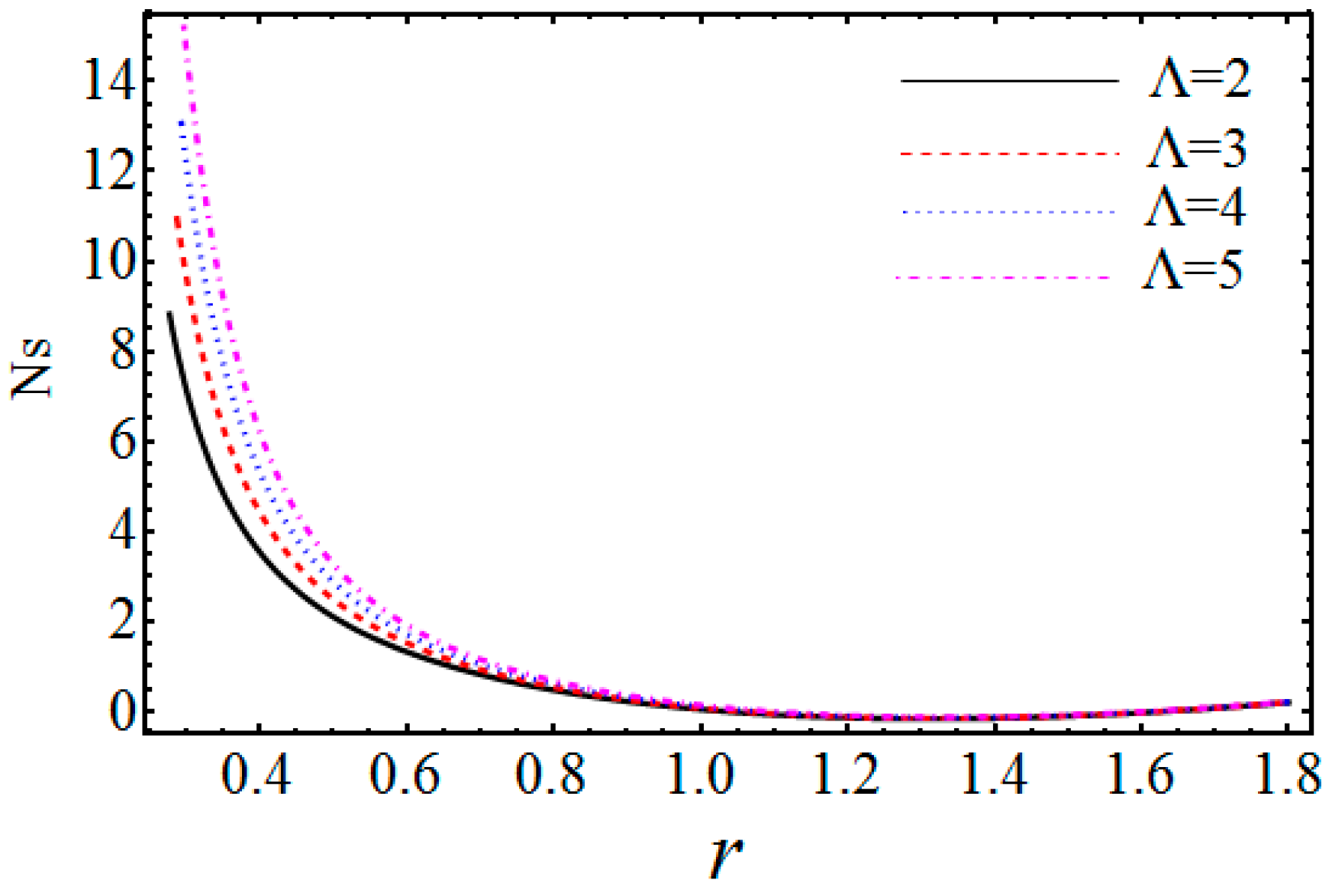
• It is summarized that entropy generation is raised near the inner cylinder when in relation to large values of Brinkman number; however, near the outer cylinder, observations are quite inverse; but against the thermophoresis parameter and Brownian motion parameter, entropy increased.
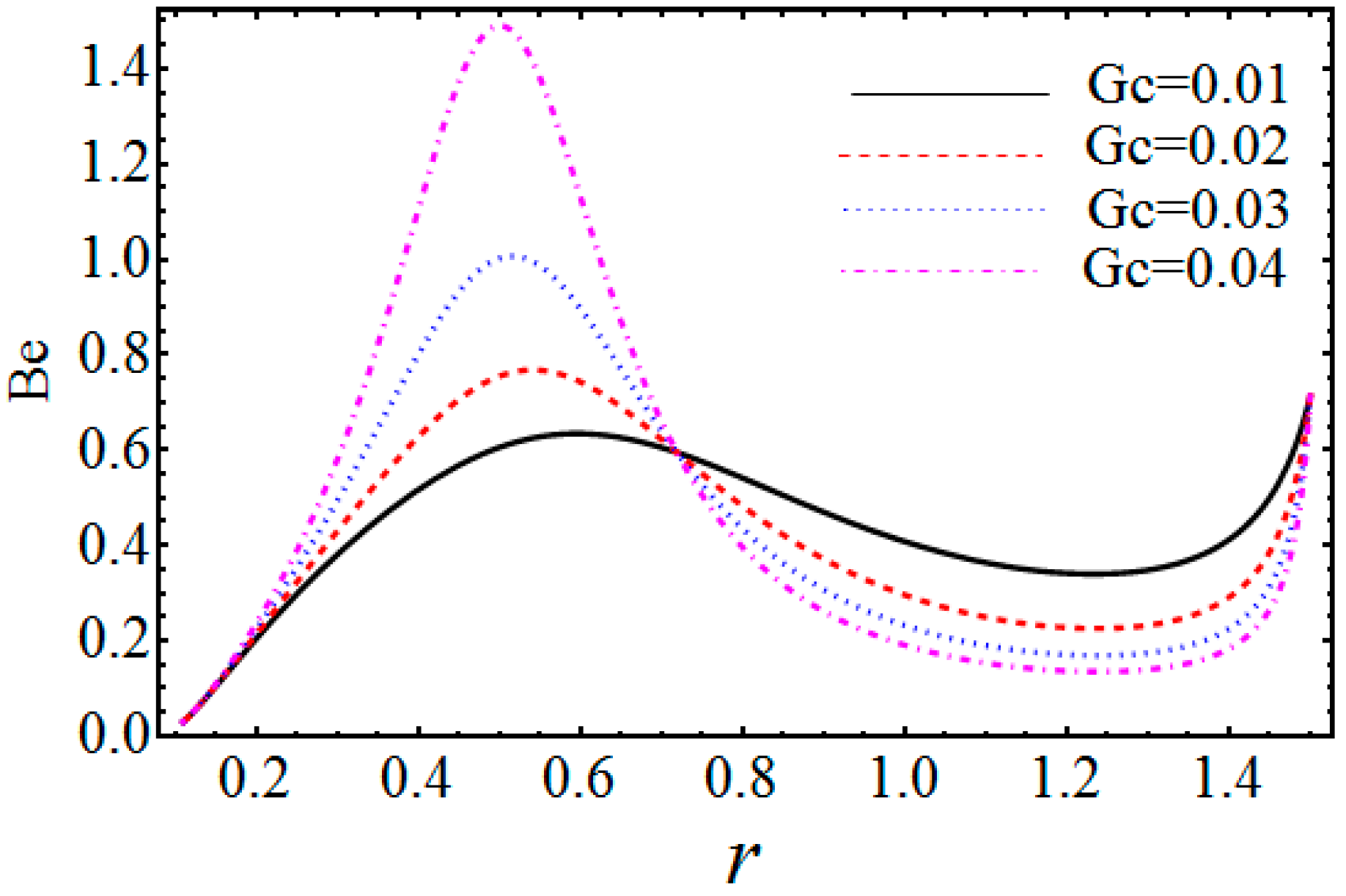
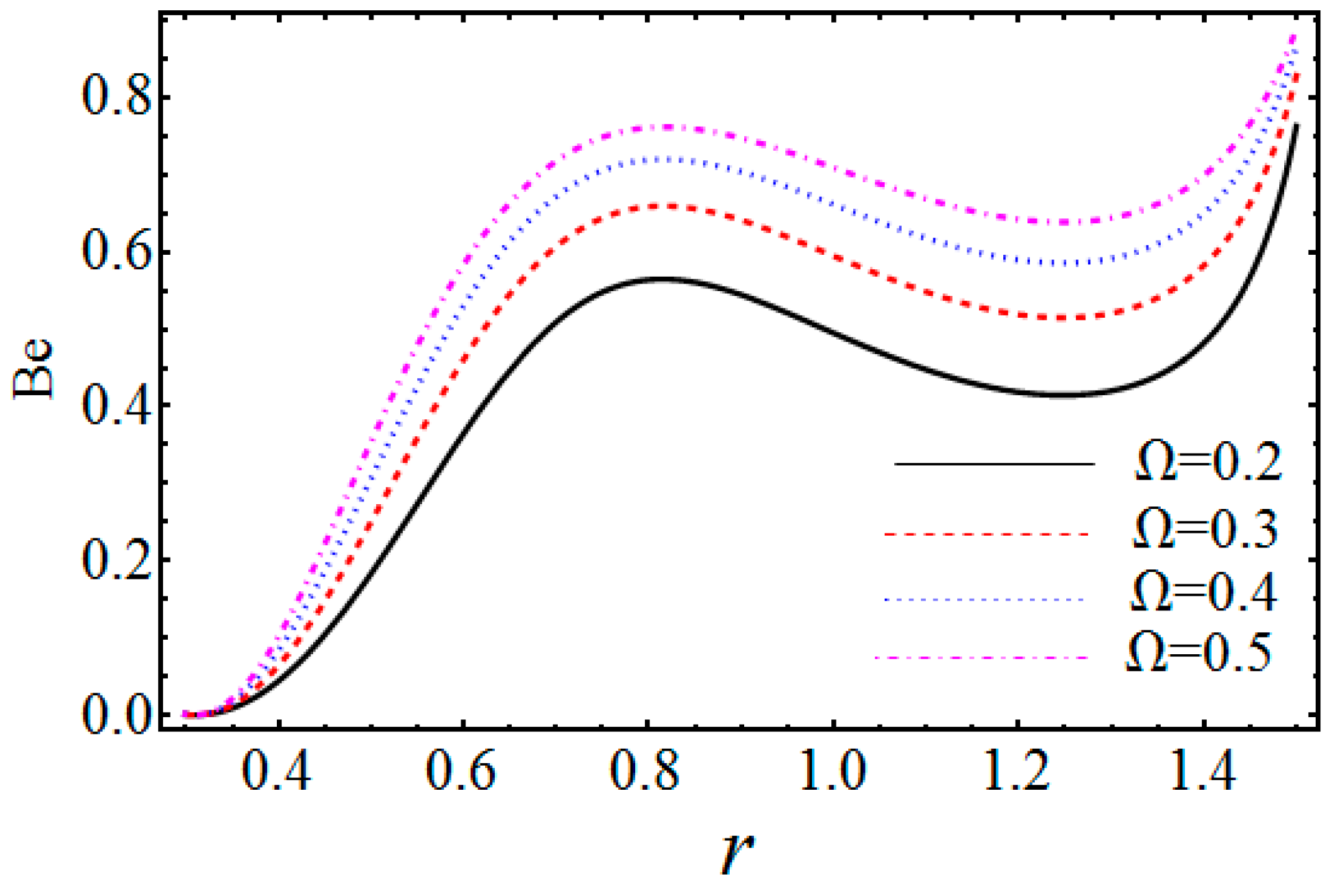
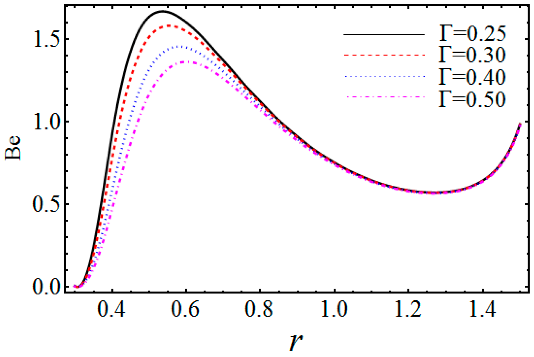
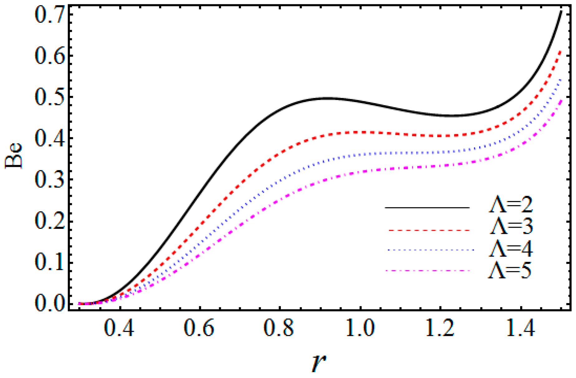
• From the figures of Bejan number, we showed that the temperature difference parameter and the ratio of temperature to concentration parameters degenerate the Bejan number, whereas the concentration difference parameter enhances the Bejan number; and the Brinkman number produces random results over the Bejan number profile.

References

1. Choi, S.U.S. Enhancing Thermal Conductivity of Fluids with Nanoparticles. In Proceedings of the ASME International Mechanical Engineering Congress and Exposition, Washington, DC, USA, 12–17 November 1995; Volume 66, pp. 99–105. [Google Scholar]
2. Alrashed, A.A.; Gharibdousti, M.S.; Goodarzi, M.; De Oliveira, L.R.; Safaei, M.R.; Filho, E.B. Effects on thermophysical properties of carbon based nanofluids: Experimental data, modelling using regression, ANFIS and ANN. Int. J. Heat Mass Transf. 2018, 125, 920–932. [Google Scholar] [CrossRef]
3. Long, G.; Liu, S.; Xu, G.; Wong, S.-W.; Chen, H.; Xiao, B. A Perforation-Erosion Model for Hydraulic-Fracturing Applications. SPE Prod. Oper. 2018, 33, 770–783. [Google Scholar] [CrossRef]
4. Xiao, B.; Wang, W.; Zhang, X.; Long, G.; Fan, J.; Chen, H.; Deng, L. A novel fractal solution for permeability and Kozeny-Carman constant of fibrous porous media made up of solid particles and porous fibers. Powder Technol. 2019, 349, 92–98. [Google Scholar] [CrossRef]
5. Xiao, B.; Zhang, X.; Jiang, G.; Long, G.; Wang, W.; Zhang, Y.; Liu, G.; Chen, H. Kozeny–carman constant for gas flow through fibrous porous media by fractal-monte carlo simulations. Fractals 2019, 27, 27. [Google Scholar] [CrossRef]
6. Cao, Y.; Irwin, P.; Younsi, K. The future of nanodielectrics in the electrical power industry. IEEE Trans. Dielectr. Electr. Insul. 2004, 11, 797–807. [Google Scholar]
7. Imai, T.; Sawa, F.; Ozaki, T.; Shimizu, T.; Kuge, S.-I.; Kozako, M.; Tanaka, T. Approach by Nano- and Micro-filler Mixture toward Epoxy-based Nanocomposites as Industrial Insulating Materials. IEEJ Trans. Fundam. Mater. 2006, 126, 1136–1143. [Google Scholar] [CrossRef] [Green Version]
8. Amiri, S.; Shokrollahi, H. The role of cobalt ferrite magnetic nanoparticles in medical science. Mater. Sci. Eng. C 2013, 33, 1–8. [Google Scholar] [CrossRef]
9. Prabhu, S.; Poulose, E.K. Silver nanoparticles: Mechanism of antimicrobial action, synthesis, medical applications, and toxicity effects. Int. Nano Lett. 2012, 2, 32. [Google Scholar] [CrossRef] [Green Version]
10. Hanahan, U.; Weinberg, R.A. The Hallmarks of Cancer. Cell 2000, 100, 57–70. [Google Scholar] [CrossRef] [Green Version]
11. Prakash, J.; Siva, E.; Tripathi, D.; Kothandapani, M. Nanofluids flow driven by peristaltic pumping in occurrence of magnetohydrodynamics and thermal radiation. Mater. Sci. Semicond. Process. 2019, 100, 290–300. [Google Scholar] [CrossRef]
12. Abbas, M.A.; Bai, Y.-Q.; Rashidi, M.M.; Bhatti, M.M. Analysis of Entropy Generation in the Flow of Peristaltic Nanofluids in Channels With Compliant Walls. Entropy 2016, 18, 90. [Google Scholar] [CrossRef]
13. Abdelsalam, S.I.; Bhatti, M.M. The study of non-Newtonian nanofluid with hall and ion slip effects on peristaltically induced motion in a non-uniform channel. RSC Adv. 2018, 8, 7904–7915. [Google Scholar] [CrossRef] [Green Version]
14. Shah, Z.; Khan, A.; Khan, W.; Alam, M.K.; Islam, S.; Kuma, P.; Thounthong, P. Micropolar gold blood nanofluid flow and radiative heat transfer between permeable channels. Comput. Methods Programs Biomed. 2020, 186, 105197. [Google Scholar] [CrossRef] [PubMed]
15. Bhatti, M.M.; Zeeshan, A.; Ellahi, R.; Bég, O.A.; Kadir, A. Effects of coagulation on the two-phase peristaltic pumping of magnetized prandtl biofluid through an endoscopic annular geometry containing a porous medium. Chin. J. Phys. 2019, 58, 222–234. [Google Scholar] [CrossRef]
16. Kume, K. Endoscopic mucosal resection and endoscopic submucosal dissection for early gastric cancer: Current and original devices. World J. Gastrointest. Endosc. 2009, 1, 21–31. [Google Scholar] [CrossRef] [PubMed]
17. Kahshan, M.; Lu, D.; Siddiqui, A.M. A Jeffrey Fluid Model for a Porous-walled Channel: Application to Flat Plate Dialyzer. Sci. Rep. 2019, 9, 15879. [Google Scholar] [CrossRef] [PubMed] [Green Version]
18. Pandey, S.K.; Tripathi, D. Unsteady model of transportation of jeffrey-fluid by peristalsis. Int. J. Biomath. 2010, 3, 473–491. [Google Scholar] [CrossRef]
19. Ellahi, R.; Bhatti, M.M.; Pop, I. Effects of hall and ion slip on MHD peristaltic flow of Jeffrey fluid in a non-uniform rectangular duct. Int. J. Numer. Methods Heat Fluid Flow 2016, 26, 1802–1820. [Google Scholar] [CrossRef]
20. Ramesh, K.; Tripathi, D.; Beg, O.A.; Kadir, A. Slip and hall current effects on Jeffrey fluid suspension flow in a peristaltic hydromagnetic blood micro pump. Iran. J. Sci. Technol. Trans. Mech. Eng. 2019, 43, 675–692. [Google Scholar] [CrossRef]
21. Ranjit, N.K.; Shit, G. Entropy generation on electro-osmotic flow pumping by a uniform peristaltic wave under magnetic environment. Energy 2017, 128, 649–660. [Google Scholar] [CrossRef]
22. Ellahi, R.; Hussain, F.; Ishtiaq, F.; Hussain, A. Peristaltic transport of Jeffrey fluid in a rectangular duct through a porous medium under the effect of partial slip: An application to upgrade industrial sieves/filters. Pramana 2019, 93, 34. [Google Scholar] [CrossRef]
23. Zeeshan, A.; Ijaz, N.; Abbas, T.; Ellahi, R. The Sustainable Characteristic of Bio-Bi-Phase Flow of Peristaltic Transport of MHD Jeffrey Fluid in the Human Body. Sustainability 2018, 10, 2671. [Google Scholar] [CrossRef] [Green Version]
24. Ellahi, R.; Zeeshan, A.; Hussain, F.; Asadollahi, A. Peristaltic Blood Flow of Couple Stress Fluid Suspended with Nanoparticles under the Influence of Chemical Reaction and Activation Energy. Symmetry 2019, 11, 276. [Google Scholar] [CrossRef] [Green Version]
25. Mekheimer, K.S.; Elmaboud, Y.A.; Abdellateef, A.I. Particulate suspension flow induced by sinusoidal peristaltic waves through eccentric cylinders: Thread annular. Int. J. Biomath. 2013, 6, 1350026. [Google Scholar] [CrossRef]
26. Pakdemirli, M.; Yilbas, B.S. Entropy generation in a pipe due to non-Newtonian fluid flow: Constant viscosity case. Sadhana 2006, 31, 21–29. [Google Scholar] [CrossRef] [Green Version]
27. Souidi, K.F.; Ayachi, N. BenyahiaEntropy generation rate for a peristaltic pump. J. Non Equilib. Thermodyn. 2009, 34, 171–194. [Google Scholar] [CrossRef]
28. Abu-Nada, E. Entropy generation due to heat and fluid flow in backward facing step flow with various expansion ratios. Int. J. Exergy 2006, 3, 419. [Google Scholar] [CrossRef] [Green Version]
29. Bibi, A.; Xu, H. Entropy Generation Analysis of Peristaltic Flow and Heat Transfer of a Jeffery Nanofluid in a Horizontal Channel under Magnetic Environment. Math. Probl. Eng. 2019, 2019, 1–13. [Google Scholar] [CrossRef] [Green Version]
30. Rashidi, M.M.; Bhatti, M.M.; Abbas, M.A.; Ali, M. Entropy Generation on MHD Blood Flow of Nanofluid Due to Peristaltic Waves. Entropy 2016, 18, 117. [Google Scholar] [CrossRef] [Green Version]
31. Ellahi, R.; Raza, M.; Akbar, N.S. Study of peristaltic flow of nanofluid with entropy generation in a porous medium. J. Porous Media 2017, 20, 461–478. [Google Scholar] [CrossRef]
32. Nadeem, S.; Riaz, A.; Ellahi, R.; Akbar, N.S. Effects of heat and mass transfer on peristaltic flow of a nanofluid between eccentric cylinders. Appl. Nanosci. 2013, 4, 393–404. [Google Scholar] [CrossRef] [Green Version]
33. Jamalabadi, M.Y.A.; DaqiqShirazi, M.; Nasiri, H.; Safaei, M.R.; Nguyen, T.-N. Modeling and analysis of biomagnetic blood Carreau fluid flow through a stenosis artery with magnetic heat transfer: A transient study. PLoS ONE 2018, 13, e0192138. [Google Scholar]
34. Maleki, H.; Alsarraf, J.; Moghanizadeh, A.; Hajabdollahi, H.; Safaei, M.R. Heat transfer and nanofluid flow over a porous plate with radiation and slip boundary conditions. J. Central South Univ. 2019, 26, 1099–1115. [Google Scholar] [CrossRef]
35. He, J.-H. Homotopy perturbation method for solving boundary value problems. Phys. Lett. A 2006, 350, 87–88. [Google Scholar] [CrossRef]
36. Riaz, A.; Alolaiyan, H.; Razaq, A. Convective Heat Transfer and Magnetohydrodynamics across a Peristaltic Channel Coated with Nonlinear Nanofluid. Coatings 2019, 9, 816. [Google Scholar] [CrossRef] [Green Version]
37. Alolaiyan, H.; Riaz, A.; Razaq, A.; Saleem, N.; Zeeshan, A.; Bhatti, M.M. Effects of Double Diffusion Convection on Third Grade Nanofluid through a Curved Compliant Peristaltic Channel. Coatings 2020, 10, 154. [Google Scholar] [CrossRef] [Green Version]
Figure 1. Diagram of flow mechanism and annuli.
Coatings 10 00213 g001
Figure 2. Residual error curves of temperature distribution θ .
Coatings 10 00213 g002
Figure 3. Residual error curves of nanoparticles’ concentration σ
Coatings 10 00213 g003
Figure 4. Comparison of present study with [32].
Coatings 10 00213 g004
Figure 5. Variation of pressure rise Δ p with δ and G r for fixed θ = 0.8 ,     φ = 0.1 ,   ε = 0.1 ,   B r = 0.2 ,   N b = 0.5 ,   N t = 0.2 ,   λ 1 = 5 ,   V = 0.1 ,   t = 0.05 . .
Coatings 10 00213 g005
Figure 6. Variation of pressure rise Δ p   with ε and B r for fixed θ = 0.8 ,     φ = 0.1 ,   δ = 0.1 ,   G r = 0.2 ,   N b = 0.5 ,   N t = 0.2 ,   λ 1 = 5 ,   V = 0.1 ,   t = 0.05 . .
Coatings 10 00213 g006
Figure 7. Variation of velocity profile w with ε and V for fixed θ = 0.8 ,     φ = 0.1 ,   δ = 0.1 ,   B r = 0.3 ,   G r = 1 ,     λ 1 = 1 ,   z = 0 ,   t = 0.1 ,   Q = 1 .   .
Coatings 10 00213 g007
Figure 8. Variation of velocity profile w with B r and G r for fixed θ = 0.1 ,     φ = 0.5 ,   δ = 0.5 ,   ε = 0.1 ,   V = 0.3 ,     λ 1 = 0.7 ,   z = 0 ,   t = 0.1 ,   Q = 1 .   .
Coatings 10 00213 g008
Figure 9. Variation of temperature profile θ ¯ with N b for fixed θ = 0.1 ,     φ = 0.5 ,   δ = 0.1 ,   ε = 0.1 ,     V = 0.3 ,     λ 1 = 0.7 ,   z = 0 ,   t = 0.3 ,   N t = 0.2 ,   B r = 0.5 . .
Coatings 10 00213 g009
Figure 10. Variation of temperature profile θ ¯ with N t for fixed θ = 0.1 ,     φ = 0.5 ,   δ = 0.1 ,   ε = 0.1 ,     V = 0.3 ,     λ 1 = 1 ,   z = 0 ,   t = 0.3 ,   N b = 0.2 ,   B r = 0.5 .
Coatings 10 00213 g010
Figure 11. Variation of nanoparticles phenomenon σ   with N b for fixed θ = 0.1 ,     φ = 0.5 ,   δ = 0.1 ,   ε = 0.1 ,   z = 0 ,   t = 0.3 ,   N t = 0.2 . .
Coatings 10 00213 g011
Figure 12. Variation of temperature profile σ   with N t for fixed θ = 0.1 ,     φ = 0.5 ,   δ = 0.2 ,   ε = 0.1 ,   z = 0 ,   t = 0.2 ,   N b = 0.2 . .
Coatings 10 00213 g012
Figure 13. Curves of N s with fixed G c where θ = 0.1 ,     φ = 0.5 ,   δ = 0.01 ,   ε = 0.01 ,   V = 0.3 ,     λ 1 = 1 ,   z = 0 ,   t = 0.1 ,   Γ = 0.4 ,   N b = 0.9 ,   N t = 0.5 ,   B r = 1 ,   G r = 3 ,   Λ = 0.4 ,   Ω = 0.3 ,   Q = 1 .   .
Coatings 10 00213 g013
Figure 14. Curves of N s with fixed N b where θ = 0.1 ,     φ = 0.8 ,   δ = 0.01 ,   ε = 0.01 ,   V = 0.3 ,     λ 1 = 1 ,   z = 0 ,   t = 0.1 ,   Γ = 0.4 ,   G c = 0.01 ,   N t = 0.9 ,   B r = 1 ,   G r = 3 ,   Λ = 1 ,   Ω = 0.3 ,   Q = 1 .   .
Coatings 10 00213 g014
Figure 15. Curves of N s with fixed N t where θ = 0.1 ,     φ = 0.8 ,   δ = 0.01 ,   ε = 0.01 ,   V = 0.3 ,     λ 1 = 1 ,   z = 0 ,   t = 0.1 ,   Γ = 0.4 ,   G c = 0.05 ,   N b = 0.9 ,   B r = 1 ,   G r = 3 ,   Λ = 1 ,   Ω = 0.3 ,   Q = 1 .   .
Coatings 10 00213 g015
Figure 16. Curves of N s with fixed Ω where θ = 0.1 ,     φ = 0.8 ,   δ = 0.01 ,   ε = 0.01 ,   V = 0.3 ,     λ 1 = 1 ,   z = 0 ,   t = 0.1 ,   Γ = 0.4 ,   G c = 0.01 ,   N t = 0.5 ,   B r = 1 ,   G r = 5 ,   Λ = 1 ,   N b = 0.9 ,   Q = 1 .   .
Coatings 10 00213 g016
Figure 17. Curves of N s   with fixed Γ where θ = 0.3 ,     φ = 0.8 ,   δ = 0.01 ,   ε = 0.01 ,   V = 0.3 ,     λ 1 = 1 ,     z = 0 ,   t = 0.1 ,   Ω = 0.3 ,   G c = 0.01 ,   N t = 0.5 ,   B r = 1 ,   G r = 3 ,   Λ = 0.4 ,   N b = 0.9 ,   Q = 1 . .
Coatings 10 00213 g017
Figure 18. Curves of N s with fixed Λ where θ = 0.3 ,     φ = 0.8 ,   δ = 0.01 ,   ε = 0.01 ,   V = 0.3 ,     λ 1 = 1 ,   z = 0 ,   t = 0.1 ,   Ω = 0.3 ,   G c = 0.01 ,   N t = 0.5 ,   B r = 1 ,   G r = 3 ,   Γ = 0.4 ,   N b = 0.9 ,   Q = 1 . .
Coatings 10 00213 g018
Figure 19. Curves of B e with fixed G c where θ = 0.1 ,     φ = 0.5 ,   δ = 0.1 ,   ε = 0.01 ,   V = 0.3 ,     λ 1 = 0.1 ,   z = 0 ,   t = 0.1 ,   Ω = 0.3 ,   Λ = 1 ,   N t = 0.5 ,   B r = 1 ,   G r = 5 ,   Γ = 0.4 ,   N b = 0.9 ,   Q = 1 . .
Coatings 10 00213 g019
Figure 20. Curves of B e with fixed Ω where θ = 0.1 ,     φ = 0.5 ,   δ = 0.1 ,   ε = 0.2 ,   V = 0.3 ,     λ 1 = 0.1 ,     z = 0 ,   t = 0.1 ,   G c = 0.01 ,   Λ = 1 ,   N t = 0.5 ,   B r = 1 ,   G r = 5 ,   Γ = 0.4 ,   N b = 0.9 ,   Q = 1 . .
Coatings 10 00213 g020
Figure 21. Curves of B e with fixed Γ where θ = 0.1 ,     φ = 0.5 ,   δ = 0.1 ,   ε = 0.2 ,   V = 0.3 ,     λ 1 = 0.1 ,     z = 0 ,   t = 0.1 ,   G c = 0.01 ,   Λ = 1 ,   N t = 0.5 ,   B r = 1 ,   G r = 5 ,   Ω = 0.3 ,   N b = 0.9 ,   Q = 1 . .
Coatings 10 00213 g021
Figure 22. Curves of B e with fixed Λ where θ = 0.1 ,     φ = 0.5 ,   δ = 0.1 ,   ε = 0.2 ,   V = 0.3 ,     λ 1 = 0.1 ,     z = 0 ,   t = 0.1 ,   G c = 0.01 ,   Γ = 0.4 ,   N t = 0.5 ,   B r = 1 ,   G r = 5 ,   Ω = 0.3 ,   N b = 0.9 ,   Q = 1 . .
Coatings 10 00213 g022