Label-Free Differentiation of Cancer and Non-Cancer Cells Based on Machine-Learning-Algorithm-Assisted Fast Raman Imaging


Abstract
:1. Introduction
2. Materials’ Preparation and Analytical Methods
2.1. Cell Culturing Process
2.2. Confocal Raman Spectroscopy Measurement
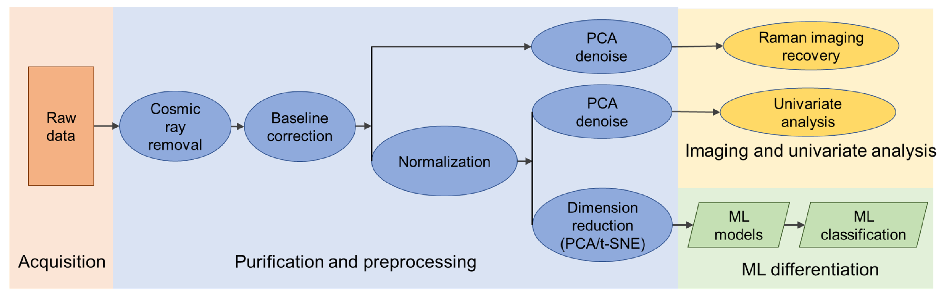
2.3. Data Processing Workflow
2.4. Machine Learning Models and Predictions
3. Results and discussion
3.1. Identification of Potential Raman Signature Bands

| Wavenumber (cm) | Bands’ Assignment |
|---|---|
| 719 | Phospholipid (choline) [42] |
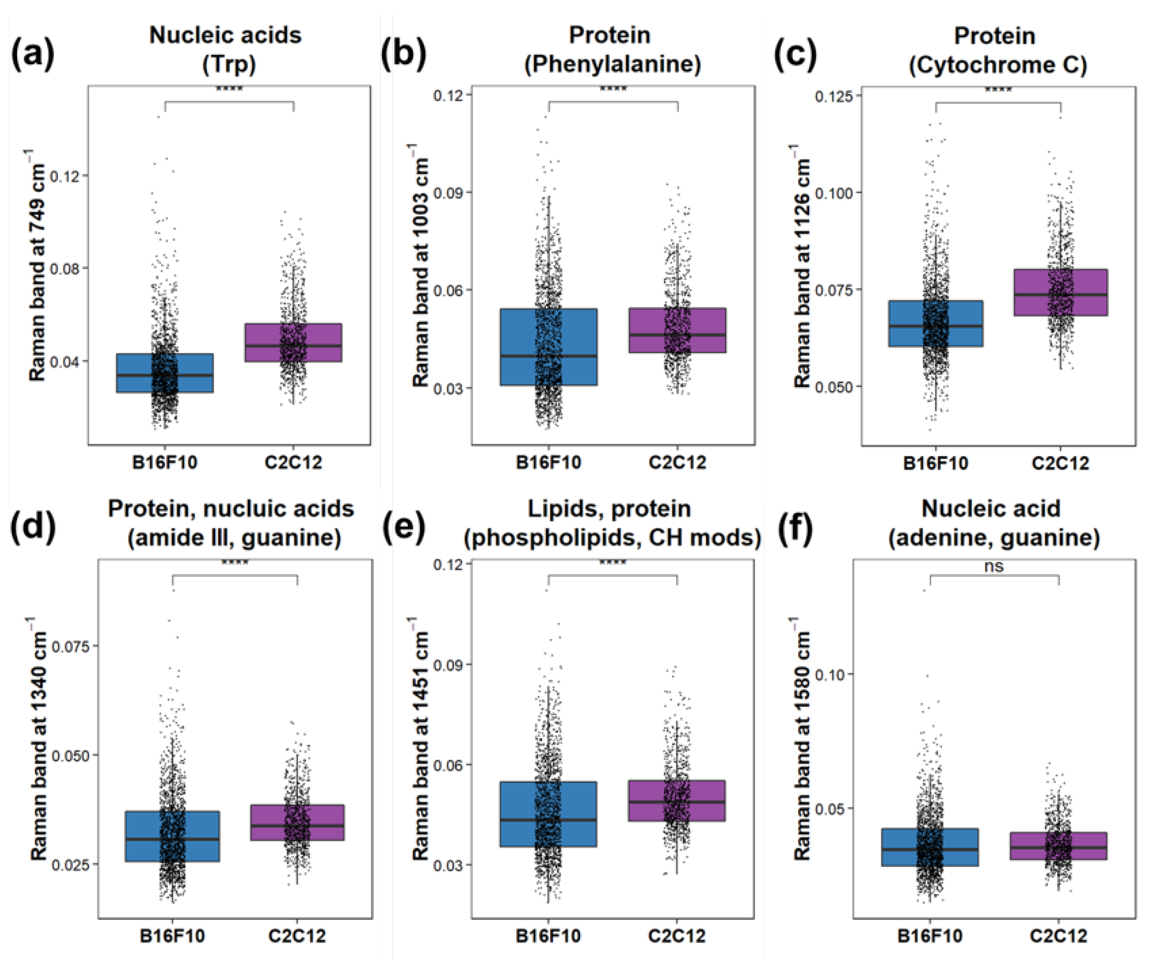
| 749 | Nucleic acids, Trp |
| 825 | Lactic acid |
| 858 | Glycans, N-acetyloglucosamine, O-S-O (GAG), glycogen |
| 895 | Glycans |
| 917 | C-C stretching of proline, glucose, lactic acid [43] |
| 925 | Glycans, glycogen, N-acetyloglucosamine |
| 1003 | Phenylalanine [44], symmetric ring breathing of protein [45] |
| 1064 | Lipids/collagen [46,47] C-C str |
| 1091 | Phospholipids [46], O-P-O symmetric stretching, |
| P=O symmetric vibration from nucleic acids/cell membrane | |
| phospholipids | |
| 1126 | Cytochrome C |
| 1304 | Lipids, phospholipids [46] C-H2 twist, collagen, protein amide III, DNA [43] |
| 1340 | Amide III; CH vibrations (CH2 and CH3 wagging) of proteins; |
| C-C stretching of aromatic ring (proteins); | |
| Melanin (C-C stretching of aromatic ring and C-H bending—broadband); | |
| Nucleic acids (guanine); actin [48] | |
| 1451 | Proteins [46] C-H wag, CH2, or CH3 def. phospholipids, CH2 scissoring [49] |
| 1580 | Adenine, guanine (DNA and RNA base) [50] |
| 1651 | (C=C) stretching, unsaturated fatty acids, triglycerides |
| 1656 | (C=C) stretching [51], Amide I α-helix (amino acids) |
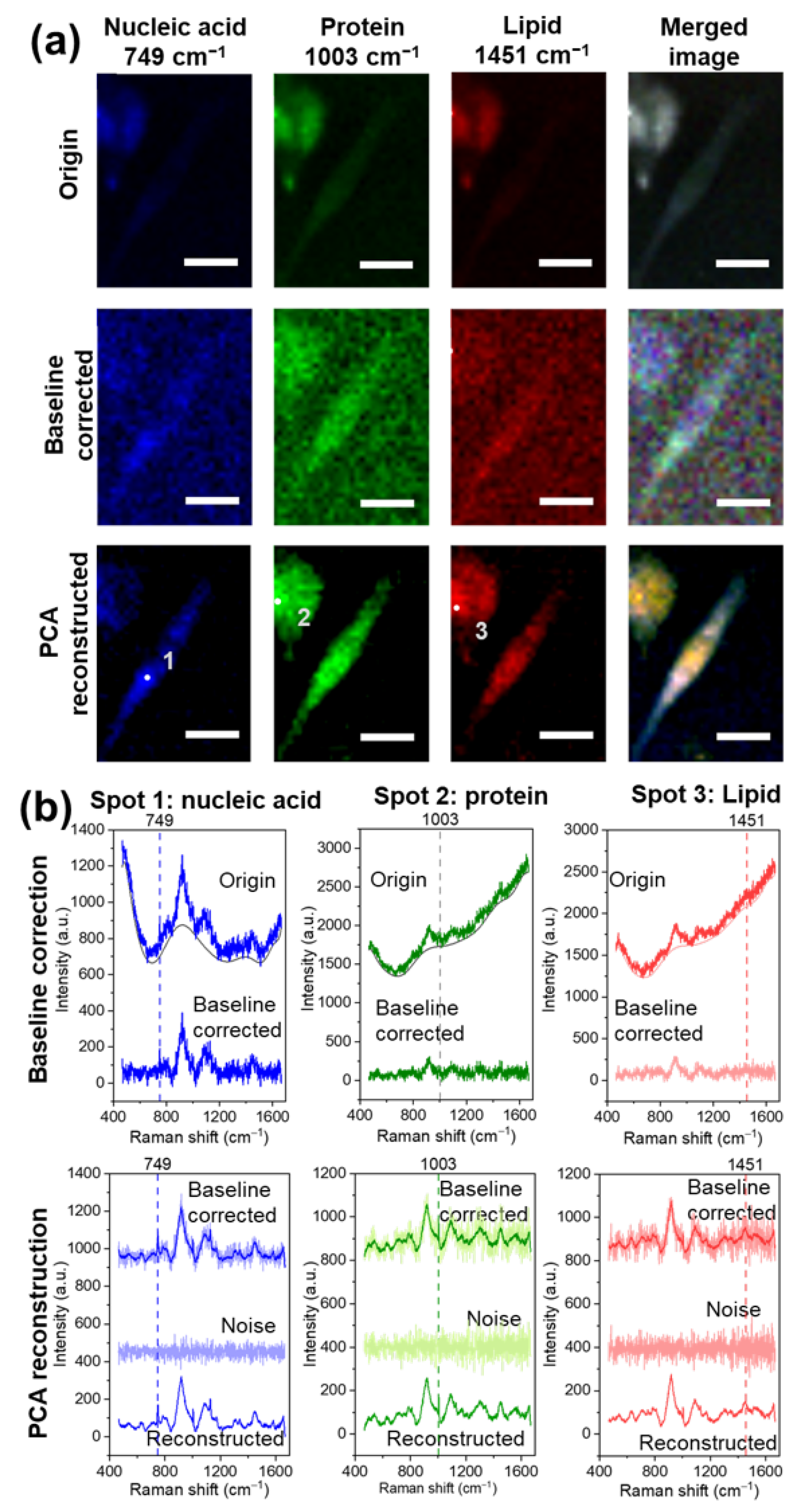
3.2. Purification and Reconstruction of the Raman Dataset
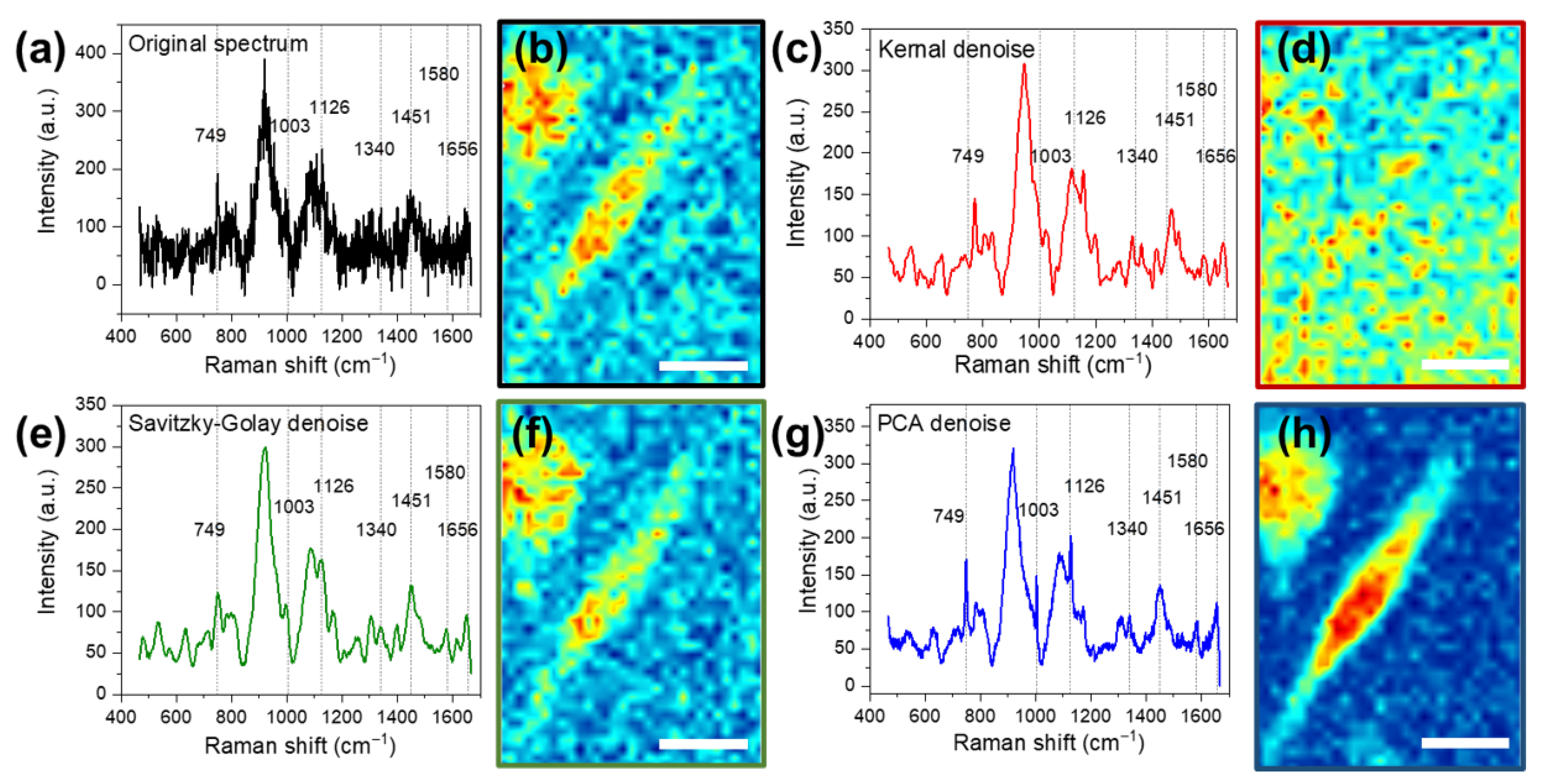
3.3. Comparison of PCA with Traditional Denoising Algorithms
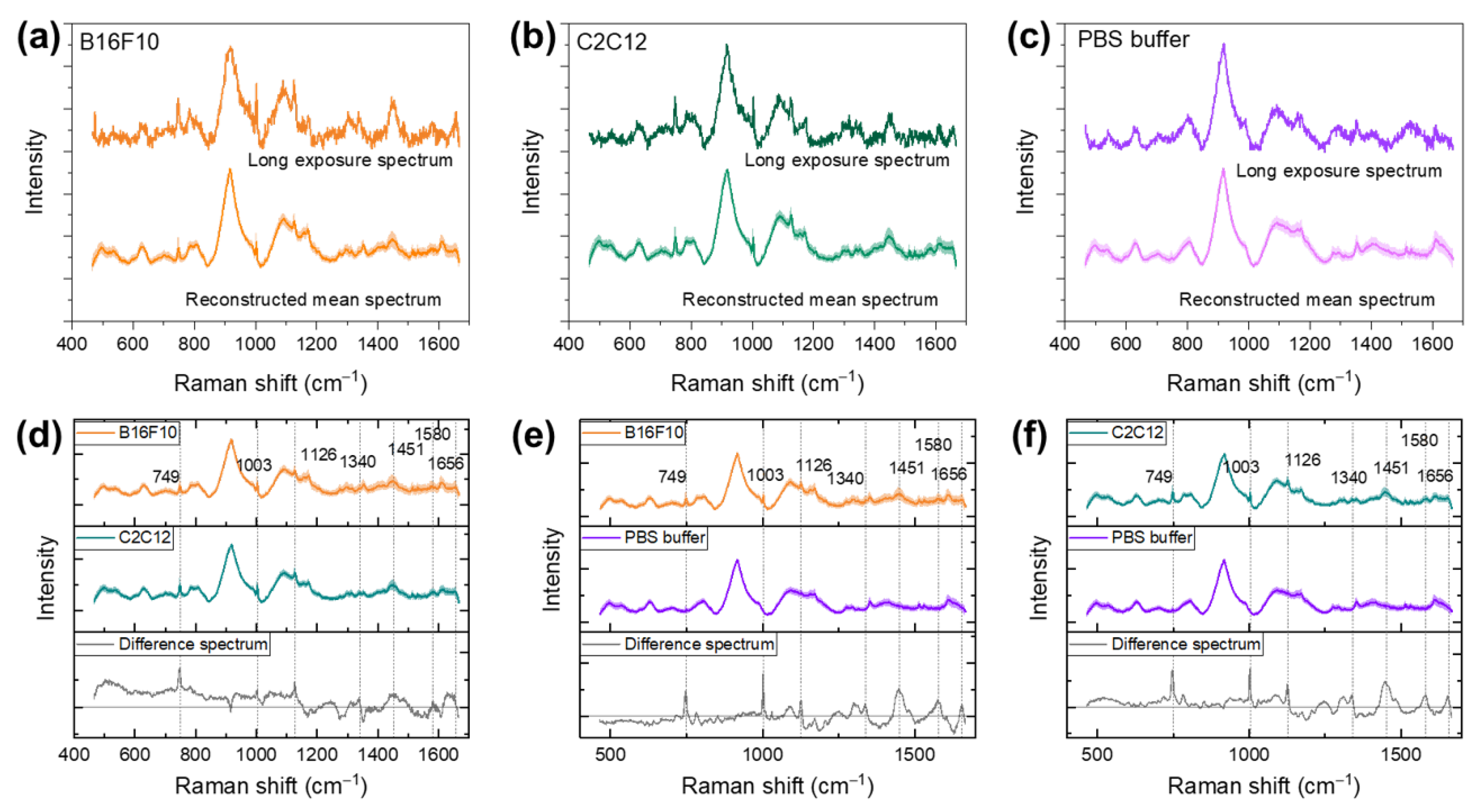
3.4. Univariate Analysis of Biomolecules’ Content
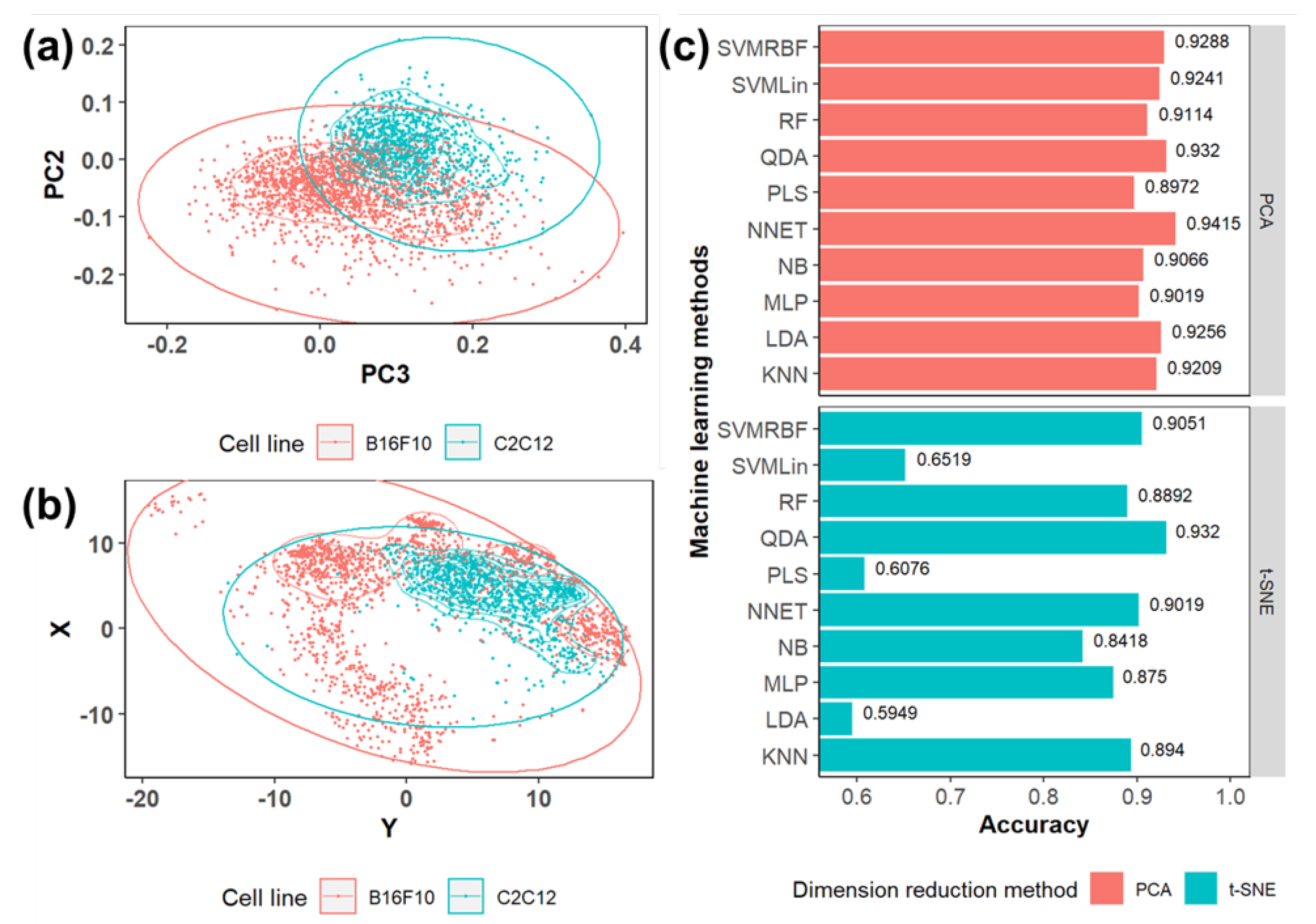
3.5. Machine Learning Classification
4. Conclusions
Supplementary Materials
Author Contributions
Funding
Institutional Review Board Statement
Informed Consent Statement
Data Availability Statement
Acknowledgments
Conflicts of Interest
References
- Balch, C. An analysis of prognostic factors in 8500 patients with cutaneous melanoma. In Cutaneous Melanoma; JB Lippincott: Philadelphia, PA, USA, 1992; pp. 163–187. [Google Scholar]
- Herring, C.L., Jr.; Harrelson, J.M.; Scully, S.P. Metastatic carcinoma to skeletal muscle: A report of 15 patients. Clin. Orthop. Relat. Res. 1998, 355, 272–281. [Google Scholar] [CrossRef]
- Viswanathan, N.; Khanna, A. Skeletal muscle metastasis from malignant melanoma. Br. J. Plast. Surg. 2005, 58, 855–858. [Google Scholar] [CrossRef]
- Kaur, B.; Kumar, S.; Kaushik, B.K. Recent advancements in optical biosensors for cancer detection. Biosens. Bioelectron. 2022, 197, 113805. [Google Scholar] [CrossRef]
- Mollasalehi, H.; Shajari, E. A colorimetric nano-biosensor for simultaneous detection of prevalent cancers using unamplified cell-free ribonucleic acid biomarkers. Bioorg. Chem. 2021, 107, 104605. [Google Scholar] [CrossRef]
- Singh, R.; Kumar, S.; Liu, F.Z.; Shuang, C.; Zhang, B.; Jha, R.; Kaushik, B.K. Etched multicore fiber sensor using copper oxide and gold nanoparticles decorated graphene oxide structure for cancer cells detection. Biosens. Bioelectron. 2020, 168, 112557. [Google Scholar] [CrossRef]
- Ayupova, T.; Shaimerdenova, M.; Sypabekova, M.; Vangelista, L.; Tosi, D. Picomolar detection of thrombin with fiber-optic ball resonator sensor using optical backscatter reflectometry. Optik 2021, 241, 166969. [Google Scholar] [CrossRef]
- Hlali, A.; Oueslati, A.; Zairi, H. Numerical simulation of tunable terahertz graphene-based sensor for breast tumor detection. IEEE Sens. J. 2021, 21, 9844–9851. [Google Scholar] [CrossRef]
- Won, H.J.; Robby, A.I.; Jhon, H.S.; In, I.; Ryu, J.H.; Park, S.Y. Wireless label-free electrochemical detection of cancer cells by MnO2-Decorated polymer dots. Sens. Actuators B Chem. 2020, 320, 128391. [Google Scholar] [CrossRef]
- Fan, M.; She, Q.; You, R.; Huang, Y.; Chen, J.; Su, H.; Lu, Y. “On-off” SERS sensor triggered by IDO for non-interference and ultrasensitive quantitative detection of IDO. Sens. Actuators B Chem. 2021, 344, 130166. [Google Scholar] [CrossRef]
- Samek, O.; Bernatová, S.; Dohnal, F. The potential of SERS as an AST methodology in clinical settings. Nanophotonics 2021, 10, 2537–2561. [Google Scholar] [CrossRef]
- Tong, D.; Chen, C.; Zhang, J.; Lv, G.; Zheng, X.; Zhang, Z.; Lv, X. Application of Raman spectroscopy in the detection of hepatitis B virus infection. Photodiagn. Photodyn. Ther. 2019, 28, 248–252. [Google Scholar] [CrossRef]
- Harz, M.; Kiehntopf, M.; Stöckel, S.; Rösch, P.; Straube, E.; Deufel, T.; Popp, J. Direct analysis of clinical relevant single bacterial cells from cerebrospinal fluid during bacterial meningitis by means of micro-Raman spectroscopy. J. Biophotonics 2009, 2, 70–80. [Google Scholar] [CrossRef]
- Pahlow, S.; Meisel, S.; Cialla-May, D.; Weber, K.; Rösch, P.; Popp, J. Isolation and identification of bacteria by means of Raman spectroscopy. Adv. Drug Deliv. Rev. 2015, 89, 105–120. [Google Scholar] [CrossRef]
- Wang, C.; Madiyar, F.; Yu, C.; Li, J. Detection of extremely low concentration waterborne pathogen using a multiplexing self-referencing SERS microfluidic biosensor. J. Biol. Eng. 2017, 11, 1–11. [Google Scholar] [CrossRef] [Green Version]
- Rebrošová, K.; Šiler, M.; Samek, O.; Rŭžička, F.; Bernatová, S.; Holá, V.; Ježek, J.; Zemánek, P.; Sokolová, J.; Petráš, P. Rapid identification of staphylococci by Raman spectroscopy. Sci. Rep. 2017, 7, 14846. [Google Scholar] [CrossRef] [Green Version]
- Pan, C.; Zhu, B.; Yu, C. A Dual Immunological Raman-Enabled Crosschecking Test (DIRECT) for Detection of Bacteria in Low Moisture Food. Biosensors 2020, 10, 200. [Google Scholar] [CrossRef]
- Bernatová, S.; Rebrošová, K.; Pilát, Z.; Šerỳ, M.; Gjevik, A.; Samek, O.; Ježek, J.; Šiler, M.; Kizovskỳ, M.; Klementová, T.; et al. Rapid detection of antibiotic sensitivity of Staphylococcus aureus by Raman tweezers. Eur. Phys. J. Plus 2021, 136, 233. [Google Scholar] [CrossRef]
- Arend, N.; Pittner, A.; Ramoji, A.; Mondol, A.S.; Dahms, M.; Rüger, J.; Kurzai, O.; Schie, I.W.; Bauer, M.; Popp, J.; et al. Detection and differentiation of bacterial and fungal infection of neutrophils from peripheral blood using Raman spectroscopy. Anal. Chem. 2020, 92, 10560–10568. [Google Scholar] [CrossRef]
- Auner, G.W.; Koya, S.K.; Huang, C.; Broadbent, B.; Trexler, M.; Auner, Z.; Elias, A.; Mehne, K.C.; Brusatori, M.A. Applications of Raman spectroscopy in cancer diagnosis. Cancer Metastasis Rev. 2018, 37, 691–717. [Google Scholar] [CrossRef] [Green Version]
- Rowlands, C.J.; Varma, S.; Perkins, W.; Leach, I.; Williams, H.; Notingher, I. Rapid acquisition of Raman spectral maps through minimal sampling: Applications in tissue imaging. J. Biophotonics 2012, 5, 220–229. [Google Scholar] [CrossRef]
- Hamada, K.; Fujita, K.; Smith, N.I.; Kobayashi, M.; Inouye, Y.; Kawata, S. Raman microscopy for dynamic molecular imaging of living cells. J. Biomed. Opt. 2008, 13, 044027. [Google Scholar] [CrossRef]
- He, H.; Xu, M.; Zong, C.; Zheng, P.; Luo, L.; Wang, L.; Ren, B. Speeding up the line-scan Raman imaging of living cells by deep convolutional neural network. Anal. Chem. 2019, 91, 7070–7077. [Google Scholar] [CrossRef]
- Huang, Z.; Teh, S.K.; Zheng, W.; Mo, J.; Lin, K.; Shao, X.; Ho, K.Y.; Teh, M.; Yeoh, K.G. Integrated Raman spectroscopy and trimodal wide-field imaging techniques for real-time in vivo tissue Raman measurements at endoscopy. Opt. Lett. 2009, 34, 758–760. [Google Scholar] [CrossRef]
- Freudiger, C.W.; Min, W.; Saar, B.G.; Lu, S.; Holtom, G.R.; He, C.; Tsai, J.C.; Kang, J.X.; Xie, X.S. Label-free biomedical imaging with high sensitivity by stimulated Raman scattering microscopy. Science 2008, 322, 1857–1861. [Google Scholar] [CrossRef] [Green Version]
- Freudiger, C.W.; Xie, X.S. In vivo imaging with stimulated Raman scattering microscopy. Opt. Photonics News 2011, 22, 27. [Google Scholar] [CrossRef] [Green Version]
- Liu, Y.J.; Kyne, M.; Wang, C.; Yu, X.Y. Data mining in Raman imaging in a cellular biological system. Comput. Struct. Biotechnol. J. 2020, 18, 2920–2930. [Google Scholar] [CrossRef]
- Guo, S.; Popp, J.; Bocklitz, T. Chemometric analysis in Raman spectroscopy from experimental design to machine learning–based modeling. Nat. Protoc. 2021, 16, 5426–5459. [Google Scholar] [CrossRef]
- Doherty, T.; McKeever, S.; Al-Attar, N.; Murphy, T.; Aura, C.; Rahman, A.; O’Neill, A.; Finn, S.P.; Kay, E.; Gallagher, W.M.; et al. Feature fusion of Raman chemical imaging and digital histopathology using machine learning for prostate cancer detection. Analyst 2021, 146, 4195–4211. [Google Scholar] [CrossRef]
- Nair, S.; Gao, J.; Yao, Q.; Duits, M.H.; Otto, C.; Mugele, F. Algorithm-improved high-speed and non-invasive confocal Raman imaging of 2D materials. Natl. Sci. Rev. 2020, 7, 620–628. [Google Scholar] [CrossRef] [Green Version]
- Perera, P.N.; Schmidt, M.; Schuck, P.J.; Adams, P.D. Blind image analysis for the compositional and structural characterization of plant cell walls. Anal. Chim. Acta 2011, 702, 172–177. [Google Scholar] [CrossRef]
- Mika, S.; Schölkopf, B.; Smola, A.J.; Müller, K.R.; Scholz, M.; Rätsch, G. Kernel PCA and De-noising in feature spaces. In Proceedings of the Advances in Neural Information Processing Systems, Denver, CO, USA, 30 November–5 December 1998; Volume 11, pp. 536–542. [Google Scholar]
- Alickovic, E.; Subasi, A. Effect of multiscale PCA denoising in ECG beat classification for diagnosis of cardiovascular diseases. Circuits Syst. Signal Process. 2015, 34, 513–533. [Google Scholar] [CrossRef]
- He, Q.; Zabotina, O.A.; Yu, C. Principal component analysis facilitated fast and noninvasive Raman spectroscopic imaging of plant cell wall pectin distribution and interaction with enzymatic hydrolysis. J. Raman Spectrosc. 2020, 51, 2458–2467. [Google Scholar] [CrossRef]
- Fang, C.; Luo, Y.; Zhang, X.; Zhang, H.; Nolan, A.; Naidu, R. Identification and visualisation of microplastics via PCA to decode Raman spectrum matrix towards imaging. Chemosphere 2022, 286, 131736. [Google Scholar] [CrossRef]
- Van der Maaten, L.; Hinton, G. Visualizing data using t-SNE. J. Mach. Learn. Res. 2008, 9, 2579–2605. [Google Scholar]
- Boser, B.E.; Guyon, I.M.; Vapnik, V.N. A training algorithm for optimal margin classifiers. In Proceedings of the Fifth Annual Workshop on Computational Learning Theory, Pittsburgh, PA, USA, 27–29 July 1992; pp. 144–152. [Google Scholar]
- Breiman, L. Random forests. Mach. Learn. 2001, 45, 5–32. [Google Scholar] [CrossRef] [Green Version]
- Ripley, B.D. Pattern Recognition and Neural Networks; Cambridge university Press: Cambridge, UK, 2007. [Google Scholar]
- Barker, M.; Rayens, W. Partial least squares for discrimination. J. Chemom. J. Chemom. Soc. 2003, 17, 166–173. [Google Scholar] [CrossRef]
- Hornik, K.; Stinchcombe, M.; White, H. Multilayer feedforward networks are universal approximators. Neural Netw. 1989, 2, 359–366. [Google Scholar] [CrossRef]
- Brozek-Pluska, B.; Jablonska-Gajewicz, J.; Kordek, R.; Abramczyk, H. Phase transitions in oleic acid and in human breast tissue as studied by Raman spectroscopy and Raman imaging. J. Med. Chem. 2011, 54, 3386–3392. [Google Scholar] [CrossRef]
- Gajjar, K.; Heppenstall, L.D.; Pang, W.; Ashton, K.M.; Trevisan, J.; Patel, I.I.; Llabjani, V.; Stringfellow, H.F.; Martin-Hirsch, P.L.; Dawson, T.; et al. Diagnostic segregation of human brain tumours using Fourier-transform infrared and/or Raman spectroscopy coupled with discriminant analysis. Anal. Methods 2013, 5, 89–102. [Google Scholar] [CrossRef]
- Abramczyk, H.; Brozek-Pluska, B.; Surmacki, J.; Jablonska-Gajewicz, J.; Kordek, R. Raman ‘optical biopsy’of human breast cancer. Prog. Biophys. Mol. Biol. 2012, 108, 74–81. [Google Scholar] [CrossRef]
- De Gelder, J.; De Gussem, K.; Vandenabeele, P.; Moens, L. Reference database of Raman spectra of biological molecules. J. Raman Spectrosc. Int. J. Orig. Work. Asp. Raman Spectrosc. Incl. High. Order Process. Brillouin Rayleigh Scatt. 2007, 38, 1133–1147. [Google Scholar] [CrossRef]
- Parker, F.S. Applications of Infrared, Raman, and Resonance Raman Spectroscopy in Biochemistry; Springer Science & Business Media: Berlin/Heidelberg, Germany, 1983. [Google Scholar]
- Notingher, I. Raman spectroscopy cell-based biosensors. Sensors 2007, 7, 1343–1358. [Google Scholar] [CrossRef] [Green Version]
- Silveira, L., Jr.; Silveira, F.L.; Zângaro, R.A.; Pacheco, M.T.; Bodanese, B. Discriminating model for diagnosis of basal cell carcinoma and melanoma in vitro based on the Raman spectra of selected biochemicals. J. Biomed. Opt. 2012, 17, 077003. [Google Scholar] [CrossRef]
- Kneipp, J.; Schut, T.B.; Kliffen, M.; Menke-Pluijmers, M.; Puppels, G. Characterization of breast duct epithelia: A Raman spectroscopic study. Vib. Spectrosc. 2003, 32, 67–74. [Google Scholar] [CrossRef]
- Jess, P.; Garcés-Chávez, V.; Smith, D.; Mazilu, M.; Paterson, L.; Riches, A.; Herrington, C.; Sibbett, W.; Dholakia, K. Dual beam fibre trap for Raman microspectroscopy of single cells. Opt. Express 2006, 14, 5779–5791. [Google Scholar] [CrossRef]
- Abramczyk, H.; Kolodziejski, M.; Waliszewska, G. Vibrational relaxation of β-carotene in acetonitrile solution and in carrot in situ. J. Mol. Liq. 1999, 79, 223–233. [Google Scholar] [CrossRef]
- Croft, D.R.; Olson, M.F. Regulating the conversion between rounded and elongated modes of cancer cell movement. Cancer Cell 2008, 14, 349–351. [Google Scholar] [CrossRef] [Green Version]
- Wand, M.; Ripley, B. KernSmooth: Functions for Kernel Smoothing for Wand & Jones (1995). R Package Version 2.22-19. 2006. Available online: https://github.com/cran/KernSmooth/blob/2.22-19/DESCRIPTION (accessed on 15 March 2022).
- Savitzky, A.; Golay, M.J. Smoothing and differentiation of data by simplified least squares procedures. Anal. Chem. 1964, 36, 1627–1639. [Google Scholar] [CrossRef]
- Lima, A.M.F.; Daniel, C.R.; Navarro, R.S.; Bodanese, B.; Pasqualucci, C.A.; Pacheco, M.T.T.; Zângaro, R.A.; Silveira, L., Jr. Discrimination of non-melanoma skin cancer and keratosis from normal skin tissue in vivo and ex vivo by Raman spectroscopy. Vib. Spectrosc. 2019, 100, 131–141. [Google Scholar] [CrossRef]
- P Santos, I.; van Doorn, R.; Caspers, P.J.; Bakker Schut, T.C.; Barroso, E.M.; Nijsten, T.E.; Noordhoek Hegt, V.; Koljenović, S.; Puppels, G.J. Improving clinical diagnosis of early-stage cutaneous melanoma based on Raman spectroscopy. Br. J. Cancer 2018, 119, 1339–1346. [Google Scholar] [CrossRef] [Green Version]
- Feng, X.; Fox, M.C.; Reichenberg, J.S.; Lopes, F.C.; Sebastian, K.R.; Markey, M.K.; Tunnell, J.W. Biophysical basis of skin cancer margin assessment using Raman spectroscopy. Biomed. Opt. Express 2019, 10, 104–118. [Google Scholar] [CrossRef]
- He, C.; Zhu, S.; Wu, X.; Zhou, J.; Chen, Y.; Qian, X.; Ye, J. Accurate Tumor Subtype Detection with Raman Spectroscopy via Variational Autoencoder and Machine Learning. ACS Omega 2022, 7, 10458–10468. [Google Scholar] [CrossRef]
- Duraipandian, S.; Traynor, D.; Kearney, P.; Martin, C.; O’Leary, J.J.; Lyng, F.M. Raman spectroscopic detection of high-grade cervical cytology: Using morphologically normal appearing cells. Sci. Rep. 2018, 8, 15048. [Google Scholar] [CrossRef] [Green Version]
- Tipatet, K.S.; Davison-Gates, L.; Tewes, T.J.; Fiagbedzi, E.K.; Elfick, A.; Neu, B.; Downes, A. Detection of acquired radioresistance in breast cancer cell lines using Raman spectroscopy and machine learning. Analyst 2021, 146, 3709–3716. [Google Scholar] [CrossRef]


| Sample | Targeted Cancer | Acquisition Time | Accuracy | Sensitivity | Specificity | Ref |
|---|---|---|---|---|---|---|
| (s) | (%) | (%) | (%) | |||
| skin tissue | skin cancer | 20 | in vivo 93.8 | 94.1 | 93.8 | [55] |
| skin cancer | ex vivo 100 | 100 | 100 | |||
| skin tissue | skin cancer | 30 | NA | 45 | 100 | [56] |
| tissue block | skin cancer | NA | NA | 100 | 84 | [57] |
| cell culture | skin cancer | 1 | 94.15 | 94.17 | 94.09 | this work |
| cell culture | breast cancer | 200 | 100 | 100 | 100 | [60] |
| cell culture | lung cancer | 2 | 89.6 | NA | NA | [58] |
| cancer tissue | kidney cancer | 5 | 81.4 | NA | NA | |
| cell culture | cervical cancer | 60 | NA | >95 | >92 | [59] |
Publisher’s Note: MDPI stays neutral with regard to jurisdictional claims in published maps and institutional affiliations. |
© 2022 by the authors. Licensee MDPI, Basel, Switzerland. This article is an open access article distributed under the terms and conditions of the Creative Commons Attribution (CC BY) license (https://creativecommons.org/licenses/by/4.0/).
Share and Cite
He, Q.; Yang, W.; Luo, W.; Wilhelm, S.; Weng, B. Label-Free Differentiation of Cancer and Non-Cancer Cells Based on Machine-Learning-Algorithm-Assisted Fast Raman Imaging. Biosensors 2022, 12, 250. https://doi.org/10.3390/bios12040250
He Q, Yang W, Luo W, Wilhelm S, Weng B. Label-Free Differentiation of Cancer and Non-Cancer Cells Based on Machine-Learning-Algorithm-Assisted Fast Raman Imaging. Biosensors. 2022; 12(4):250. https://doi.org/10.3390/bios12040250
Chicago/Turabian StyleHe, Qing, Wen Yang, Weiquan Luo, Stefan Wilhelm, and Binbin Weng. 2022. "Label-Free Differentiation of Cancer and Non-Cancer Cells Based on Machine-Learning-Algorithm-Assisted Fast Raman Imaging" Biosensors 12, no. 4: 250. https://doi.org/10.3390/bios12040250