Vibration Analysis of Fluid Conveying Carbon Nanotubes Based on Nonlocal Timoshenko Beam Theory by Spectral Element Method

Abstract
:1. Introduction
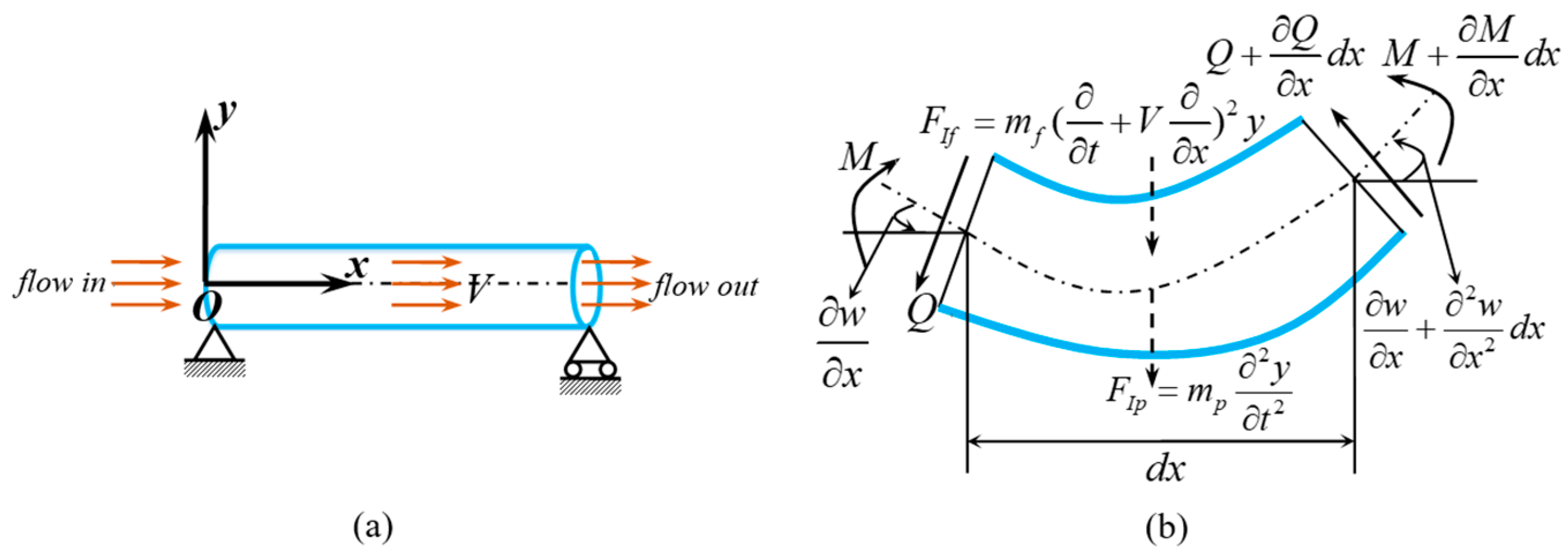
2. Dynamic Equations of SWCNT Conveying Fluid
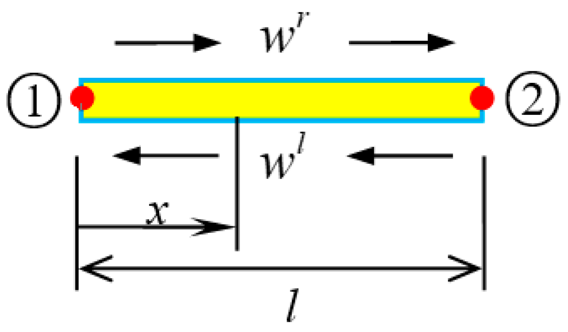
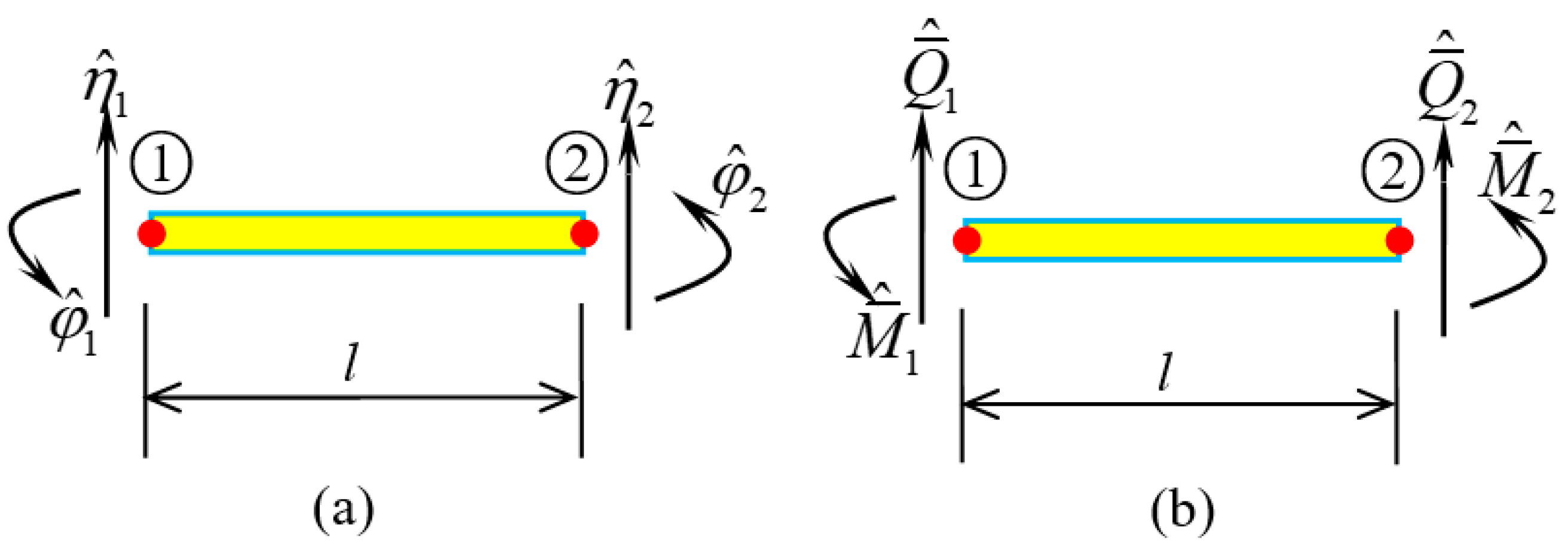
3. Spectral Formulation of a SWCNT Conveying Fluid
3.1. The Spectral Formulations
3.2. Comparison Example
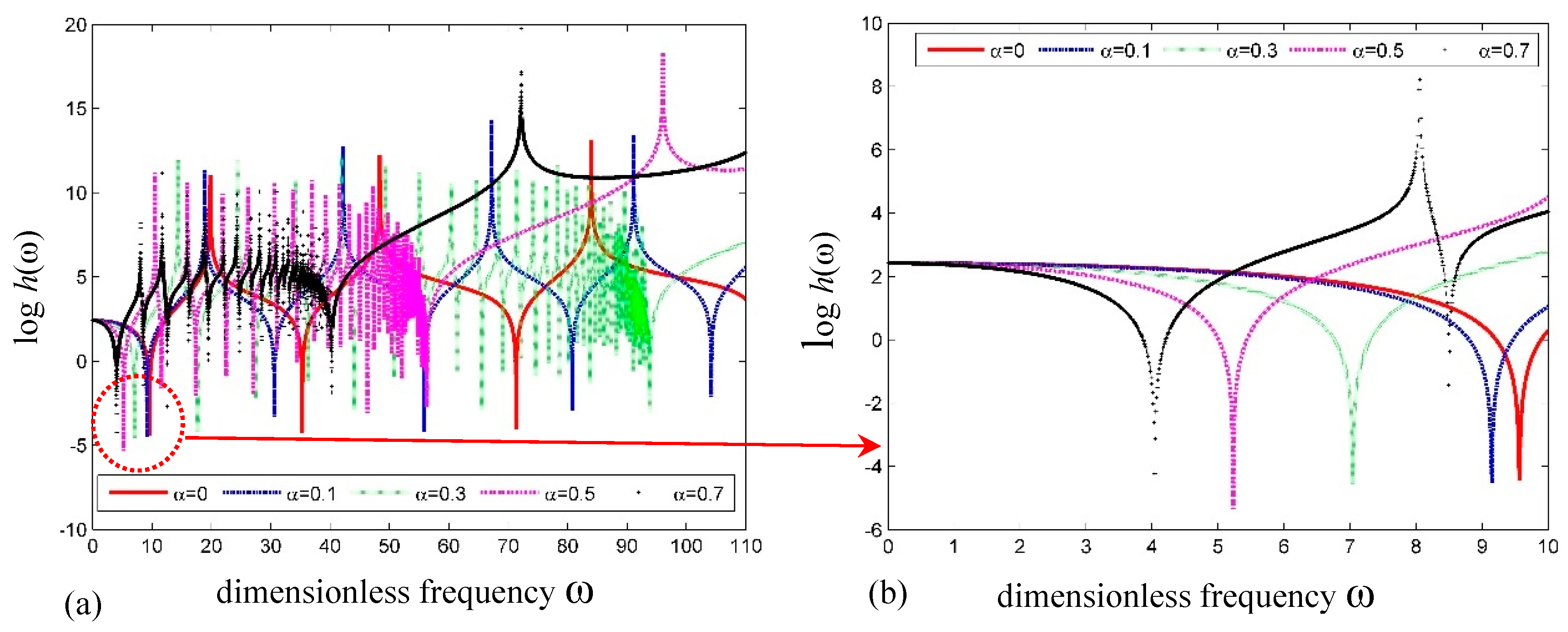
3.3. Free Vibration of a SWCNT Conveying Fluid
4. Dynamic Response of a Fluid Conveying SWCNTs
4.1. Spectral Formulations
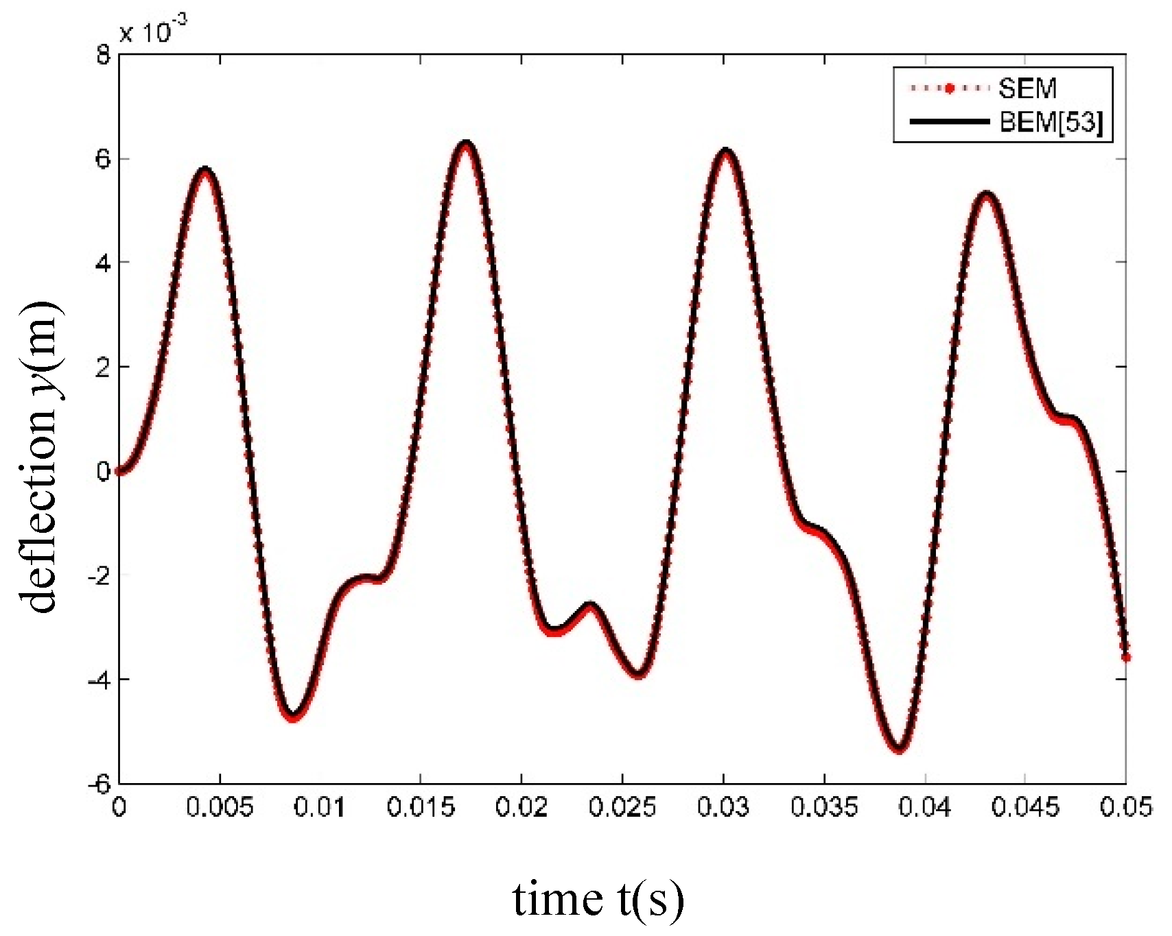
4.2. Comparison Example
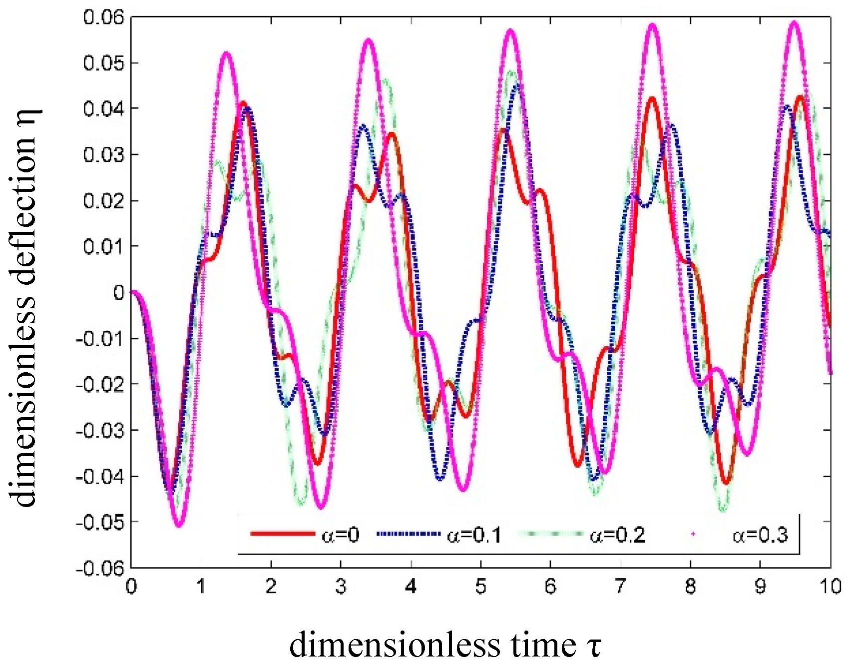
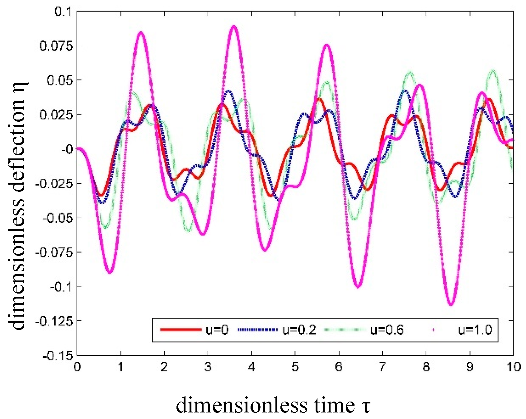
4.3. Example of SWCNT Conveying Fluid
5. Concluding Remarks
Author Contributions
Funding
Conflicts of Interest
References
- Ajayan, P.M.; Tour, J.M. Nanotube composites. Nature 2007, 447, 1066–1068. [Google Scholar] [CrossRef] [PubMed]
- Koziol, K.; Vilatela, J.; Moisala, A.; Motta, M.; Cunniff, P.; Sennett, M.; Windle, A. High-performance carbon nanotube fiber. Science 2007, 318, 1892–1895. [Google Scholar] [CrossRef] [PubMed]
- Lepak-Kuc, S.; Podsiadły, B.; Skalski, A.; Janczak, D.; Jakubowska, M.; Lekawa-Raus, A. Highly conductive carbon nanotube-thermoplastic polyurethane nanocomposite for smart clothing applications and beyond. Nanomaterials 2019, 9, 1287. [Google Scholar] [CrossRef] [PubMed] [Green Version]
- Albetran, H.; Vega, V.; Prida, V.; Low, I.M. Dynamic diffraction studies on the crystallization, phase transformation, and activation energies in anodized titania nanotubes. Nanomaterials 2018, 8, 122. [Google Scholar] [CrossRef] [PubMed] [Green Version]
- Dadrasi, A.; Albooyeh, A.R.; Mashhadzadeh, A.H. Mechanical properties of silicon-germanium nanotubes: A molecular dynamics study. Appl. Surf. Sci. 2019, 498, 143867. [Google Scholar] [CrossRef]
- Battaglia, S.; Evangelisti, S.; Leininger, T.; Pirani, F.; Faginas-Lago, N. A novel intermolecular potential to describe the interaction between the azide anion and carbon nanotubes. Diam. Relat. Mater. 2019. [Google Scholar] [CrossRef]
- Zhang, Z.; Han, S.; Wang, C.; Li, J.; Xu, G. Single-walled carbon nanohorns for energy applications. Nanomaterials 2015, 5, 1732–1755. [Google Scholar] [CrossRef] [Green Version]
- Farajpour, A.; Ghayesh, M.H.; Farokhi, H. A review on the mechanics of nanostructures. Int. J. Eng. Sci. 2018, 133, 231–263. [Google Scholar] [CrossRef]
- Ghayesh, M.H.; Farajpour, A. A review on the mechanics of functionally graded nanoscale and microscale structures. Int. J. Eng. Sci. 2019, 137, 8–36. [Google Scholar] [CrossRef]
- Li, B.; Fang, H.; He, H.; Yang, K.; Chen, C.; Wang, F. Numerical simulation and full-scale test on dynamic response of corroded concrete pipelines under multi-field coupling. Constr. Build. Mater. 2019, 200, 368–386. [Google Scholar] [CrossRef]
- Fang, H.; Lei, J.; Yang, M.; Li, Z. Analysis of GPR wave propagation using CUDA-implemented conformal symplectic partitioned Runge-Kutta method. Complexity 2019, 2019, 4025878. [Google Scholar] [CrossRef]
- Cai, K.; Yang, L.K.; Shi, J.; Qin, Q.H. Critical conditions for escape of a high-speed fullerene from a BNC nanobeam after collision. Sci. Rep. 2018, 8, 913. [Google Scholar] [CrossRef] [PubMed] [Green Version]
- Yang, L.; Cai, K.; Shi, J.; Xie, Y.M.; Qin, Q.H. Nonlinear dynamic behavior of a clamped-clamped beam from BNC nanotube impacted by fullerene. Nonlinear Dyn. 2019, 96, 1133–1145. [Google Scholar] [CrossRef]
- Ru, C.Q. Elastic models for carbon nanotubes. In Encyclopedia of Nanoscience and Nanotechnology, vol. 2; American Scientific Publishers: Stevenson Ranch, CA, USA, 2004; Volume 2, pp. 731–744. [Google Scholar]
- Eringen, A.C.; Edelen, D.G.B. On nonlocal elasticity. Int. J. Eng. Sci. 1972, 10, 233–248. [Google Scholar] [CrossRef]
- Eringen, A.C. On differential equations of nonlocal elasticity and solutions of screw dislocation and surface waves. J. Appl. Phys. 1983, 54, 4703–4710. [Google Scholar] [CrossRef]
- Lu, P.; Lee, H.P.; Lu, C. Dynamic properties of flexural beams using a nonlocal elasticity model. J. Appl. Phys. 2006, 99, 073510. [Google Scholar] [CrossRef]
- Lu, P.; Lee, H.P.; Lu, C.; Zhang, P.Q. Application of nonlocal beam models for carbon nanotubes. Int. J. Solids Struct. 2007, 44, 5289–5300. [Google Scholar] [CrossRef] [Green Version]
- Wang, C.M.; Zhang, Y.Y.; He, X.Q. Vibration of nonlocal Timoshenko beams. Nanotechnology 2007, 18, 105401. [Google Scholar] [CrossRef]
- Reddy, J.N.; Pang, S.D. Nonlocal continuum theories of beams for the analysis of carbon nanotubes. J. Appl. Phys. 2008, 103, 023511. [Google Scholar] [CrossRef]
- Reddy, J.N. Nonlocal theories for bending, buckling and vibration of beams. Int. J. Eng. Sci. 2007, 45, 288–307. [Google Scholar] [CrossRef]
- Romano, G.; Barretta, R. Nonlocal elasticity in nanobeams: The stress-driven integral model. Int. J. Eng. Sci. 2017, 115, 14–27. [Google Scholar] [CrossRef]
- Barretta, R.; Faghidian, S.A.; Sciarra, F.M. Stress-driven nonlocal integral elasticity for axisymmetric nano-plates. Int. J. Eng. Sci. 2019, 136, 38–52. [Google Scholar] [CrossRef]
- Barretta, R.; Faghidian, S.A.; Luciano, R.; Medaglia, C.M.; Penna, R. Stress-driven two-phase integral elasticity for torsion of nano-beams. Compos. Part B Eng. 2018, 145, 62–69. [Google Scholar] [CrossRef]
- Barretta, R.; Fabbrocino, F.; Luciano, R.; de Sciarra, F.M. Closed-form solutions in stress-driven two-phase integral elasticity for bending of functionally graded nano-beams. Physica E 2018, 97, 13–30. [Google Scholar] [CrossRef]
- Barretta, R.; Sciarra, F.M. Variational nonlocal gradient elasticity for nano-beams. Int. J. Eng. Sci. 2019, 143, 73–91. [Google Scholar] [CrossRef]
- Lu, L.; Guo, X.M.; Zhao, J.Z. Size-dependent vibration analysis of nanobeams based on the nonlocal strain gradient theory. Int. J. Eng. Sci. 2017, 116, 12–24. [Google Scholar] [CrossRef]
- Faghidian, S.A. Reissner stationary variational principle for nonlocal strain gradient theory of elasticity. Eur. J. Mech. A Solid 2018, 70, 115–126. [Google Scholar] [CrossRef]
- Apuzzo, A.; Barretta, R.; Faghidian, S.A.; Luciano, R.; de Sciarra, F.M. Free vibrations of elastic beams by modified nonlocal strain gradient theory. Int. J. Eng. Sci. 2018, 133, 99–108. [Google Scholar] [CrossRef]
- Hosseini, M.; Bahaadini, R. Size dependent stability analysis of cantilever micro-pipes conveying fluid based on modified strain gradient theory. Int. J. Eng. Sci. 2016, 101, 1–13. [Google Scholar] [CrossRef]
- Whitby, M.; Quirke, N. Fluid flow in carbon nanotubes and nanopipes. Nat. Nanotechnol. 2007, 2, 87–94. [Google Scholar] [CrossRef]
- Rinaldi, S.; Prabhakar, S.; Vengallatore, S.; Païdoussis, M.P. Dynamics of microscale pipes containing internal fluid flow: Damping, frequency shift, and stability. J. Sound Vib. 2010, 329, 1081–1088. [Google Scholar] [CrossRef]
- Paidoussis, M.P.; Issid, N.T. Dynamic stability of pipes conveying fluid. J. Sound Vib. 1974, 33, 267–294. [Google Scholar] [CrossRef]
- Yoon, J.; Ru, C.Q.; Mioduchowski, A. Flow-induced flutter instability of cantilever carbon nanotubes. Int. J. Solids Struct. 2006, 43, 3337–3349. [Google Scholar] [CrossRef] [Green Version]
- Yoon, J.; Ru, C.Q.; Mioduchowski, A. Vibration and instability of carbon nanotubes conveying fluid. Compos. Sci. Technol. 2005, 65, 1326–1336. [Google Scholar] [CrossRef]
- Wang, L. Size-dependent vibration characteristics of fluid-conveying microtubes. J. Fluid Struct. 2010, 26, 675–684. [Google Scholar] [CrossRef]
- Wang, L. Vibration and instability analysis of tubular nano- and micro-beams conveying fluid using nonlocal elastic theory. Phys. E 2009, 41, 1835–1840. [Google Scholar] [CrossRef]
- Wang, L. A modified nonlocal beam model for vibration and stability of nanotubes conveying fluid. Phys. E 2011, 44, 25–28. [Google Scholar] [CrossRef]
- Liang, F.; Su, Y. Stability analysis of a single-walled carbon nanotube conveying pulsating and viscous fluid with nonlocal effect. Appl. Math. Model. 2013, 37, 6821–6828. [Google Scholar] [CrossRef]
- Bahaadini, R.; Saidi, A.R.; Hosseini, M. Flow-induced vibration and stability analysis of carbon nanotubes based on the nonlocal strain gradient Timoshenko beam theory. J. Vib. Control 2018, 25, 203–218. [Google Scholar] [CrossRef]
- Afkhami, Z.; Farid, M. Thermo-mechanical vibration and instability of carbon nanocones conveying fluid using nonlocal Timoshenko beam model. J. Vib. Control 2014, 22, 604–618. [Google Scholar] [CrossRef]
- Zhen, Y.X.; Fang, B. Nonlinear vibration of fluid-conveying single-walled carbon nanotubes under harmonic excitation. Int. J. Nonlin Mech. 2015, 76, 48–55. [Google Scholar] [CrossRef]
- Ghayesh, M.H.; Farokhi, H.; Farajpour, A. Global dynamics of fluid conveying nanotubes. Int. J. Eng. Sci. 2019, 135, 37–57. [Google Scholar] [CrossRef]
- Farajpour, A.; Farokhi, H.; Ghayesh, M.H.; Hussain, S. Nonlinear mechanics of nanotubes conveying fluid. Int. J. Eng. Sci. 2018, 133, 132–143. [Google Scholar] [CrossRef]
- Doyle, J.F. Wave Propagation in Structures: An FFT-Based Spectral Analysis Methodology; Springer: Berlin/Heidelberg, Germany, 1989; p. 158. ISBN 978-1-4612-1832-6. [Google Scholar]
- Paidoussis, M.P.; Laithie, B.E. Dynamics of Timoshenko beams conveying fluid. J. Mech. Eng. Sci. 1976, 18, 210–220. [Google Scholar] [CrossRef]
- Luo, Y.; Bao, J. A material-field series-expansion method for topology optimization of continuum structures. Comput. Struct. 2019, 225, 106122. [Google Scholar] [CrossRef]
- Faghidian, S.A. Unified Formulations of the Shear Coefficients in Timoshenko Beam Theory. J. Eng. Mech. 2017, 143, 06017013. [Google Scholar] [CrossRef]
- Romano, G.; Barretta, A.; Barretta, R. On torsion and shear of Saint-Venant beams. Eur. J. Mech. A Solid 2012, 35, 47–60. [Google Scholar] [CrossRef]
- Cowper, G.R. The shear coefficient in Timoshenko’s beam theory. J. Appl. Mech. 1966, 33, 335–340. [Google Scholar] [CrossRef]
- Dym, C.L.; Shames, I.H. Solid Mechanics: A Variational Approach; Springer: Berlin/Heidelberg, Germany, 2013; p. 203. ISBN 978-1-4614-6033-6. [Google Scholar]
- Song, Y.; Kim, T.; Lee, U. Vibration of a beam subjected to a moving force: Frequency-domain spectral element modeling and analysis. Int. J. Mech. Sci. 2016, 113, 162–174. [Google Scholar] [CrossRef]
- Carrer, J.A.M.; Fleischfresser, S.A.; Garcia, L.F.T. Dynamic analysis of Timoshenko beams by the boundary element method. Eng. Anal. Bound. Elem. 2013, 37, 1602–1616. [Google Scholar] [CrossRef]


| Young’s Modulus | Diameter | Length | CNT Density | Poisson Ration | Shear Coefficient |
|---|---|---|---|---|---|
| 5.5 TPa | d = 0.678 nm | L = 10 d | 2.3 g/cm3 | μ = 0.19 | k0 = 0.563 |
| α = 0 | α = 0.1 | α = 0.3 | α = 0.5 | α = 0.7 | ||||||
|---|---|---|---|---|---|---|---|---|---|---|
| Present | [19] | Present | [19] | Present | [19] | Present | [19] | Present | [19] | |
| 3.09 | 3.09 | 3.02 | 3.02 | 2.65 | 2.65 | 2.29 | 2.29 | 2.01 | 2.01 | |
| 5.94 | 5.94 | 5.53 | 5.53 | 4.21 | 4.21 | 3.40 | 3.40 | 2.92 | 2.92 | |
| 8.44 | 8.44 | 7.47 | 7.47 | 5.24 | 5.24 | 4.16 | 4.16 | 3.55 | 3.55 | |
| 10.63 | 10.63 | 8.99 | 8.99 | 6.02 | 6.02 | 4.74 | 4.74 | 4.03 | 4.03 | |
| 12.54 | 12.54 | 10.21 | 10.21 | 6.63 | 6.63 | 5.20 | 5.20 | 4.41 | 4.41 | |
| α = 0 | α = 0.1 | α = 0.3 | α = 0.5 | |||||
|---|---|---|---|---|---|---|---|---|
| Present | [19] | Present | [19] | Present | [19] | Present | [19] | |
| 1.86 | 1.86 | 1.87 | 1.87 | 1.90 | 1.90 | 2.00 | 2.00 | |
| 4.47 | 4.47 | 4.35 | 4.35 | 3.66 | 3.66 | 2.89 | 2.89 | |
| 7.11 | 7.11 | 6.61 | 6.61 | 5.08 | 5.08 | - | - | |
| 9.38 | 9.38 | 8.32 | 8.32 | 5.79 | 5.79 | - | - | |
| 11.38 | 11.38 | 9.67 | 9.67 | 6.58 | 6.58 | - | - | |
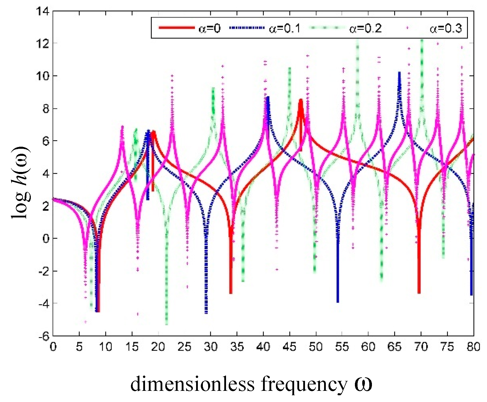
| α = 0 | α = 0.1 | α = 0.2 | α = 0.3 | |
|---|---|---|---|---|
| 8.69 | 8.26 | 7.27 | 6.14 | |
| 33.82 | 29.10 | 21.61 | 16.09 | |
| 69.61 | 54.16 | 36.12 | 25.53 | |
| 111.14 | 79.56 | 49.76 | 34.33 | |
| 155.37 | 104.07 | 62.67 | 42.53 |
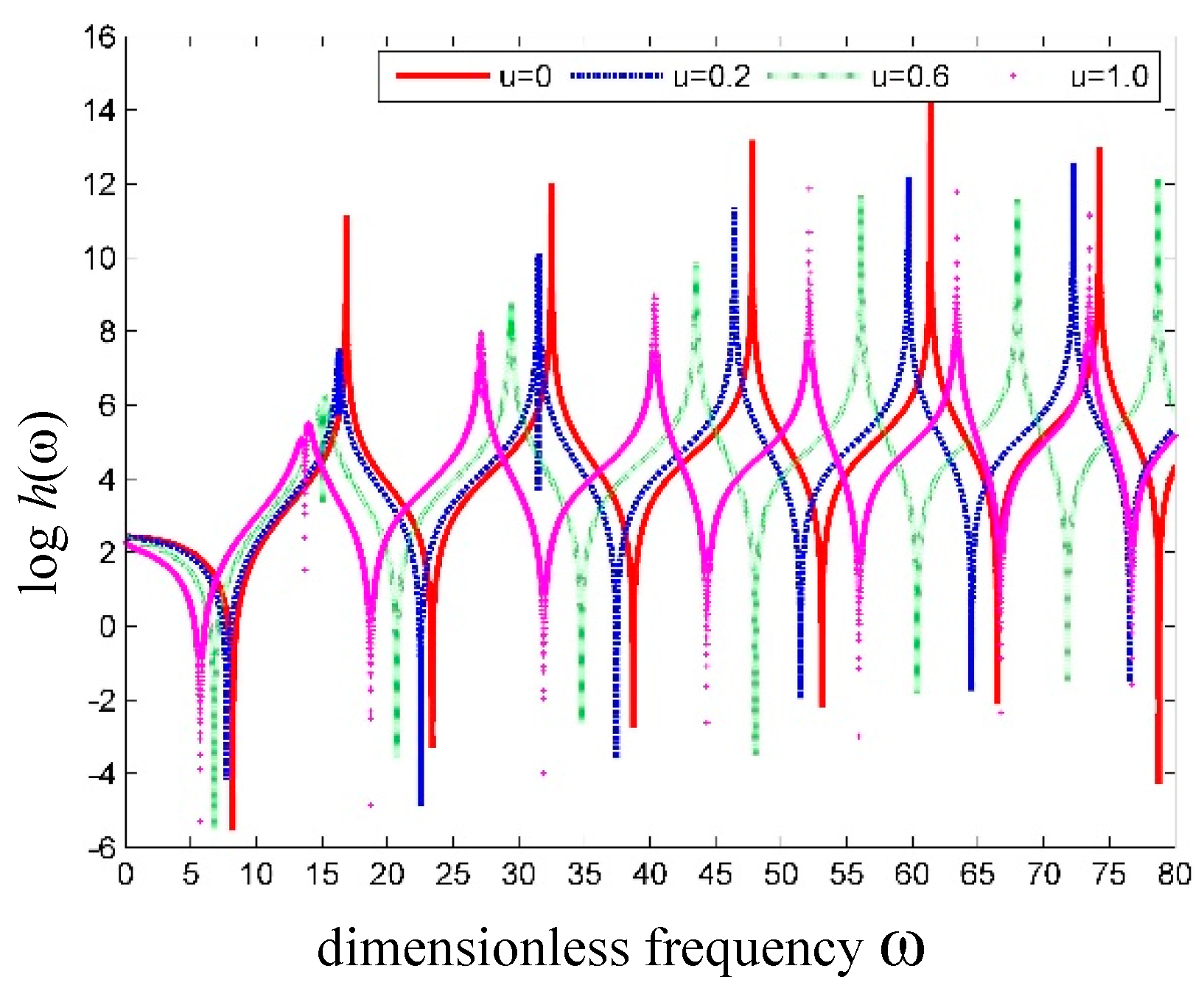
| u = 0 | u = 0.2 | u = 0.6 | u = 1.0 | |
|---|---|---|---|---|
| 8.18 | 7.74 | 6.77 | 5.70 | |
| 23.38 | 22.51 | 20.67 | 18.69 | |
| 38.69 | 37.43 | 34.76 | 31.89 | |
| 53.08 | 51.45 | 48.01 | 44.32 | |
| 66.45 | 64.50 | 60.36 | 55.92 |
| Young’s Modulus | Density | Length | Section Size | Poisson Ratio | Shear Coefficient |
|---|---|---|---|---|---|
| 50 GPa | 2.5 g/cm3 | 4 m | b = 0.2 m h = 0.6 m | μ = 0.2 | k0 = 5/6 |
© 2019 by the authors. Licensee MDPI, Basel, Switzerland. This article is an open access article distributed under the terms and conditions of the Creative Commons Attribution (CC BY) license (http://creativecommons.org/licenses/by/4.0/).
Share and Cite
Yi, X.; Li, B.; Wang, Z. Vibration Analysis of Fluid Conveying Carbon Nanotubes Based on Nonlocal Timoshenko Beam Theory by Spectral Element Method. Nanomaterials 2019, 9, 1780. https://doi.org/10.3390/nano9121780
Yi X, Li B, Wang Z. Vibration Analysis of Fluid Conveying Carbon Nanotubes Based on Nonlocal Timoshenko Beam Theory by Spectral Element Method. Nanomaterials. 2019; 9(12):1780. https://doi.org/10.3390/nano9121780
Chicago/Turabian StyleYi, Xiaolei, Baohui Li, and Zhengzhong Wang. 2019. "Vibration Analysis of Fluid Conveying Carbon Nanotubes Based on Nonlocal Timoshenko Beam Theory by Spectral Element Method" Nanomaterials 9, no. 12: 1780. https://doi.org/10.3390/nano9121780