
Active Region Overheating in Pulsed Quantum Cascade Lasers: Effects of Nonequilibrium Heat Dissipation on Laser Performance
Abstract
:1. Introduction
2. Results
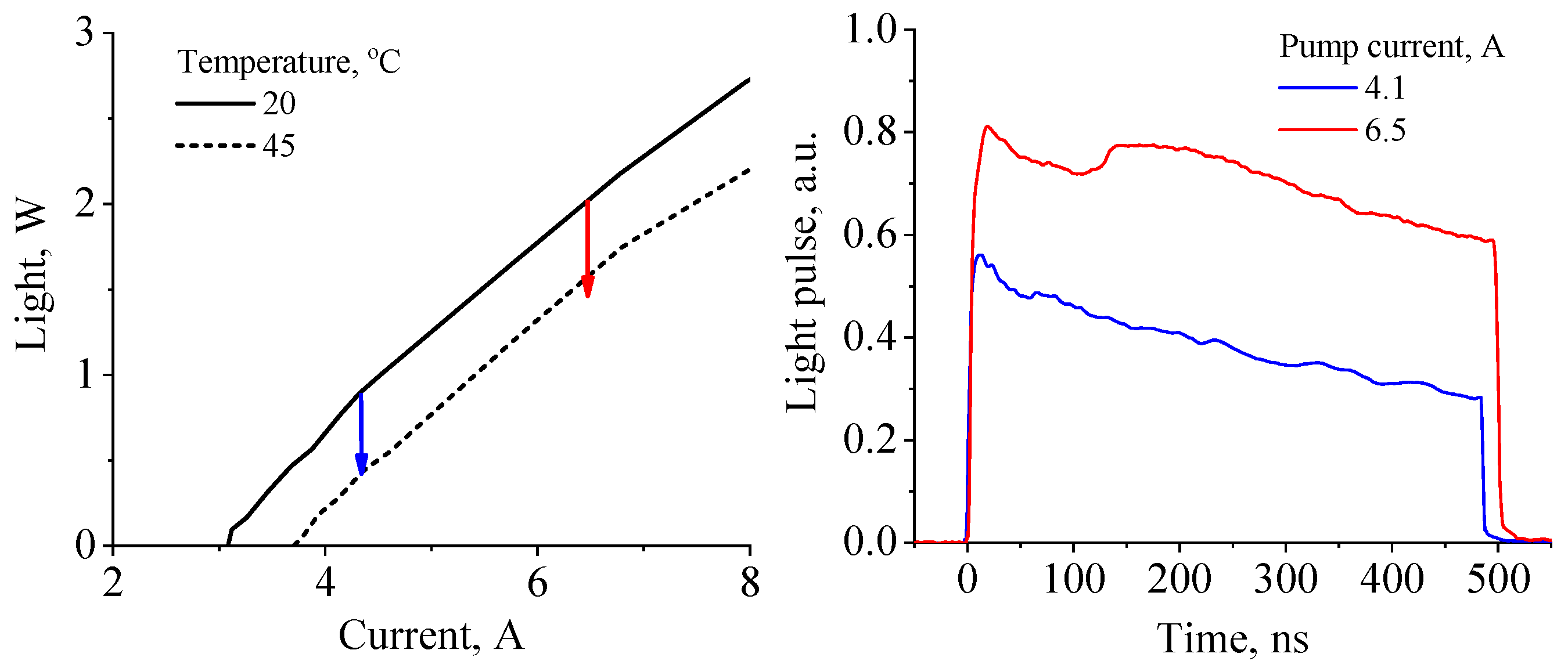
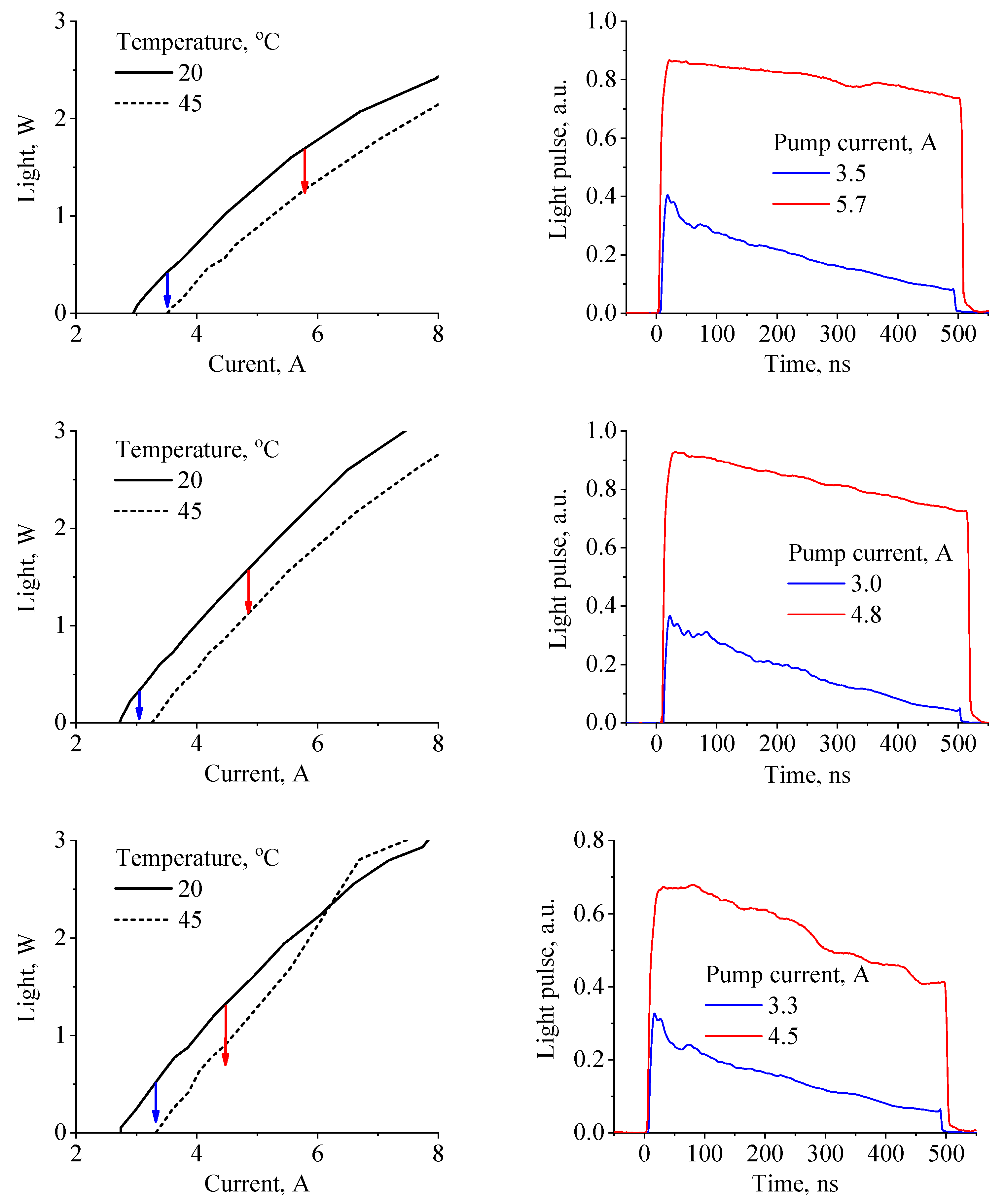
2.1. Experiment
2.2. Modeling
3. Discussion
3.1. ARn Thermal Conductivity Evaluation
3.2. Fundamental Limit on the Efficiency of Heat Transfer from ARn: Analytical Evaluation
3.3. CW Regime and Structure Safety
- The device operates at room temperature (RT);
- The temperature on the outer surface of the heat sink is stabilized equal to RT;
- The distribution of the temperature inside an ARn is neglected;
- The heat leakage from the sides of the laser ridge is neglected;
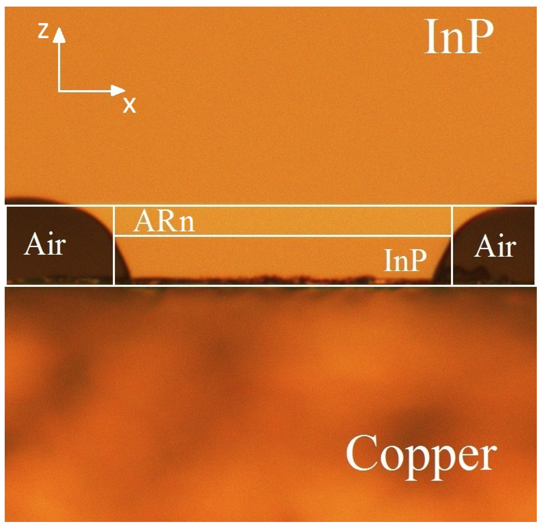
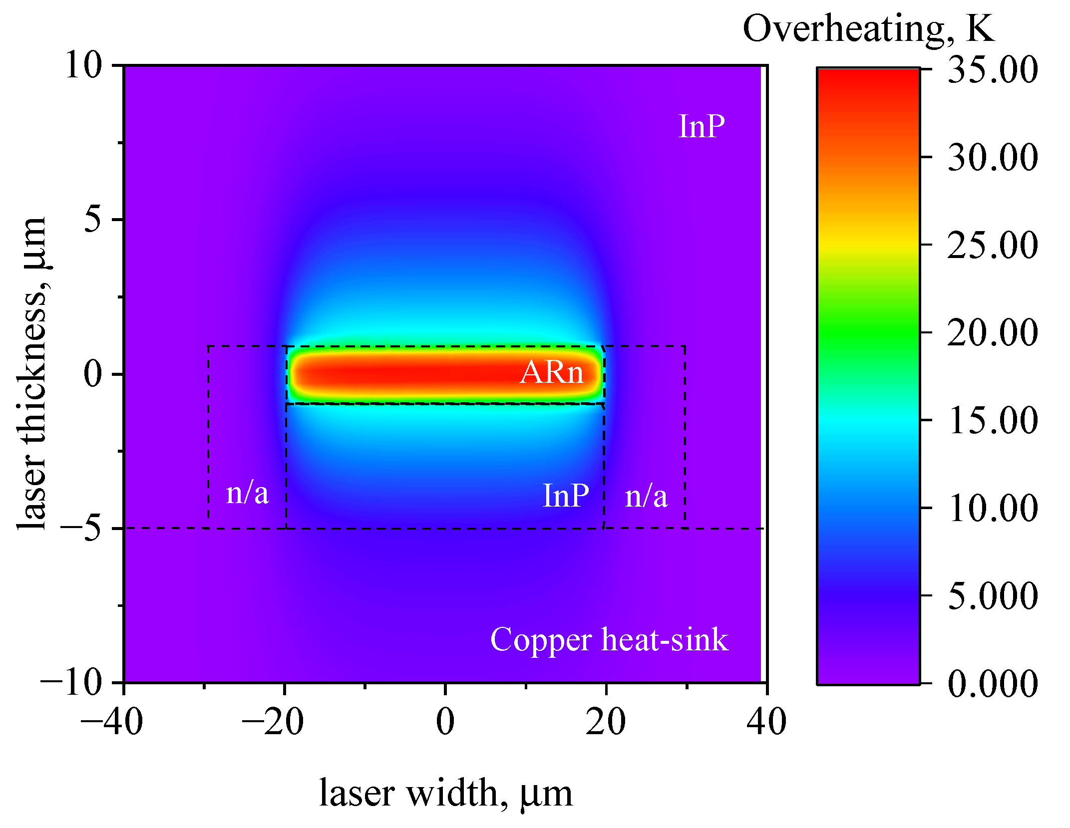
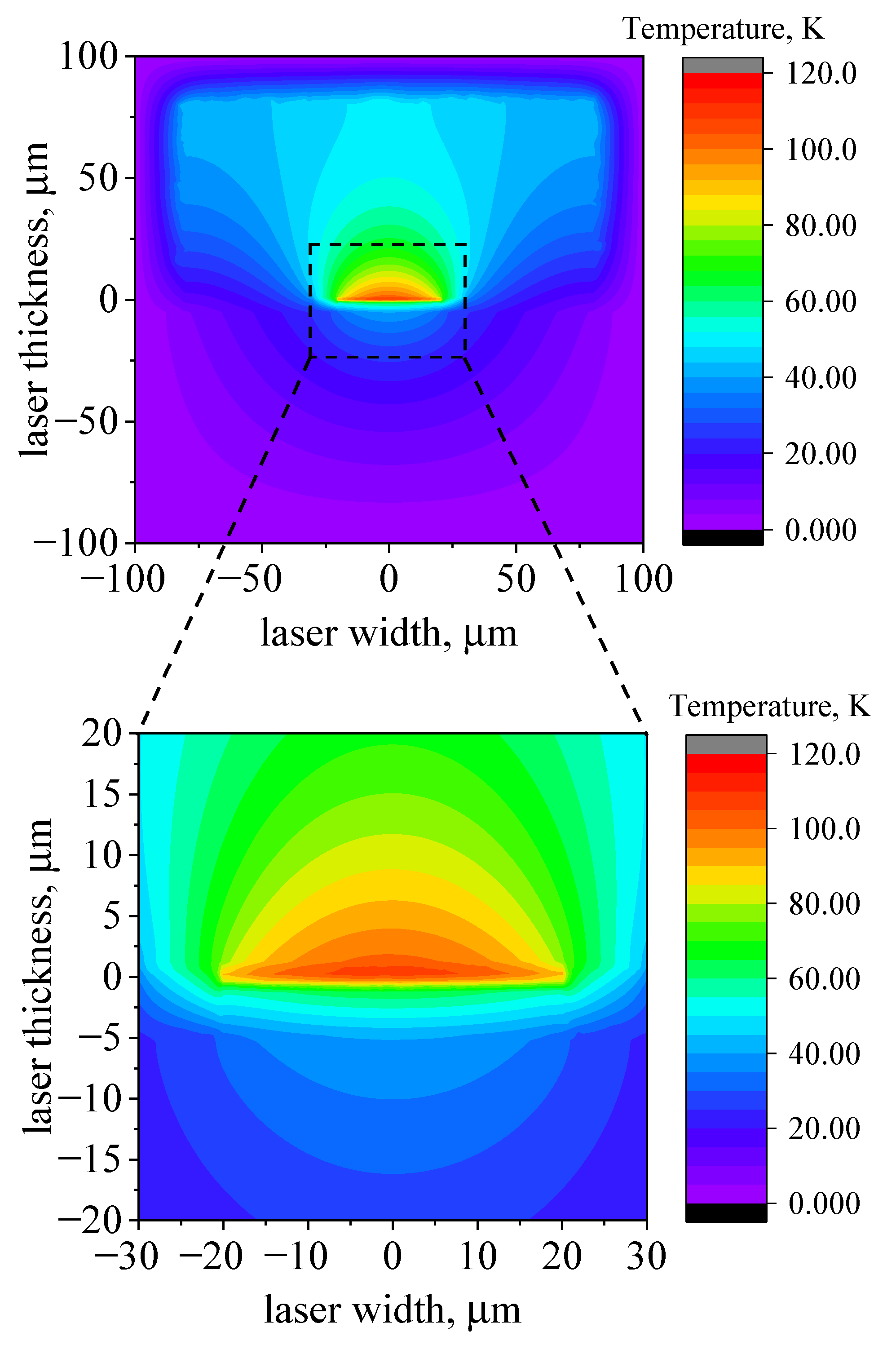
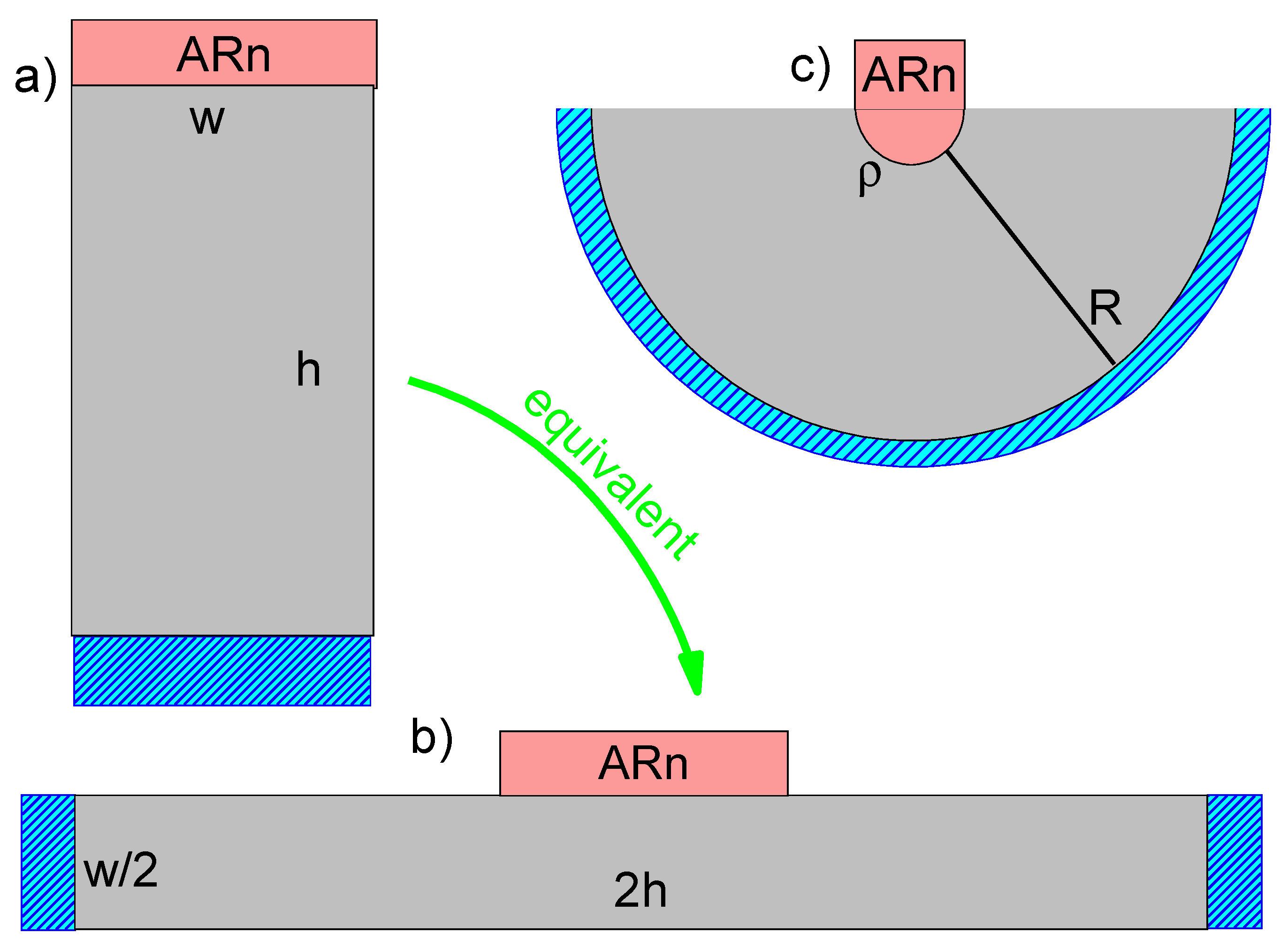
- The geometry of an ARn is needle-like, meaning that its linear dimensions in the XZ plane(facet plane) are negligible compared with the copper dimensions (see Figure 2). This allows us to consider the cylindrical distribution of isotherms in the copper heat sink. The latter agrees well with Figure 6.
4. Conclusions
Author Contributions
Funding
Data Availability Statement
Conflicts of Interest
Appendix A. Thermal Resistance of Heat Spreader Primitives

Appendix B. Other Samples

References
- Kazarinov, R.F.; Suris, R.A. Possibility of amplication of electromagnetic waves in a semiconductor with a superlattice. Sov. Phys. Semicond 1971, 5, 707–709. [Google Scholar]
- Razeghi, M.; Lu, Q.Y.; Bandyopadhyay, N.; Zhou, W.; Heydari, D.; Bai, Y.; Slivken, S. Quantum cascade lasers: From tool to product. Opt. Express 2015, 23, 8462–8475. [Google Scholar] [CrossRef] [PubMed]
- Mawst, L.J.; Botez, D. High-Power Mid-Infrared (λ 3–6 μm) Quantum Cascade Lasers. IEEE Photonics J. 2022, 14, 1–25. [Google Scholar] [CrossRef]
- Wang, F.; Slivken, S.; Wu, D.H.; Razeghi, M. Room temperature quantum cascade laser with 31% wall-plug efficiency. AIP Adv. 2020, 10, 075012. [Google Scholar] [CrossRef]
- Wang, F.; Slivken, S.; Wu, D.H.; Razeghi, M. Room temperature quantum cascade lasers with 22% wall plug efficiency in continuous-wave operation. Opt. Express 2020, 28, 17532–17538. [Google Scholar] [CrossRef]
- Wang, F.; Slivken, S.; Wu, D.H.; Lu, Q.Y.; Razeghi, M. Continuous wave quantum cascade lasers with 5.6 W output power at room temperature and 41% wall-plug efficiency in cryogenic operation. AIP Adv. 2020, 10, 055120. [Google Scholar] [CrossRef]
- Cherotchenko, E.; Dudelev, V.; Mikhailov, D.; Savchenko, G.; Chistyakov, D.; Losev, S.; Babichev, A.; Gladyshev, A.; Novikov, I.; Lutetskiy, A.; et al. High-Power Quantum Cascade Lasers Emitting at 8 μm: Technology and Analysis. Nanomaterials 2022, 12, 3971. [Google Scholar] [CrossRef]
- Faugeras, C.; Forget, S.; Boer-Duchemin, E.; Page, H.; Bengloan, J.Y.; Parillaud, O.; Calligaro, M.; Sirtori, C.; Giovannini, M.; Faist, J. High-power room temperature emission quantum cascade lasers at /spl lambda/=9 /spl mu/m. IEEE J. Quantum Electron. 2005, 41, 1430–1438. [Google Scholar] [CrossRef]
- Evans, C.; Jovanovic, V.; Indjin, D.; Ikonic, Z.; Harrison, P. Investigation of thermal effects in quantum-cascade lasers. IEEE J. Quantum Electron. 2006, 42, 859–867. [Google Scholar] [CrossRef]
- Chaparala, S.C.; Xie, F.; Caneau, C.; Zah, C.E.; Hughes, L.C. Design Guidelines for Efficient Thermal Management of Mid-Infrared Quantum Cascade Lasers. IEEE Trans. Compon. Packag. Manuf. Technol. 2011, 1, 1975–1982. [Google Scholar] [CrossRef]
- Chen, J.; Liu, Z.; Rumala, Y.; Sivco, D.; Gmachl, C.F. Direct liquid cooling of room-temperature operated quantum cascade lasers. Electron. Lett. 2006, 42, 534–535. [Google Scholar] [CrossRef]
- Wang, S. Thermal Dynamic Imaging and Thermal Management for Quantum Cascade Lasers. 2022. Available online: http://hdl.handle.net/10012/18910 (accessed on 31 October 2022).
- Pierścińska, D.; Pierściński, K.; Gutowski, P.; Badura, M.; Sobczak, G.; Serebrennikova, O.; Ściana, B.; Tłaczała, M.; Bugajski, M. Heat dissipation schemes in AlInAs/InGaAs/InP quantum cascade lasers monitored by CCD thermoreflectance. Photonics 2017, 4, 47. [Google Scholar] [CrossRef]
- Pierściński, K.; Pierścińska, D.; Iwińska, M.; Kosiel, K.; Szerling, A.; Karbownik, P.; Bugajski, M. Investigation of thermal properties of mid-infrared AlGaAs/GaAs quantum cascade lasers. J. Appl. Phys. 2012, 112, 043112. [Google Scholar] [CrossRef]
- Ladutenko, K.; Evtikhiev, V.; Revin, D.; Krysa, A. MOVPE-Grown Quantum Cascade Laser Structures Studied by Kelvin Probe Force Microscopy. Crystals 2020, 10, 129. [Google Scholar] [CrossRef]
- Babichev, A.V.; Gladyshev, A.G.; Filimonov, A.V.; Nevedomskii, V.N.; Kurochkin, A.S.; Kolodeznyi, E.S.; Sokolovskii, G.S.; Bugrov, V.E.; Karachinsky, L.Y.; Novikov, I.I.; et al. Heterostructures for quantum-cascade lasers of the wavelength range of 7–8 μm. Tech. Phys. Lett. 2017, 43, 666–669. [Google Scholar] [CrossRef]
- Howard, S.S.; Liu, Z.; Wasserman, D.; Hoffman, A.J.; Ko, T.S.; Gmachl, C.F. High-performance quantum cascade lasers: Optimized design through waveguide and thermal modeling. IEEE J. Sel. Top. Quantum Electron. 2007, 13, 1054–1064. [Google Scholar] [CrossRef]
- Babichev, A.V.; Gladyshev, A.G.; Kurochkin, A.S.; Kolodeznyi, E.S.; Sokolovskii, G.S.; Bougrov, V.; Karachinsky, L.Y.; Novikov, I.I.; Bousseksou, A.; Egorov, A.Y. Room temperature lasing of multi-stage quantum-cascade lasers at 8 μm wavelength. Semiconductors 2018, 52, 1082–1085. [Google Scholar] [CrossRef]
- Lee, H.; Yu, J. Thermal analysis of short wavelength InGaAs/InAlAs quantum cascade lasers. Solid-State Electron. 2010, 54, 769–776. [Google Scholar] [CrossRef]
- Adachi, S. Physical Properties of III-V Semiconductor Compounds; John Wiley & Sons: Hoboken, NJ, USA, 1992. [Google Scholar] [CrossRef]
- Maycock, P. Thermal conductivity of silicon, germanium, III–V compounds and III–V alloys. Solid-State Electron. 1967, 10, 161–168. [Google Scholar] [CrossRef]
- Jaffe, G.R.; Mei, S.; Boyle, C.; Kirch, J.D.; Savage, D.E.; Botez, D.; Mawst, L.J.; Knezevic, I.; Lagally, M.G.; Eriksson, M.A. Measurements of the Thermal Resistivity of InAlAs, InGaAs, and InAlAs/InGaAs Superlattices. ACS Appl. Mater. Interfaces 2019, 11, 11970–11975. [Google Scholar] [CrossRef]
- Sood, A.; Rowlette, J.A.; Caneau, C.G.; Bozorg-Grayeli, E.; Asheghi, M.; Goodson, K.E. Thermal conduction in lattice–matched superlattices of InGaAs/InAlAs. Appl. Phys. Lett. 2014, 105, 051909. [Google Scholar] [CrossRef]
- Mei, S.; Knezevic, I. Thermal conductivity of III-V semiconductor superlattices. J. Appl. Phys. 2015, 118, 175101. [Google Scholar] [CrossRef]
- Huxtable, S.T.; Shakouri, A.; Labounty, C.; Fan, X.; Abraham, P.; Chiu, Y.J.; Bowers, J.E.; Majumdar, A. Thermal Conductivity of Indium Phosphide-Based Superlattices. Microscale Thermophys. Eng. 2010, 4, 197–203. [Google Scholar] [CrossRef]
- Chen, G. Size and Interface Effects on Thermal Conductivity of Superlattices and Periodic Thin-Film Structures. J. Heat Transf. 1997, 119, 220–229. [Google Scholar] [CrossRef]
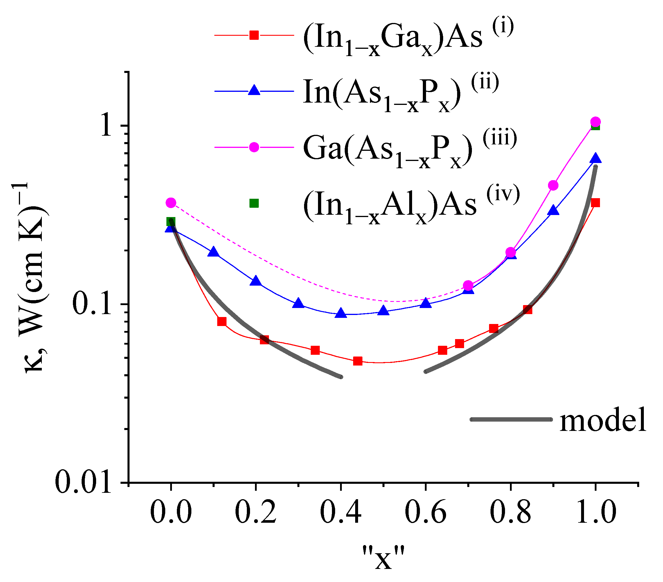
- Goryunova, N.; Kesamanly, F.; Nasledov, D. Chapter 7 Phenomena in Solid Solutions. In Semiconductors and Semimetals; Willardson, R., Beer, A.C., Eds.; Elsevier: Amsterdam, The Netherlands, 1968; Volume 4, pp. 413–458. [Google Scholar] [CrossRef]
- Afromowitz, M.A. Thermal conductivity of Ga1−xAlxAs alloys. J. Appl. Phys. 1973, 44, 1292–1294. [Google Scholar] [CrossRef]
- Abrahams, M.; Braunstein, R.; Rosi, F. Thermal, electrical and optical properties of (In,Ga)as alloys. J. Phys. Chem. Solids 1959, 10, 204–210. [Google Scholar] [CrossRef]
- Weiß, H. Thermospannung und Wärmeleitung von III—V-Verbindungen und ihren Mischkristallen. Ann. Phys. 1959, 459, 121–131. [Google Scholar] [CrossRef]
- Zhang, Q.; Liu, F.Q.; Zhang, W.; Lu, Q.; Wang, L.; Li, L.; Wang, Z. Thermal induced facet destructive feature of quantum cascade lasers. Appl. Phys. Lett. 2010, 96, 141117. [Google Scholar] [CrossRef]
- Sin, Y.; Lingley, Z.; Brodie, M.; Presser, N.; Moss, S.C.; Kirch, J.; Chang, C.C.; Boyle, C.; Mawst, L.J.; Botez, D.; et al. Destructive physical analysis of degraded quantum cascade lasers. In Proceedings of the Novel In-Plane Semiconductor Lasers XIV; Belyanin, A.A., Smowton, P.M., Eds.; International Society for Optics and Photonics, SPIE: San Francisco, CA, USA, 2015; Volume 9382, p. 93821P. [Google Scholar] [CrossRef]


| Heat Capacity, J (g K) | Density, g cm | Thermal Conductivity, W (cm·K) | |
|---|---|---|---|
| InP | 0.31 | 4.8 | 0.68 |
| Cu | 0.40 | 8.9 | 4.00 |
| ARn | 0.31 | 5.5 | 0.07 |
| Solid Solution | (), W(cm·K) | , % |
|---|---|---|
| InGaAs | 2 | 18 |
| InGaAs | 2 | 22 |
| GaAsP | 5 | 11 |
| InAsP | 1 | 30 |
| InAsP | 4 | 14 |
| Theory (InGaAs) | 4.0 (Equation (7)) | 11 (Equation (6)) |
Disclaimer/Publisher’s Note: The statements, opinions and data contained in all publications are solely those of the individual author(s) and contributor(s) and not of MDPI and/or the editor(s). MDPI and/or the editor(s) disclaim responsibility for any injury to people or property resulting from any ideas, methods, instructions or products referred to in the content. |
© 2023 by the authors. Licensee MDPI, Basel, Switzerland. This article is an open access article distributed under the terms and conditions of the Creative Commons Attribution (CC BY) license (https://creativecommons.org/licenses/by/4.0/).
Share and Cite
Vrubel, I.I.; Cherotchenko, E.D.; Mikhailov, D.A.; Chistyakov, D.V.; Abramov, A.V.; Dudelev, V.V.; Sokolovskii, G.S. Active Region Overheating in Pulsed Quantum Cascade Lasers: Effects of Nonequilibrium Heat Dissipation on Laser Performance. Nanomaterials 2023, 13, 2994. https://doi.org/10.3390/nano13232994
Vrubel II, Cherotchenko ED, Mikhailov DA, Chistyakov DV, Abramov AV, Dudelev VV, Sokolovskii GS. Active Region Overheating in Pulsed Quantum Cascade Lasers: Effects of Nonequilibrium Heat Dissipation on Laser Performance. Nanomaterials. 2023; 13(23):2994. https://doi.org/10.3390/nano13232994
Chicago/Turabian StyleVrubel, Ivan I., Evgeniia D. Cherotchenko, Dmitry A. Mikhailov, Dmitrii V. Chistyakov, Aleksandr V. Abramov, Vladislav V. Dudelev, and Grigorii S. Sokolovskii. 2023. "Active Region Overheating in Pulsed Quantum Cascade Lasers: Effects of Nonequilibrium Heat Dissipation on Laser Performance" Nanomaterials 13, no. 23: 2994. https://doi.org/10.3390/nano13232994