Nanoparticle Recognition on Scanning Probe Microscopy Images Using Computer Vision and Deep Learning

Abstract
:
1. Introduction
2. Materials and Methods
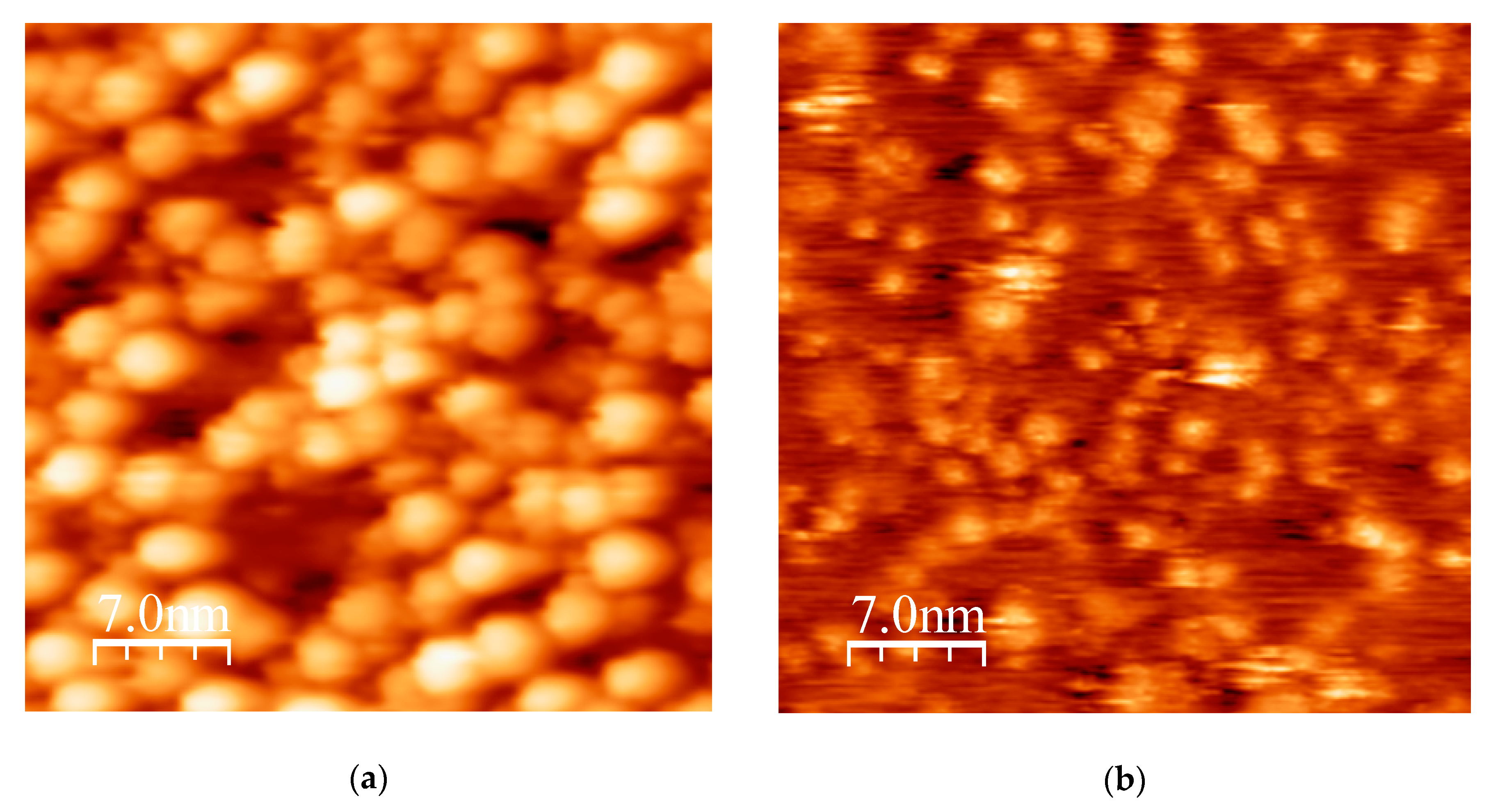
2.1. STM Data
2.2. Datasets
2.3. Neural Networks
2.4. Evaluation
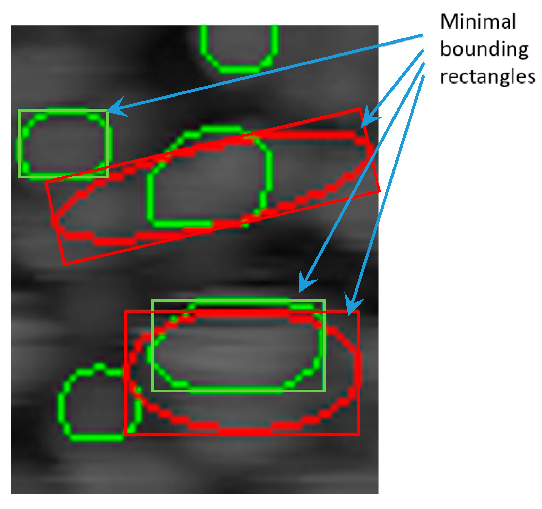
2.5. Postprocessing
3. Results
3.1. Training on a ”Rough” Dataset
3.2. Training on a ”Precise” Dataset
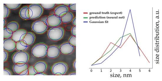
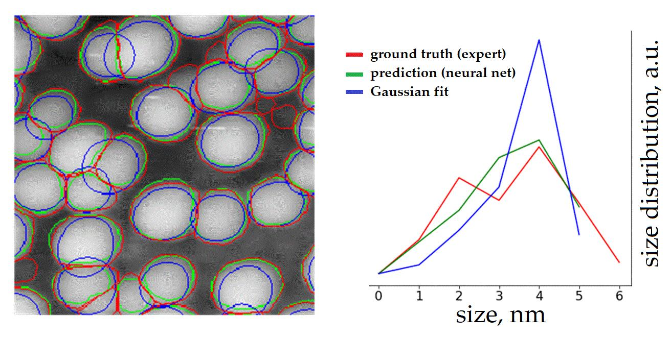
3.3. Refining Predicted Contours
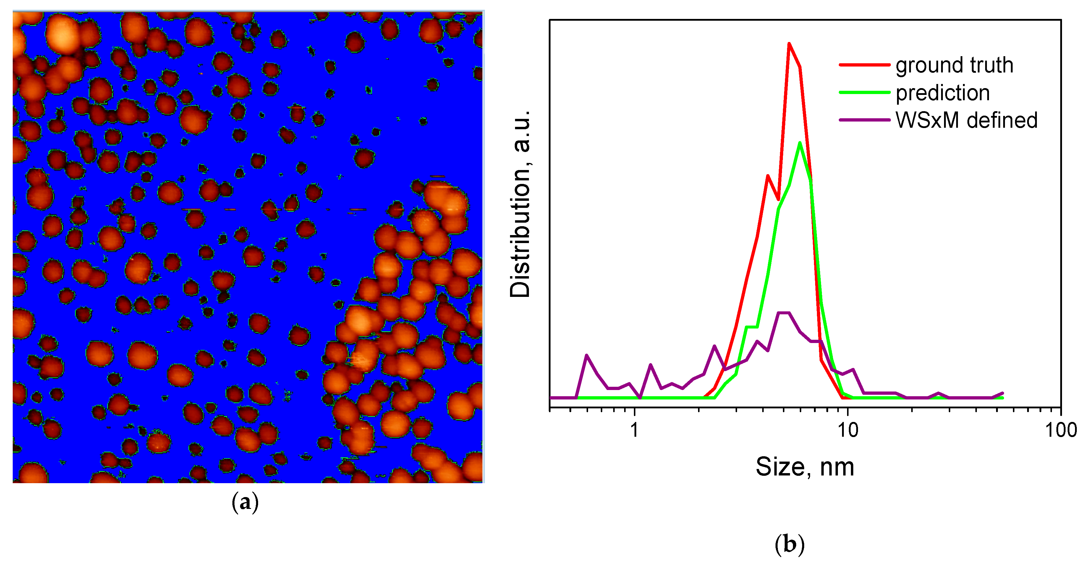
3.4. Comparison with Other Software
3.5. Online and Public Resources
4. Conclusions
- It is possible to process images containing noise, artifacts that are typical for probe microscopy images, without additional processing;
- The user can adjust automatically determined contours with the help of external software products;
- Joint statistical processing of the image sets is available;
- Processing results are displayed in the form of a histogram and tables where information on all identified objects is available.
Supplementary Materials
Author Contributions
Funding
Acknowledgments
Conflicts of Interest
References
- Nartova, A.V.; Kovtunova, L.M.; Khudorozhkov, A.K.; Shefer, K.I.; Shterk, G.V.; Kvon, R.I.; Bukhtiyarov, V.I. Influence of Preparation Conditions on Catalytic Activity and Stability of Platinum on Alumina Catalysts in Methane Oxidation. Appl. Catal. A Gen. 2018, 566, 174–180. [Google Scholar] [CrossRef]
- Smirnov, M.Y.; Vovk, E.I.; Nartova, A.V.; Kalinkin, A.V.; Bukhtiyarov, V.I. An XPS and STM Study of Oxidized Platinum Particles Formed by the Interaction between Pt/HOPG with NO2. Kinet. Catal. 2018, 59, 653–662. [Google Scholar] [CrossRef]
- Batool, M.; Hussain, D.; Akrem, A.; Najam-ul-Haq, M.; Saeed, S.; Zaka, S.M.; Nawaz, M.S.; Buck, F.; Saeed, Q. Graphene Quantum Dots as Cysteine Protease Nanocarriers Against Stored Grain Insect Pests. Sci. Rep. 2020, 10, 3444. [Google Scholar] [CrossRef] [PubMed]
- Supiandi, N.I.; Charron, G.; Tharaud, M.; Benedetti, M.F.; Sivry, Y. Tracing Multi-isotopically Labelled CdSe/ZnS Quantum Dots in Biological Media. Sci. Rep UK 2020, 10, 2866. [Google Scholar] [CrossRef] [PubMed] [Green Version]
- Bratskaya, S.; Sergeeva, K.; Konovalova, M.; Modin, E.; Svirshchevskaya, E.; Sergeev, A.; Mironenko, A.; Pestov, A. Ligand-assisted Synthesis and Cytotoxicity of ZnSe Quantum Dots Stabilized by N-(2-carboxyethyl) Chitosans. Colloids Surf. B 2019, 182, 110342. [Google Scholar] [CrossRef]
- Aleshkin, V.Y.; Baidus, N.V.; Dubinov, A.A.; Kudryavtsev, K.E.; Nekorkin, S.M.; Kruglov, A.V.; Reunov, D.G. Submonolayer InGaAs/GaAs Quantum Dots Grown by MOCVD. Semiconductors 2019, 53, 1138–1142. [Google Scholar] [CrossRef]
- Horcas, I.; Fernandez, R.; Gomez-Rodriguez, J.M.; Colchero, J.; Gomez-Herrero, J.; Baro, A.M. WSXM: A Software for Scanning Probe Microscopy and a Tool for Nanotechnology. Rev. Sci. Instrum. 2007, 78, 013705. [Google Scholar] [CrossRef]
- Gwyddion. Available online: https://sourceforge.net/projects/gwyddion/ (accessed on 1 June 2020).
- Krizhevsky, A.; Sutskever, I.; Hinton, G. Imagenet Classification with Deep Convolutional Neural Networks. In Proceedings of the Annual Conference on Neural Information Processing Systems (NIPS 2012), Lake Tahoe, NV, USA, 3–8 December 2012; pp. 1–9. [Google Scholar]
- Liu, W.; Anguelov, D.; Erhan, D.; Szegedy, C.; Reed, S.; Fu, C.-Y.; Berg, A.C. SSD: Single Shot Multibox Detector. In Computer Vision—ECCV 2016. Lecture Notes in Computer Science; Leibe, B., Matas, J., Sebe, N., Welling, M., Eds.; Springer: Cham, Switzerland, 2016; Volume 9905, pp. 21–37. [Google Scholar]
- He, K.; Gkioxari, G.; Dollar, P.; Girshick, R. Mask R-CNN. In Proceedings of the 2017 IEEE International Conference on Computer Vision (ICCV), Venice, Italy, 22–29 October 2017; pp. 2980–2988. [Google Scholar]
- Fu, G.; Sun, P.; Zhu, W.; Yang, J.; Cao, Y.; Ying-Yang, M.; Cao, Y.A. Deep-Learning-based Approach for Fast and Robust Steel Surface Defects Classification. Opt. Lasers Eng. 2019, 121, 397–405. [Google Scholar] [CrossRef]
- Zhu, H.; Ge, W.; Liu, Z. Deep Learning-Based Classification of Weld Surface Defects. Appl. Sci. 2019, 9, 3312. [Google Scholar] [CrossRef] [Green Version]
- Liu, Y.; Xu, K.; Xu, J. Periodic Surface Defect Detection in Steel Plates Based on Deep Learning. Appl. Sci. 2019, 9, 3127. [Google Scholar] [CrossRef] [Green Version]
- Feng, S.; Zhou, H.; Dong, H. Using Deep Neural Network with Small Dataset to Predict Material Defects. Mater. Des. 2019, 162, 300–310. [Google Scholar] [CrossRef]
- Yang, T.; Xiao, L.; Gong, B.; Huang, L. Surface Defect Recognition of Varistor Based on Deep Convolutional Neural Networks. In Proceedings of SPIE, Optoelectronic Imaging and Multimedia Technology VI; Dai, Q., Shimura, T., Zheng, Z., Eds.; International Society for Optics and Photonics: Bellingham, WA, USA, 2019; Volume 11187, p. 1118718. [Google Scholar]
- Ziatdinov, M.; Dyck, O.; Maksov, A.; Li, X.; Sang, X.; Xiao, K.; Unocic, R.; Vasudevan, R.; Jesse, S.; Kalinin, S.V. Deep Learning of Atomically Resolved Scanning Transmission Electron Microscopy Images: Chemical Identification and Tracking Local Transformations. ACS Nano 2017, 11, 12742–12752. [Google Scholar] [CrossRef] [PubMed] [Green Version]
- Modarres, M.H.; Aversa, R.; Cozzini, S.; Ciancio, R.; Leto, A.; Brandino, G.P. Neural Network for Nanoscience Scanning Electron Microscope Image Recognition. Sci. Rep. 2017, 7, 13282. [Google Scholar] [CrossRef] [PubMed] [Green Version]
- Poletaev, I.; Tokarev, M.P.; Pervunin, K.S. Bubble Patterns Recognition Using Neural Networks: Application to the Analysis of a Two-phase Bubbly Jet. Int. J. Multiphas Flow 2020, 126, 103194. [Google Scholar] [CrossRef]
- Qian, Y.; Huang, J.Z.; Li, X.; Ding, Y. Robust Nanoparticles Detection from Noisy Background by Fusing Complementary Image Information. IEEE Trans. Image Process. 2016, 25, 5713–5726. [Google Scholar] [CrossRef]
- Park, C.; Ding, Y. Automating material image analysis for material discovery. MRS Commun. 2019, 9, 545–555. [Google Scholar] [CrossRef] [Green Version]
- Wei, Y.; Chen, H.; Wang, H.; Wei, D.; Wu, Y.; Fan, K. Detection of Nano-particles Based on Machine Vision. In Proceedings of the 2019 IEEE International Conference on Manipulation, Manufacturing and Measurement on the Nanoscale (3M-NANO), Zhenjiang, China, 4–8 August 2019; pp. 189–192. [Google Scholar]
- Okunev, A.G.; Nartova, A.V.; Matveev, A.V. Recognition of Nanoparticles on Scanning Probe Microscopy Images Using Computer Vision and Deep Machine Learning. In Proceedings of the International Multi-Conference on Engineering, Computer and Information Sciences (SIBIRCON), Novosibirsk, Russia, 21–27 October 2019; pp. 0940–0943. [Google Scholar]
- Oktay, A.B.; Gurses, A. Automatic detection, localization and segmentation of nano-particles with deep learning in microscopy images. Micron 2019, 120, 113–119. [Google Scholar] [CrossRef]
- Zhang, F.; Zhang, Q.; Xiao, Z.; Wu, J.; Liu, Y. Spherical Nanoparticle Parameter Measurement Method based on Mask R-CNN Segmentation and Edge Fitting. In Proceedings of the 8th International Conference on Computing and Pattern Recognition (ICCPR’19), Beijing, China, 23–25 October 2019; pp. 205–212. [Google Scholar]
- Lin, T.-Y.; Maire, M.; Belongie, S.; Bourdev, L.; Girshick, R.; Hays, J.; Perona, P.; Ramanan, D.; Zitnick, C.L.; Dollár, P. Microsoft COCO: Common Objects in Context. Lect. Notes Comput. Sci. 2014, 8693, 740–755. [Google Scholar]
- Wada, K. Labelme: Image Polygonal Annotation with Python. 2016. Available online: https://github.com/wkentaro/labelme (accessed on 1 June 2020).
- Cai, Z.; Vasconcelos, N. Cascade R-CNN: Delving into High Quality Object Detection. In Proceedings of the IEEE Conference on Computer Vision and Pattern Recognition (CVPR), Salt Lake City, UT, USA, 18–22 June 2018; pp. 6154–6162. [Google Scholar]
- Everingham, M.; Van Gool, L.; Williams, C.K.I.; Winn, J.; Zisserman, A. The Pascal Visual Object Classes (voc) Challenge. Int. J. Comput. Vis. 2010, 88, 303–338. [Google Scholar] [CrossRef] [Green Version]
- COCO API-Dataset. Available online: https://github.com/cocodataset/cocoapi (accessed on 1 June 2020).
- Mukherjee, D.; Miao, L.; Stone, G.; Alem, N. Mpfit: A Robust Method for Fitting Atomic Resolution Images with Multiple Gaussian Peaks. Adv. Struct. Chem. Imag. 2020, 6, 1. [Google Scholar] [CrossRef] [Green Version]
- Anthony, S.M.; Granick, S. Image Analysis with Rapid and Accurate Two-Dimensional Gaussian Fitting. Langmuir 2009, 25, 8152–8160. [Google Scholar] [CrossRef] [PubMed]
- Yankovich, A.; Berkels, B.; Dahmen, W.; Binev, P.; Sanchez, S.I.; Bradley, S.A.; Li, A.; Szlufarska, I.; Voyles, P.M. Picometre-Precision Analysis of Scanning Transmission Electron Microscopy Images of Platinum Nanocatalysts. Nat. Commun. 2014, 5, 4155. [Google Scholar] [CrossRef] [PubMed] [Green Version]
- Wang, Y.; Salzberger, U.; Sigle, W.; Suyolcu, Y.; Van Aken, P. Oxygen Octahedra Picker: A Software Tool to Extract Quantitative Information from STEM Images. Ultramicroscopy 2016, 168, 46–52. [Google Scholar] [CrossRef] [PubMed] [Green Version]
- Web Service “ParticlesNN”. Available online: http://particlesnn.nsu.ru/ (accessed on 1 June 2020).


| No. | Backbone Type | Image Size (Rescale) | Dataset | Contours | Batch Size | Accuracy | mAP |
|---|---|---|---|---|---|---|---|
| 1 | X-101-64 × 4d-FPN | 512 × 512 (1 times) | Rough | Predicted | 12 | 0.24 | 0.000 |
| 2 | X-101-64 × 4d-FPN | 1024 × 1024 (2 times) | Rough | Predicted | 4 | 0.73 | 0.000 |
| 3 | X-101-64 × 4d-FPN | 1536 × 1536 (3 times) | Rough | Predicted | 1 | 0.83 | 0.000 |
| 4 | X-101-64 × 4d-FPN | 1536 × 1536 (3 times) | Rough | Fitted | 1 | 0.51 | 0.000 |
| 5 | HRNetV2p-W32 | 1536 × 1536 (3 times) | Rough | Predicted | 1 | 0.82 | 0.000 |
| 6 | X-101-64 × 4d-FPN | 1536 × 1536 (3 times) | Precise | Predicted | 1 | 0.78 | 0.279 |
| Image No. | Particle Count | Precision | Recall (Accuracy) | ||
|---|---|---|---|---|---|
| TP | FP | FN | |||
| 1 | 266 | 6 | 111 | 0.98 | 0.71 |
| 2 | 115 | 3 | 31 | 0.97 | 0.79 |
| 3 | 158 | 32 | 14 | 0.83 | 0.92 |
| Total | 539 | 41 | 156 | 0.93 | 0.78 |
| Backbone Type | Number of Contours Found | ||
|---|---|---|---|
| Ground Truth | Predicted | Gaussian Fitted | |
| 1 | 377 | 272 | 172 |
| 2 | 146 | 118 | 95 |
| 3 | 172 | 190 | 147 |
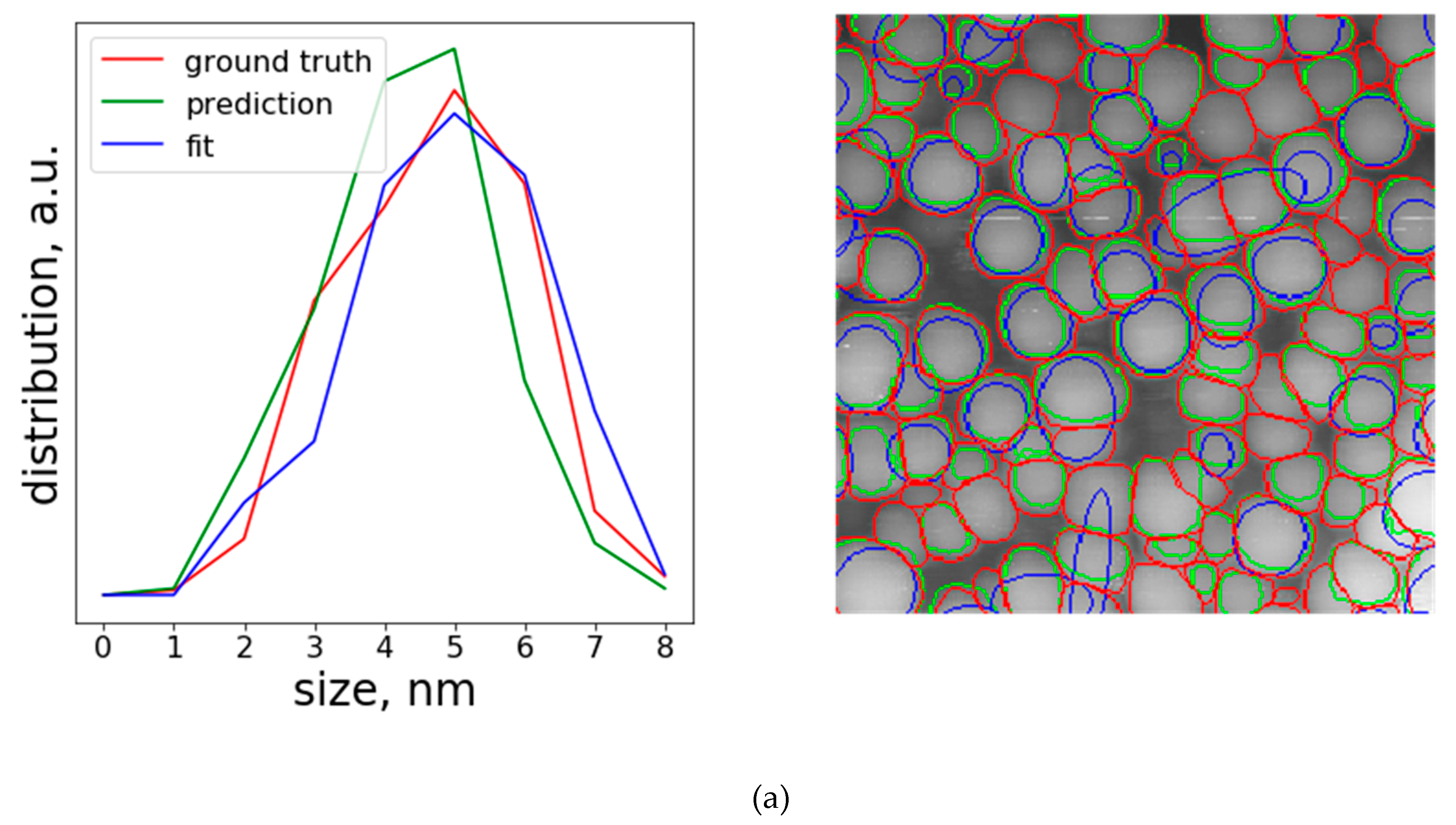
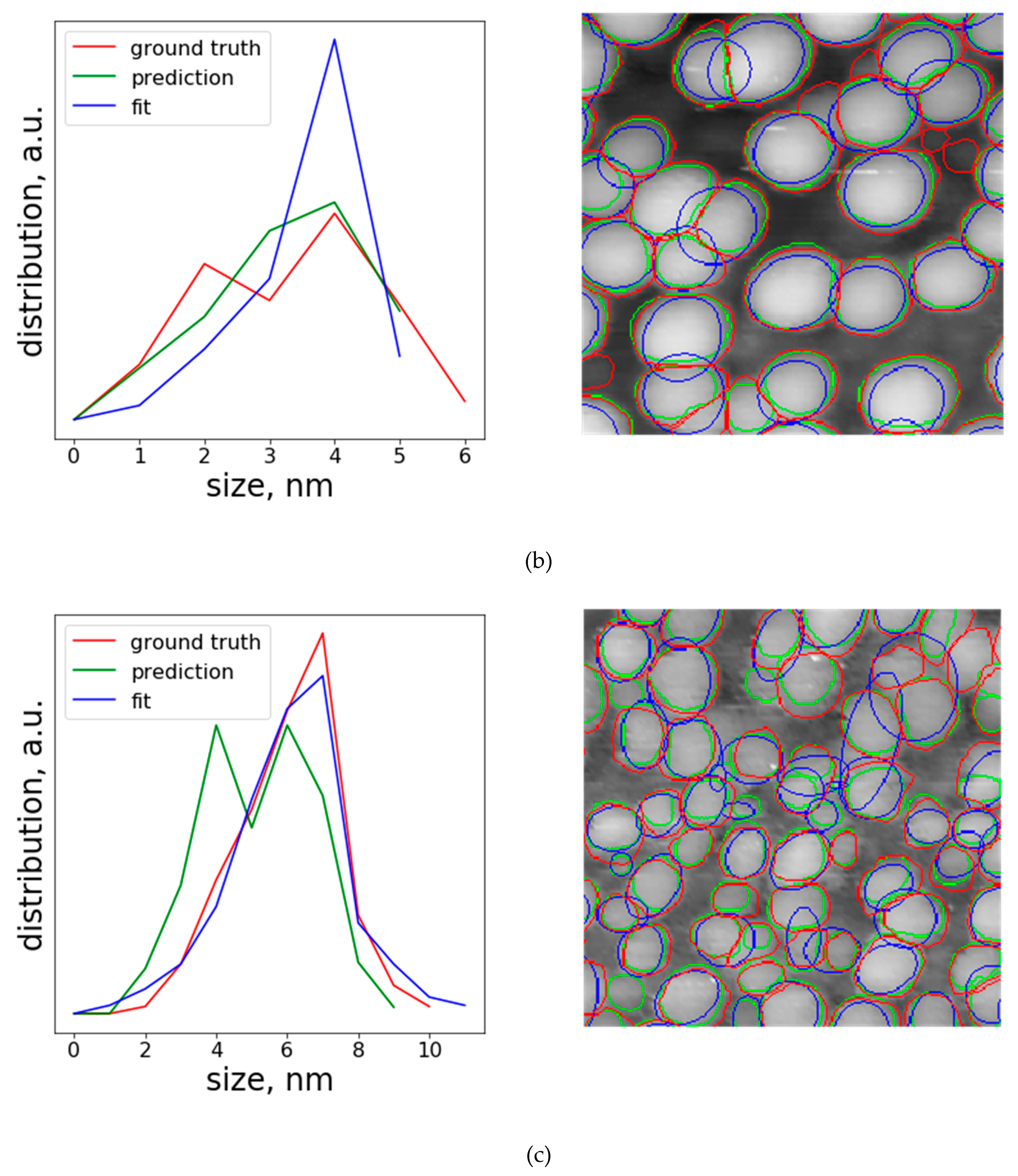
| Image No. | Mean Particle Size, nm | ||
|---|---|---|---|
| Ground Truth | Predicted | Gaussian Fitted | |
| 1 | 5.19 | 4.87 (0.94) | 5.38 (0.96) |
| 2 | 3.82 | 3.85 (0.99) | 4.15 (0.92) |
| 3 | 5.32 | 4.62 (0.87) | 5.33 (0.99) |
| Method for Determining Particle Size | Number of Particles | Mean Particle Size, nm | Standard Error of Mean |
|---|---|---|---|
| Procedure “flooding”, WSxM software | 196 1 | 4.93 1 | 0.33 1 |
| Neural network Cascade Mask-RCNN, used in this work (predicted) | 272 | 4.87 | 0.07 |
| Ground truth | 377 | 5.19 | 0.06 |
© 2020 by the authors. Licensee MDPI, Basel, Switzerland. This article is an open access article distributed under the terms and conditions of the Creative Commons Attribution (CC BY) license (http://creativecommons.org/licenses/by/4.0/).
Share and Cite
Okunev, A.G.; Mashukov, M.Y.; Nartova, A.V.; Matveev, A.V. Nanoparticle Recognition on Scanning Probe Microscopy Images Using Computer Vision and Deep Learning. Nanomaterials 2020, 10, 1285. https://doi.org/10.3390/nano10071285
Okunev AG, Mashukov MY, Nartova AV, Matveev AV. Nanoparticle Recognition on Scanning Probe Microscopy Images Using Computer Vision and Deep Learning. Nanomaterials. 2020; 10(7):1285. https://doi.org/10.3390/nano10071285
Chicago/Turabian StyleOkunev, Alexey G., Mikhail Yu. Mashukov, Anna V. Nartova, and Andrey V. Matveev. 2020. "Nanoparticle Recognition on Scanning Probe Microscopy Images Using Computer Vision and Deep Learning" Nanomaterials 10, no. 7: 1285. https://doi.org/10.3390/nano10071285