1. Introduction
The Klein–Gordon equation was discovered by several authors, including Swedish physicists Oskar Klein (1894–1977) and Walter Gordon (1893–1939) in 1926. The Klein–Gordon nonlinear equation describes various mathematical problems in engineering and science. The fractional Klein–Gordon Equation (FKGE) has important applications in relativistic physics, quantum mechanics, plasma physics, quantum field theory, nonlinear optics, solid state physics, condensed matter physics, dispersive wave phenomena and solitons. Many techniques have been implemented for solving Klein/sine–Gordon equations effectively, such as the homotopy analysis, the Adomian decomposition and the variational iteration methods [
1,
2,
3]. In this paper, a Crank–Nicolson scheme is formulated to obtain the numerical solutions of the TFKGE based on ECBS. The Caputo formula is employed for temporal discretization, while the spatial derivative is discretized using ECBS. The generalized nonlinear TFKGE is given as follows:
with the following initial conditions (ICs):
and the following boundary conditions (BCs):
where
,
are positive constants;
represents the nonlinear term;
denotes the
th order CTFD; and
is the force term.
Several analytical and numerical schemes for the TFKGE are available in the literature. In order to calculate the solutions of FKGEs, Golmankhaneh et al. [
4] employed the homotopy perturbation approach. By employing the variational iteration technique, Batiha et al. [
5] proposed an approximate solution to the sine-Gordon Equation (SGE). Kurulay [
6] presented the homotopy analysis technique to examine the nonlinear FKGEs. The Haar wavelets approach was utilized by Hariharan [
7] to solve the FKGEs. Hepson et al. [
8] proposed an exponential B-spline approach to calculate the solution of the KGE. Dehghan et al. [
9] found mathematical solutions for the fractional SGE and KGE that are nonlinear by using an implicit radial basis functions (RBFs) meshless technique. For the formulation and solution of the TFKGE, Zhang [
10] used the variational iteration approach. Chen et al. [
11] established an effective numerical spectral methodology for the nonlinear FKGEs. Nagy [
12] presented a sinc-Chebyshev collocation technique to calculate the solution of nonlinear FKGEs.
El-Sayed [
13] employed the decomposition procedure to examine the KGE. The convergence of the technique described in [
13] was examined by Kaya and El-Sayed [
14]. Cui [
15] used a compact fourth-order technique to determine the numerical solutions of the one-dimensional SGE. The homotopy analysis technique has been utilized by Jafari et al. [
16] in order to solve the nonlinear KGE. Vong and Wang [
17] provided a compact difference method for two-dimensional FKGEs involving Neumann boundaries. For the computational estimation of the Cahn–Hilliard equation and the KGE, Jafari et al. [
18] employed a fractional sub-equation approach. Mohebbi et al. [
19] used a high-order difference technique to study the linear TFKGEs. For nonlinear FKGEs, Vong and Wang [
20] established a higher-order compact approach. Recently, Yaseen et al. [
21] used the cubic trigonometric B-spline (CTBS) functions and approximated the solution of the nonlinear TFKGE. Kamran et al. [
22] approximated the solution of time fractional Phi-four equation which is a special case of the TFKGE using CBS.
An iterative scheme was used by Fang et al. [
23] to obtain the solution of the sine-Gordon and KGEs. Sweilam et al. [
24] used the Legendre pseudo spectral technique to find the numerical solution of FKGEs. Abuteen et al. [
25] proposed a numerical approach to obtain the solution of nonlinear TFKGEs by employing the reduced differential transform Scheme. To find the numerical solution of KGEs, the Taylor matrix technique was used by B
lb
l and Sezer [
26]. Hesameddini and Fotros [
27] presented the Adomian decomposition scheme to acquire the solution of the time-fractional coupled KG Schr
dinger equation. Abbasbandy [
28] presented the numerical solutions of the nonlinear KGE and nonlinear PDE with power law nonlinearities using the variation iteration technique. Singh et al. [
29] applied the homotopy perturbation technique to obtain the solution of linear and nonlinear KGEs.
The idea of splines was initially presented by Isaac Jacob Schoenberg in 1946. Carl de Boor became inspired, collaborated with Schoenberg and developed a spline recursive formula. The B-spline is widely used in engineering and mathematics. Polynomial splines are capable of approximating any continuous function over a finite interval with a high accuracy. The spline approximations were initially described by Schoenberg in [
30]. B-spline interpolation is one of the numerical methods that numerous authors have developed in recent years to solve fractional partial differential Equations (FPDEs).
In order to find numerical estimations of time FPDEs, CBS collocation methods were employed by Shafiq et al. [
31,
32]. Hepson [
33] generated the solution of the Kuramoto-Sivashinsky equation via CTBS. Yadav et al. [
34] investigated the numerical schemes with the Atangana–Baleanu derivative in two different ways and used them to obtain the solution of the advection–diffusion equation. The CBS finite element scheme was used by Majeed et al. [
35] to find the numerical solutions of time fractional fisher’s and Burgers’ equations. Mittal and Jain [
36] proposed a collocation scheme based on modified CBS to obtain the solution of the nonlinear Burgers’ equation. Tamsir et al. [
37] utilized the exponential modified CBS differential quadrature scheme to obtain the solutions of the nonlinear Burgers’ equation.
To solve FPDEs, there are several numerical approaches. One of the simplest numerical methods for estimating FPDE’s solutions at discrete points is the finite difference approach. Therefore, it has been the preference for many researchers. The fact that the problem’s solution is only determined at the selected points is a notable shortcoming in this methodology. The spline estimate approach, which yields an approximate solution in the form of an analytic curve up to a given smoothness, is used to address this limitation. As a result, approximations can be attained more accurately at any point in the domain than standard finite difference approaches. The main goal of this paper is to provide a numerical technique for the generalized nonlinear TFKGE based on ECBS. The suggested method discretizes the time-fractional derivative and the spatial derivatives using Caputo’s formula and ECBS functions, respectively. The stability of the presented scheme is established, as it is unconditionally stable. To ensure the accuracy of the scheme, a convergence analysis is discussed. To acquire the theoretical results, numerical tests are conducted and the results are compared with those that have already been provided in the literature. This technique provides more accurate results than previous studies [
19,
21,
38,
39,
40]. Furthermore, the computational errors of the proposed problem are small when they compared to other techniques. The comparison shows that our method is precise and efficient. To the best of the authors’ knowledge, the proposed method is novel and has not been previously described in the literature.
The rest of this paper is organized as follows: basic concepts are given in
Section 2. In
Section 3, the numerical technique based on ECBS functions is expounded. In
Section 4 and
Section 5, the stability and convergence of the scheme are examined, respectively. In
Section 6, our numerical findings are contrasted with those that were previously provided in [
19,
21,
38,
39,
40]. The paper concludes with some intriguing remarks, which are expressed in
Section 7.
3. Description of the Scheme
Suppose that
is partitioned into N uniform sub-intervals of size
with knots
. The ECBS functions are defined as follows [
43]:
where
,
, is serving as a free parameter and
p is a variable taking real values. For
, similar characteristics, like convex hull, geometrical invariability and symmetry, are shared by the CBS and ECBS functions. The symmetry and convex hull features guarantee the numerical stability of these functions. For
, the ECBS is reduced to the standard CBS. Let
and
be the exact and numerical solutions of Equation (
1), respectively. In terms of the above expression, the numerical solution
can be approximated as
where
are the control points. Due to the local support property of the ECBS, only
,
and
survive, so that the approximation
at the nodes
is given by
The initial and BCs are used to determine the time-dependent unknowns
. The values of
,
and
at the nodes are computed as follows:
where
,
,
,
and
.
Implementation of the Scheme
Using Equation (
3) together with the Crank–Nicolson scheme, Equation (
1) can be expressed in discretized form as
which simplifies to
where
.
It is noticed that the term
arises if
or
. To handle this term, IC is used to obtain
which reduces to
The summation term on the right-hand side of Equation (
9) can be written as
Thus, Equation (
9) becomes
For a full discretized form, we put the approximation
and its necessary derivatives (
7) into (
9) to obtain
After rearranging the above equation, it yields
This is a linear system of
equations in
unknowns. We require two additional equations, which are deducible from the provided boundary conditions to arrive at a unique solution. Thus, we have a diagonal system of dimension
, which is distinctively solvable by any appropriate numerical approach.
4. The Stability Analysis
This section demonstrates the stability of the presented scheme (
12). By utilizing the von Neumann approach, we first linearize the term
by setting
, where
is a constant [
44]. It is adequate to give the stability analysis of the suggested approach (
12) for the force-free situation
as in [
45]. The suggested scheme’s linearized form is then provided by
which reduces to
In this study, the Fourier growth factor is assumed as
, with
serving as an approximation. Define
, which, on substitution, leads to
The ICs satisfied by the above error equation are as follows:
and the boundary conditions are
Define the grid function as
The Fourier expansion for
can be expressed as
where
Let
and establish the norm
By Parseval’s equality, we have
which implies that
Assume that the solutions to Equations (
15)–(
17) are of the form
Equation (
15) can be solved by substituting the above expression as
Now, dividing the above equation by
, we obtain
Using the relation
, we obtain
Dividing the above equation by
and simplifying, we acquire
We can assume that
without losing generality. Then, the previous expression becomes
which can be written as
where
Theorem 1. If are the solutions of Equation (20), then , where . Proof. To complete the proof, we apply mathematical induction. For
, Equation (
20) becomes
with
. Now, consider
,
. Then, from Equation (
20) and using the inequality
, for
, we acquire
Theorem 2. The collocation technique (12) is unconditionally stable. Proof. Employing Theorem 1 and expression (
18), it follows that
which confirms that the scheme is unconditionally stable. □
6. Numerical Results
In this section, an approximate solution to the TFKGE (
1) is obtained by solving numerical problems. The error norms
and
are used to evaluate the scheme’s accuracy as follows:
and
Numerical computations were carried out by utilizing Mathematica 12 on an Intel(R) Core(TM) i5-3437U CPU @ 1.90 GHz (2.40 GHz Turbo), 12.0 GB RAM, an SSD, HP and a 64-bit operating system (Windows 10 Pro 10).
Example 1 ([
12]).
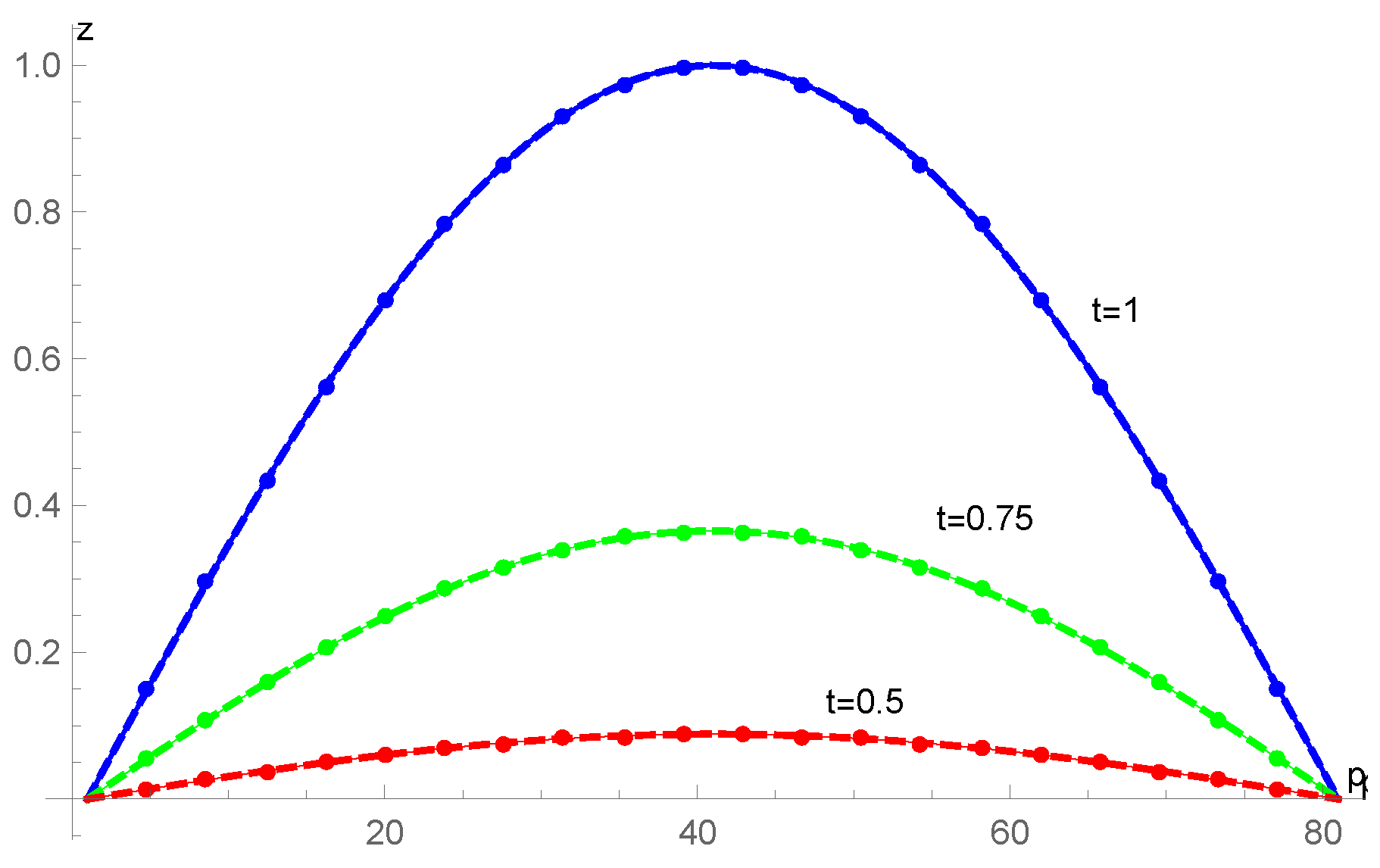
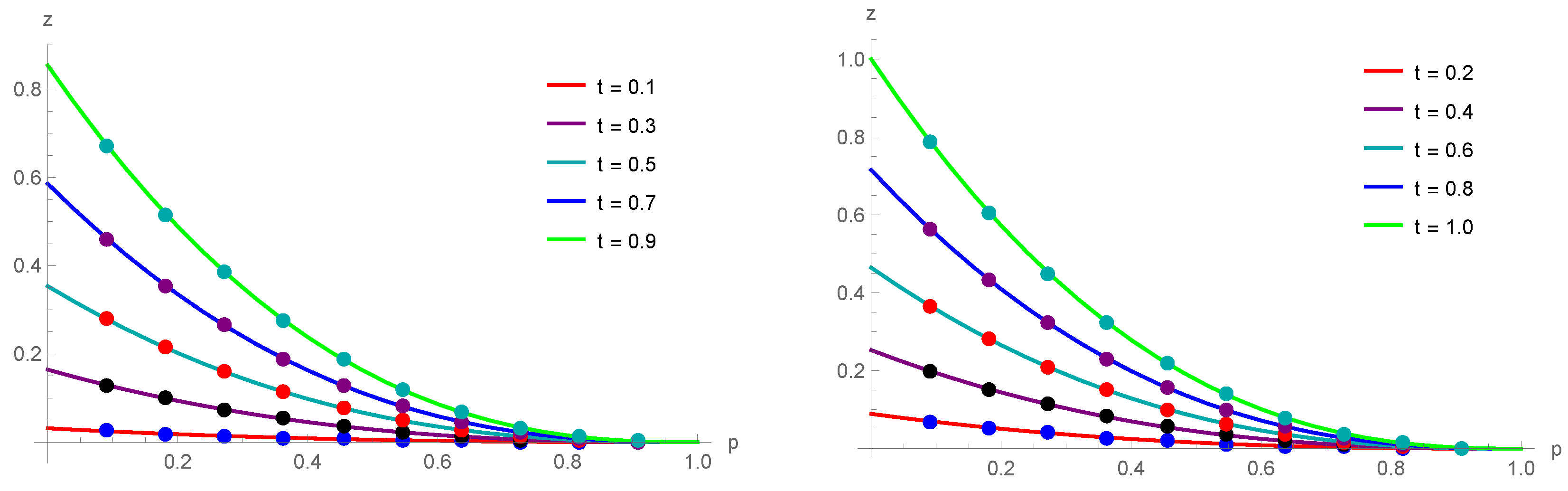
Consider the nonlinear TFKGE (1) with , , and the force term where , and is the exact solution of the given problem. The proposed approach (
12) was used to attain the numerical solution of the problem mentioned above.
Figure 1 provides a comparison of the exact and approximate solutions at various time points with
,
and
.
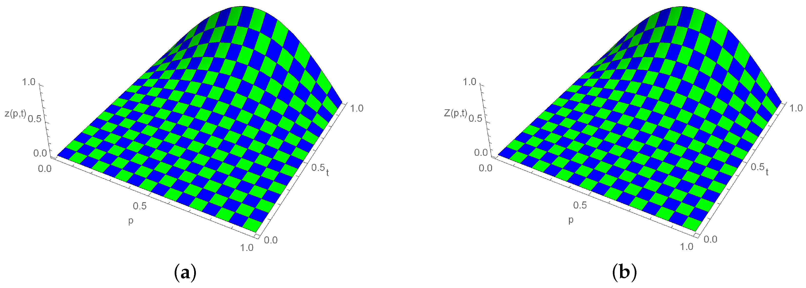
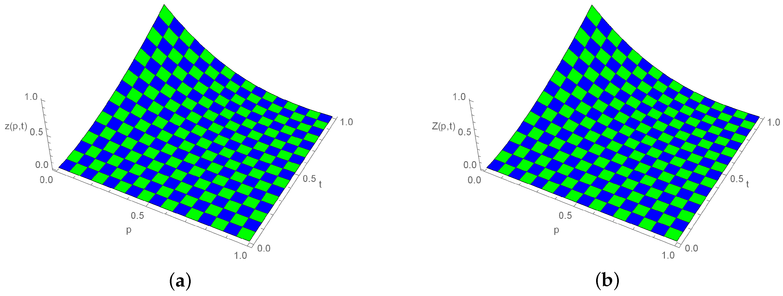
Figure 2 shows a three-dimensional (3D) comparison of the approximate (right) and exact (left) solutions. For various
values with a range of
, the absolute errors are determined and compared with the results presented in [
21] in
Table 1,
Table 2 and
Table 3. For
, the absolute errors are determined and compared with the results presented in [
38] in
Table 4. In
Table 5, for different values of
, the approximate solutions are listed.
Example 2 ([
46]).
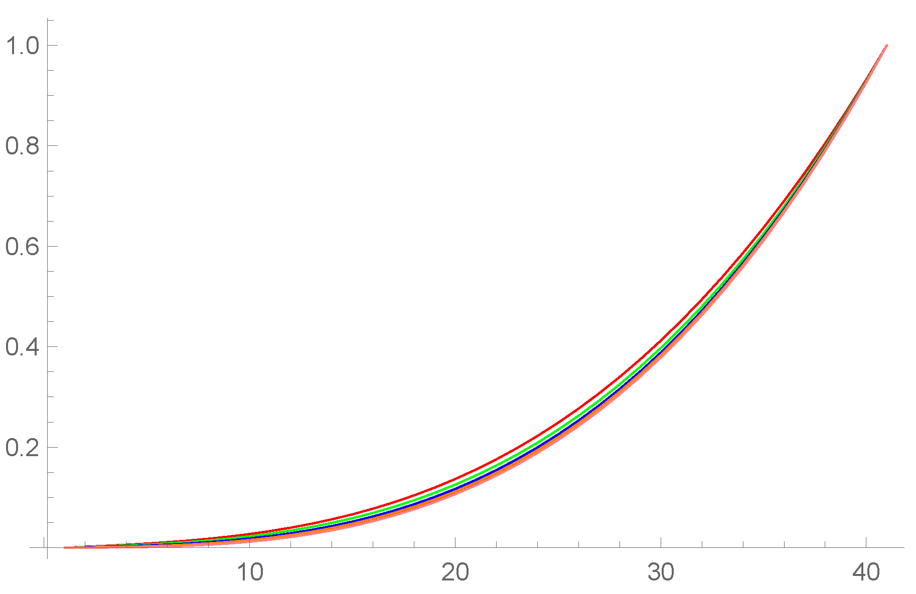
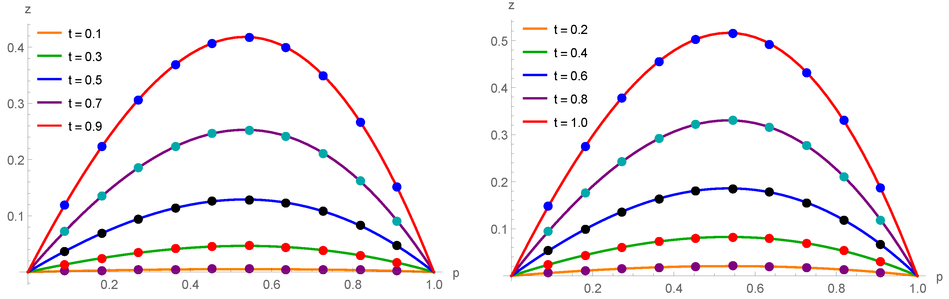
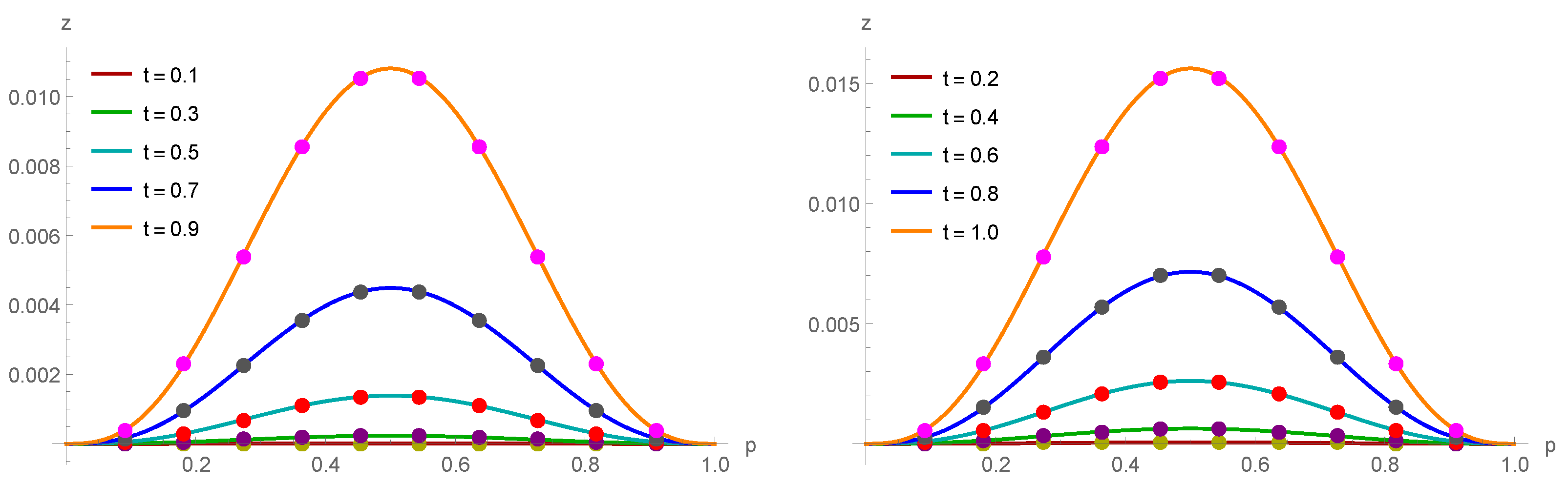
Consider the linear inhomogeneous TFKGE (1) when and The force term is The exact solution of the problem is
. Using the scheme (
12), the approximate solutions are attained for a variety of
values, and the results are shown in
Table 6. The approximate solutions for various
values of Example 2 are displayed in
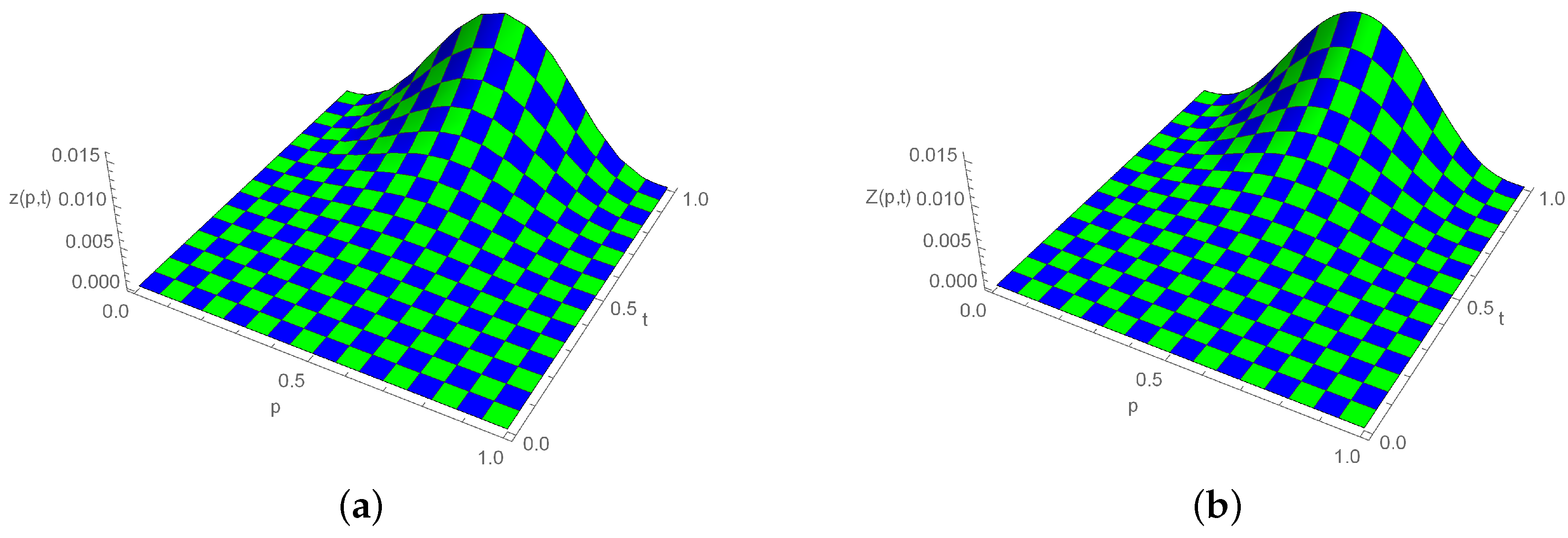
Figure 3.
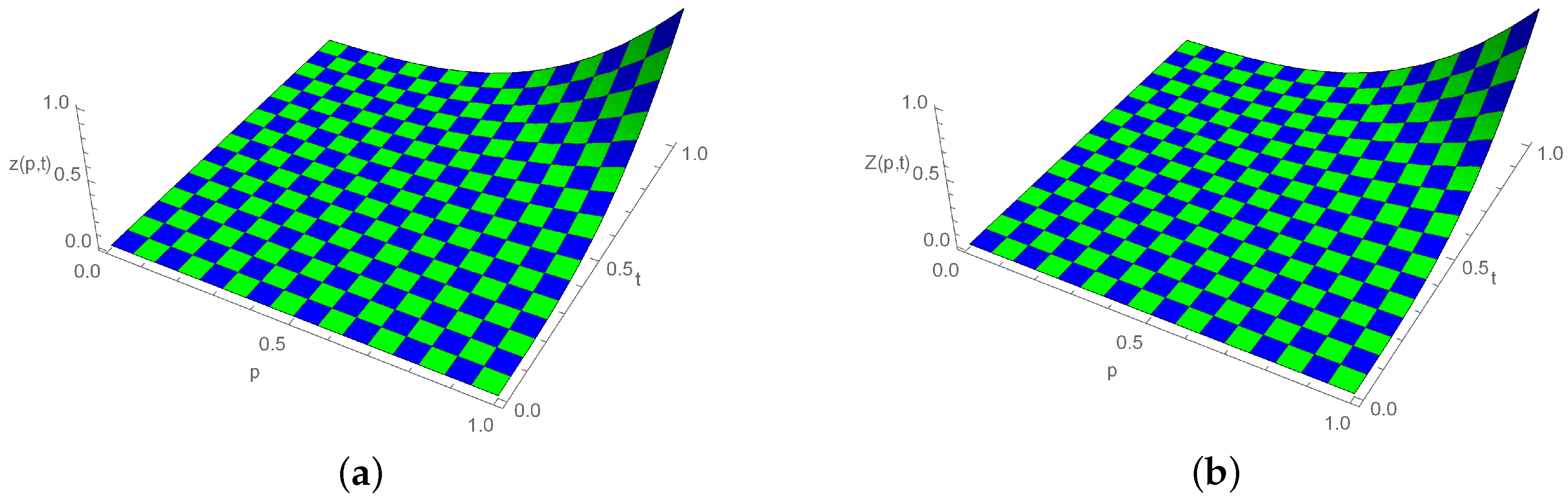
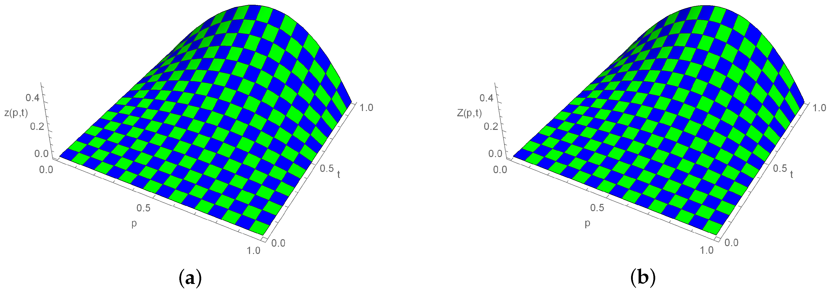
Figure 4 provides a three-dimensional (3D) comparison of exact (left) and approximate (right) solutions.
Example 3 ([
38]).
Consider the nonlinear TFKGE (1) with , , , , , , and the force term where , and is the exact solution of the given problem. Using Scheme (12), the approximate solutions were obtained, and the results are shown in Table 7. In Table 8, the comparison of error norms with [38] is listed. For , the absolute errors are determined and compared with the results presented in [38] in Table 9. Figure 5 provides a comparison of the exact and approximate solutions at various time points with , and . Figure 6 shows a three-dimensional (3D) comparison of the approximate (right) and exact (left) solutions. Example 4 ([
19,
39]).
Consider the linear TFKGE (1) with , , , , , and the force termwhere is the exact solution of the given problem. The approximate solutions are demonstrated in Table 10. In Table 11, the comparison of error norms with [19,39] is expressed. Table 12 displays the analysis of error norms in the spatial direction. Figure 7 expounds the comparison of the exact and approximate solutions at various time stages with ,
and .
Figure 8 shows a three-dimensional (3D) comparison of the approximate (right) and exact (left) solutions. Example 5 ([
40]).
Consider the nonlinear TFKGE (1) with , , , , , and the force term where , and is the exact solution of the given problem. The approximate solutions are expressed in Table 13. In Table 14 and Table 15, the comparison of error norms with [40] is demonstrated. Figure 9 represents the comparison of the exact and approximate solutions at various time stages with , and . Figure 10 expounds a three-dimensional (3D) comparison of the approximate (right) and exact (left) solutions. 


 ,
, 


