Article

Predicting Time-to-Healing from a Digital Wound Image: A Hybrid Neural Network and Decision Tree Approach Improves Performance

1
School of Electrical Engineering and Computer Science, Oregon State University, Corvallis, OR 97331, USA
2
Institute for Systems Biology, 401 Terry Ave N, Seattle, WA 98109, USA
3
Department of Biomedical Sciences, Oregon State University, Corvallis, OR 97331, USA
*
Author to whom correspondence should be addressed.
These authors contributed equally to this work.
Computation 2024, 12(3), 42; https://doi.org/10.3390/computation12030042
Submission received: 23 January 2024 / Revised: 20 February 2024 / Accepted: 23 February 2024 / Published: 28 February 2024
(This article belongs to the Special Issue Computational Medical Image Analysis)

Abstract

:

Simple Summary

In this work, we explored computational methods for analyzing a color digital image of a wound and predicting (from the analyzed image) the number of days it will take for the wound to fully heal. We used a hybrid computational approach combining deep neural networks and decision trees, and within this hybrid approach, we explored (and compared the accuracies of) different types of models for predicting the time to heal. More specifically, we explored different models for finding the outline of the wound within the wound image and we proposed a model for computing the proportions of different types of tissues within the wound bed (e.g., fibrin slough, granulation, or necrotic tissue). Our work clarifies what type of model should be used for the computational prediction of wound time-to-healing and establishes that, in order to predict time-to-healing accurately, it is important to incorporate (into the model) data on the proportions of different types in the wound bed.

Abstract

Despite the societal burden of chronic wounds and despite advances in image processing, automated image-based prediction of wound prognosis is not yet in routine clinical practice. While specific tissue types are known to be positive or negative prognostic indicators, image-based wound healing prediction systems that have been demonstrated to date do not (1) use information about the proportions of tissue types within the wound and (2) predict time-to-healing (most predict categorical clinical labels). In this work, we analyzed a unique dataset of time-series images of healing wounds from a controlled study in dogs, as well as human wound images that are annotated for the tissue type composition. In the context of a hybrid-learning approach (neural network segmentation and decision tree regression) for the image-based prediction of time-to-healing, we tested whether explicitly incorporating tissue type-derived features into the model would improve the accuracy for time-to-healing prediction versus not including such features. We tested four deep convolutional encoder–decoder neural network models for wound image segmentation and identified, in the context of both original wound images and an augmented wound image-set, that a SegNet-type network trained on an augmented image set has best segmentation performance. Furthermore, using three different regression algorithms, we evaluated models for predicting wound time-to-healing using features extracted from the four best-performing segmentation models. We found that XGBoost regression using features that are (i) extracted from a SegNet-type network and (ii) reduced using principal components analysis performed the best for time-to-healing prediction. We demonstrated that a neural network model can classify the regions of a wound image as one of four tissue types, and demonstrated that adding features derived from the superpixel classifier improves the performance for healing-time prediction.

1. Introduction

1.1. Motivation

Chronic wounds affect 6.5 million Americans [1,2], reduce quality of life, and lead to USD 25 billion per year in healthcare costs in the United States [3]. Proper care and the clinical monitoring of the wound are critical to improving outcomes [4]. Clinicians are trained to recognize the prognostically useful visual characteristics of the wound, such as red granulation tissue, yellow fibrin slough, and black necrosis [5]. However, the cost and distance limit the frequency with which patients can visit a clinic for wound examination, necessitating self-monitoring and wound care in the home setting [6]. Many patients lack the knowledge and tools to do so effectively, which increases the likelihood of (1) delayed healing and (2) poor clinical outcomes [6]. Given the well-recognized need for improved home wound monitoring [1], recent advances in informatics have stimulated interest in developing smart in-home monitoring solutions that would analyze a patient’s self-acquired image of the wound [7,8,9]. With the increasing availability of the public-domain sets of wound images with useful metadata [10] as well as image augmentation methods [11], the use of deep learning methods has become feasible for developing computational systems for image-based wound assessment [12]. A critical consideration in the development of wound image analysis methods is that the predicted variable should be clinically useful. In the context of wound care, one of the key prediction tasks that an image-based machine learning model (i.e., a computer vision model) can be reasonably trained for is the regression problem of predicting the number of days it will take for a wound to heal [13]. Conducting well-controlled studies of healing of standardized, surgically induced wounds is very difficult in humans due to ethical challenges, difficulties in obtaining cohorts with standardized and comparable wounds, and due to the varied conditions that necessitate surgical intervention [14]. Dogs have therefore been used on many occasions as an animal model for the controlled studies of wound healing (see Ref. [15] and references therein).

1.2. Previous Efforts

1.2.1. Traditional Computer Vision Methods Using Wound Images

Prior to the extensive use of deep neural networks for semantic pixel-wise segmentation—assigning a label to each pixel in an image [16]—traditional computer vision methods utilized manually engineered image features. Notably, Gupta et al. [17] used depth information for object boundary detection and hierarchical grouping for category segmentation, and Silberman et al. [18] combined color- and depth-based cues. For the specific application of machine-learning for image-based wound assessment, previous advances include the following Song and Sacan [19], who (1) extracted features using edge-detection, thresholding, and region growing, and (2) used a multilayer perceptron neural network; Hettiarachchi et al. [20], who used active contour models for identifying wound borders irrespective of coloration and shape; and Fauzi et al. [21], who used a four-dimensional color probability map to guide the segmentation process, enabling the handling of different tissue types observed in a wound. While the Fauzi et al. study introduced tissue-type-specific segmentation in the context of image-based wound assessment, the relatively simple region-growing segmentation method that was used limited the resulting tissue-type classification accuracy to approximately 75%.

1.2.2. Deep Learning Models Using Wound Images

The application of deep convolutional neural networks (CNNs) in computer vision has led to significant advances in the area of semantic segmentation. By learning to decode low-resolution image representations to pixel-wise predictions, CNNs eliminate the need for manually engineered features and integrate feature extraction and decision making. For example, Cui et al. [22] developed a CNN-based method for wound region segmentation that outperformed traditional segmentation methods [21]. Fully convolutional networks (FCNs) [23] are another example, allowing for arbitrary input sizes and preserving spatial information. Several FCN-based methods have been proposed for wound segmentation: Wang et al. [7] used an FCN to estimate wound areas and predict the wound healing progress using Gaussian process regression (GPR); Yuan et al. [24] used a deep convolutional encoder–decoder neural network for skin lesion segmentation without relying on prior data knowledge; Milletari et al. [25] proposed the “V-Net” model for 3D medical image segmentation; Goyal et al. [26] applied a two-tier transfer learning approach based on the FCN-16 architecture to segment wound images; Liu et al. [27] presented a modified FCN model replacing the classic FCN decoder with a skip-layer concatenation upsampled with bilinear interpolation; Wang et al. [28] proposed an efficient framework based on MobileNetsV2 [29] to automatically segment wound regions; and, in a key foundation for this paper (see Section 2.2.1), Blanco et al. [9] pioneered the use of the multiclass superpixel [30] classification to map different tissue types within the wound bed. In summary, deep learning and CNNs have shown promising results in the field of semantic segmentation, outperforming traditional methods and paving the way for applications in wound monitoring.

1.3. Our Approach

In this study, using both unlabeled and time-series-labeled images from both humans and dogs (the dog data are from a controlled study with wound images taken every 48 h [31]), we investigated the utility of a hybrid model—using both deep artificial neural networks for feature extraction and using decision trees or Gaussian processes for regression—for predicting how long it will take for a wound to fully heal based on a color digital image of the wound. In the context of regression using features extracted from a deep neural encoder–decoder network segmentation model, we investigated the performance of three regression algorithms (Gaussian process regression (GPR) [32], random forest regression (RFR) [33], and XGBoost regression [34]); two different types of segmentation network architectures (SegNet [35] and U-Net [36]); and two different image sets (original images and a geometrically augmented image-set). Furthermore, we investigated whether the performance of the best such hybrid model could be improved by adding the features derived from a multilayer network trained to categorize the sub-regions as one of four tissue types relevant to wound healing (not wound, necrotic, granulation, or fibrin, a tissue type classification originally proposed by Blanco et al. [9]). From these studies, we obtained the best performance using a feature-set combining two different types of features, which we call Phase 1 and Phase 2 features, as described below.

Principal Contribution of this Work

Our main aim in this work was to improve the prediction of time-to-healing from a color image of the wound. Our work’s key contribution to the field of computer vision for wound assessment and monitoring is that it demonstrates that (1) the decomposition of the wound image into tissue type sub-regions (Section 2.1.2) provides features that substantially improve the prediction of the wound time-to-healing; and (2) XGBoost regression provides a superior performance for this regression task over alternative regression models. Our work further clarifies the relative contributions of tissue sub-region proportion data (versus image segmentation-derived features) and of the image augmentation and segmentation model type to performance in predicting wound time-to-healing.

2. Materials and Methods

2.1. Overview of Our Computational Approach

2.1.1. Our Approach for Obtaining Phase 1 Features

In Phase 1 of our approach (Figure 1, bottom), we (1) segment the high-resolution wound image at the pixel level (into “wound” and “not wound”); (2) extract high-dimensional feature information from an inner layer of the encoder–decoder segmentation neural network. This phase has two steps:
Step 1: In this step, we use an encoder–decoder neural network model to carry out a pixel-level binary segmentation (classifying pixels as inside or outside the wound bed) to extract the inner layer’s states as a feature encoding of the wound image. Furthermore, we use the segmentation model to extract the wound area and wound percentage area, which are included as features in the regression model (and which are also used in computing the dependent variable for the ground-truth-labeled image-set for the regression task; see Section 2.9). For the neural network model for segmentation, we used deep convolutional network approaches. Specifically, in this work, we evaluated the segmentation performance of two network architectures each for two architecture classes, SegNet and U-Net, using the pixel-level overlap between predicted and ground-truth-segmented images. For each of the four network architectures (two SegNet and two U-Net architectures), we evaluated the performance when the model is trained using original images and when it is trained using an augmented image-set. From the eight models, we used independent labeled images (not used in training and tuning) to select the four best-performing segmentation models and used those to extract features to use in regression.
Step 2: In this step, for two of the network architectures whose inner layers were high-dimensional, we used principal component analysis (PCA) to reduce the dimension of the inner layer-level image encoding, to obtain suitable feature vectors for regression.

2.1.2. Approach for Obtaining Phase 2 Features

In this phase (Figure 1, top), our approach classifies the sub-regions of the wound image into the four tissue-type categories (Section 1.3). To do this, we use a multilayer perceptron (MLP) model (Section 2.4) that we trained on labeled 70 × 70 pixel (px) wound sub-images (“superpixels”) from a public dataset [9]. Our approach splits the image into superpixels and then generates a prediction score for each of the four classes, for each superpixel. Four features are then extracted from the superpixel predictions by summing class-specific scores across all superpixels of the image.

2.1.3. Regression

In our approach, we use a regression model to predict, based on features extracted from a wound image in Phase 1 and Phase 2, the number of days it will take for a wound to heal. For the training image set, we used time-series wound images from a study of wound healing in dogs [31]; these images were labeled for the number of days until the wound was fully healed (Section 2.9). We explored the performance of the ensemble decision tree and GPR models to predict wound the time-to-healing, first using the features derived from segmentation alone (Phase 1) and then using the features derived from both the superpixel classifier and from the segmentation model (i.e., Phase 1 and Phase 2 features combined).
For this work, we ran all analyses in Python version 3.5.5 under Ubuntu 16.04 on a Dell XPS 8700 computer (x86_64 architecture) equipped with an NVIDIA Titan RTX GPU (24 GiB GDDR6 memory). We implemented the classification (superpixel and segmentation) and regression model pipelines, including cross-validation and performance evaluation, using the Python software packages Tensorflow (ver. 2.9.1) and scikit-learn (ver. 1.0.2).

2.2. Wound Image Datasets

2.2.1. Ulcer Wound Superpixel Data Set

In Phase 2 of our approach (see Figure 1, top), in order to train a neural network model that can classify the 70 × 70 “superpixel” sub-images of wound images into four tissue types (not-wound, fibrin, granulation, and necrotic), we used the publicly available ULCER_SET images from the Blanco et al. study [9] (see Data Availability Statement). This set comprises 44,893 expert-labeled 70 × 70 px color (red-green-blue) superpixels derived from 40 human lower-limb ulcerous wound images (82.8% not-wound, 8.9% fibrin, 7.3% granulation, and 1.0% necrotic).

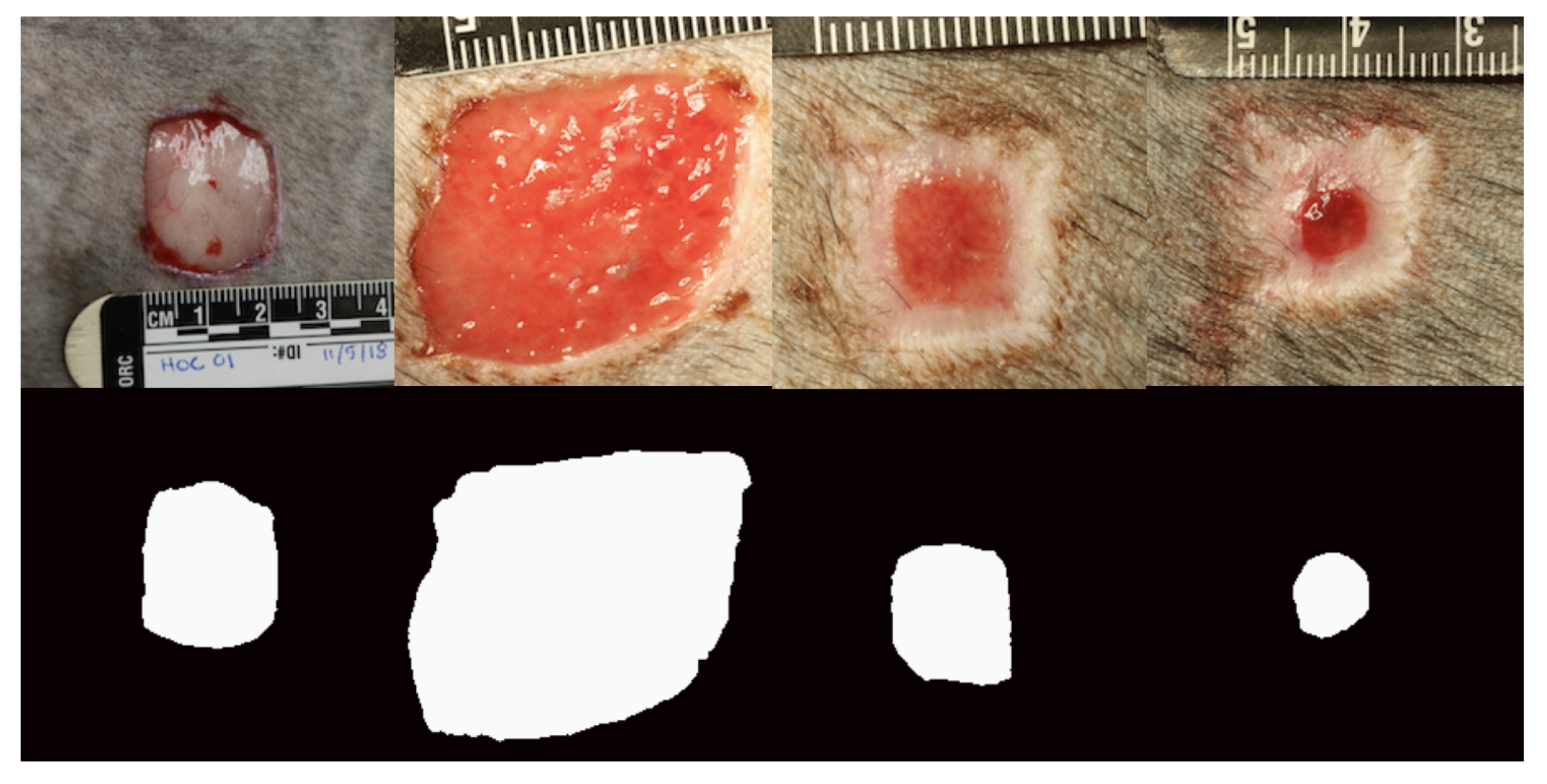
2.2.2. Dog Wound Healing Image Set

To train the regression model that predicts the time-to-healing from a digital wound image, we used a previously published [31] set of 136 color images (4000 × 6000 px; acquired every other day over 32 days and labeled by date) of ten 2 × 2 cm2 dog cutaneous surgical wounds (full-thickness surgical wounds in the trunk; see Ref. [31] for details). The ten dogs were male adult beagles (13–18 weeks of age). The wound images included standard rulers which enabled conversion of mm2 to px2 (Section 2.9). Given the size of the segmentation models (Section 2.6 and Section 2.7), to fit a reasonably sized batch of training images into the GPU memory, we resized and cropped the raw wound images to 224 × 224 px, to prepare them for feature extraction using the previously trained binary segmentation models. We augmented the 224 × 224 px wound-bed images as described in Section 2.3.1. To enable the use of the dog wound images for training the segmentation model, we manually segmented the images as described in Section 2.3.2 (Figure 2).

2.3. Image Augmentation and Annotation

2.3.1. Augmentor

To geometrically augment (e.g., rotate or flip) the sets of wound images used in this study, we used the Augmentor [11] tool as described in the Supplementary Materials Table S1, yielding four augmented images for each dog wound image. In this study, we compared the performances of different wound segmentation algorithms trained on original images (without augmentation) as well as algorithms trained on augmented image sets (see Section 3.2).

2.3.2. Pixel Annotation

To binary-segment wound images at the pixel level as “in-wound” our “not in wound” with human guidance, we used the PixelAnnotationTool software tool (ver. 0.14.0), which uses the marker-based variant of the watershed segmentation algorithm [37] from the OpenCV software library [38]. The manually annotated wound image masks were used as labeled data for training the segmentation algorithms (Section 2.11.2).

2.4. Superpixel Classifier Model Architecture

To classify the wound image superpixels by tissue type (not wound, fibrin, granulation, and necrotic), we implemented a six-layer perceptron [39] with rectified linear unit (ReLU) activation in each intermediate hidden layer and softmax activation with four classes in the output layer. For each of the four classes, we measured the model’s prediction performance by computing the area under the receiver-operating characteristic (AUROC) curve for the class’s prediction scores using the one vs. rest strategy [40] for comparison.

2.5. Segmentation

In our two-classe segmentation model architectures, SegNet (Section 2.6) and U-Net (Section 2.7), we do not use recurrent edges, whose use in segmentation has been advocated [41] in applications requiring multiscale object recognition (which is not an issue in our application). The two main classes of segmentation model architectures are described in the following two subsections.

2.6. SegNet Model Architecture

Of the two classes of neural network architectures that we used for image segmentation, the first is SegNet [35], a ten-layer convolutional network. SegNet is built on the FCN [23] architecture, which consists of an encoder network that computes a set of compact feature maps on high-resolution images, a decoder network that upsamples the feature maps, and a pixel-wise classification layer that outputs the full-size segmentation masks. The main difference separating a SegNet model from a common FCN model is that the decoder layers of a SegNet model directly use the pooling indices computed in the corresponding encoder layers’ max-pooling step. In this way, when a decoder layer performs the nonlinear upsampling of its lower-resolution input feature map from the previous layer, there is no need to learn the weights of the decoder part to upsample again. The advantages of reusing max-pooling indices include drastically reducing the number of parameters needed in the training process, improved on boundary delineation, and minimal modification required to implement upsampling. The encoder network is constructed by stacking basic computation blocks like convolution, nonlinear transformation using ReLU activation function, spatial pooling, and local response normalization [42]. To produce probability maps, a softmax layer is appended to the end of the network. To mitigate the downscaling effects of the convolution and pooling layers, the decoder network of the SegNet model is constructed by a stack of layers with upsampling operations. From the pixel-level probabilities, a threshold of 0.5 is used to produce the segmentation mask.

2.7. U-Net Model Architecture

The second class of the segmentation network architecture that we evaluated is U-Net [36], a U-shaped, 23-layer FCN. To localize, high-resolution features from the contracting path are combined with the upsampled output; a successive convolution layer can then learn to assemble a more precise output based on this more detailed information. U-Net has many feature channels in the upsampling part, which allow the network to propagate context information to higher resolution layers. U-Net does not have any fully connected layers and only uses the valid part of each convolution, allowing the segmentation of arbitrarily large images by an overlap-tile strategy (which also enables training on high-resolution images). For border region prediction, the missing context is extrapolated by mirroring the input image. At each downsampling step, the number of feature filters is doubled. The contracting path has repeated two 3 × 3 convolution layers (unpadded convolutions), each followed by a ReLU activation layer and a 2 × 2 max pooling operation with stride 2 for downsampling. The expanding path has an upsampling of the feature map followed by a 2 × 2 convolution layer (“up-convolution”) that halves the number of feature filters, a concatenation with the correspondingly cropped feature map from the contracting path, and two 3 × 3 convolutions, each followed by a ReLU activation layer. A 1 × 1 convolution is used to map each 64-component feature vector (each component is a feature filter) to the desired number of classes at the final layer. The U-Net has been reported to work well for segmentation applications with small training sets [28].

2.8. Feature Engineering and Extraction

We extracted features from both the Phase 2 (superpixel tissue-type classifier) model and from the Phase 1, Step 1 (pixel-level binary segmentation) models, as described below.

2.8.1. Feature Extraction from a Superpixel Model

For each of the four wound-tissue types (Section 2.2.1), we estimated the proportion of the wound image of that type adding up the prediction value for that type’s softmax class output across all superpixels. This procedure generated four features per image.

2.8.2. Feature Extraction from Segmentation Models

We extracted features from the segmentation models (Section 2.6 and Section 2.7) in two ways—using the network’s inner layer states as a vector encoding of the image, and by calculating summary statistics on the pixel-level binary segmentation (which were appended to the encoding vector).

Inner Layer Encoding

For the SegNet architecture (Section 2.6), we used the output of the intermediate layer “Conv5” as a feature vector. For the SegNet-1 network, the “Conv5” layer’s dimension is 6272, and thus, we reduced it using PCA (see Section 2.8.3) to 404 principal components. For the SegNet-2 network, the “Conv5” layer’s dimension is 1568 and we directly used that layer’s values as the feature vector. For the U-Net architecture in Section 2.7, we used the output of intermediate layer “Conv5” as a feature vector. For the U-Net-1 network, the “Conv5” layer’s dimension is 50,176, and thus, we reduced it using PCA to 342 principal components. From the U-Net-2 network, the “Conv5” layer’s dimension is 3136 and we used that layer’s values directly as the feature vector.

Wound Area Calculation

For each segmented wound image, from the pixel-level segmentation mask, we computed two summary-level features, the overall pixel wound area (see also Section 2.9), and the percentage of pixels of the image that are in the wound area. These two features were added to the “Conv5”-derived features to generate the complete Phase 1 feature-set for use in the regression.

2.8.3. PCA Reduction in Segmentation Feature Vectors

We carried out PCA using the function “PCA” from the sklearn.decomposition package, with parameter svd_solver set to “full” and parameter n_components set to 0.95 (which selects the number of principal components so that it explains at least 95% of the variance in the feature vector).

2.9. How We Obtained the Dependent Variable for Regression Training

Using the output from the segmentation models (Section 2.8.2), we first determined the length scale “ratio” of each image by calculating the pixel length of 1 cm space on the ruler in the image (manually counted by visual image inspection). We obtained the predicted wound area by counting the pixel area on the segmentation mask annotations and converted it to area in cm2 using the empirically determined linear pixel density per cm of each image. With the predicted wound area for each image, we obtained the remaining proportion of wound area as a feature for each image by dividing the predicted wound area of the current day with the predicted wound area of day zero. In the healing status prediction task, we did not use the number of days post-injury as a feature; this is because we used the image date to determine the dependent variable (i.e., the number of days to full healing) for the regression.

2.10. Regression Model Training

We evaluated three general-purpose regression algorithms (which are well described in the literature and highly versatile) that are well suited to our problem from the standpoints of sample-size of our labeled image-set, the high dimensionality of the feature-space, and the fact that the features are continuous: random forest regression, Gaussian process regression, and XGBoost.

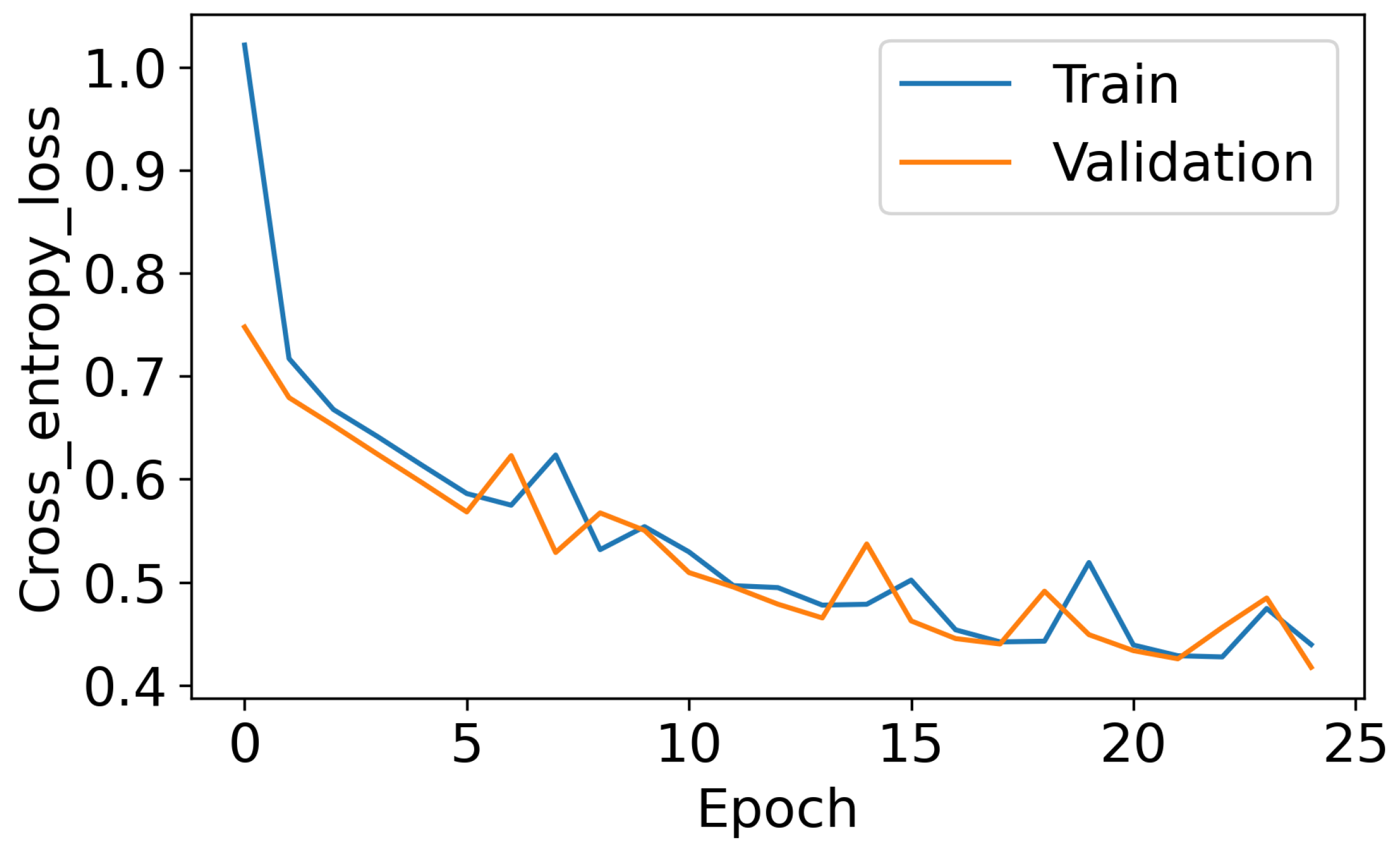
2.11. Model Training, Tuning, and Evaluation

We implemented cross-validation using RandomizedSearchCV and GridSearchCV from the package sklearn.model_selection, as described below. For all prediction evaluation metrics, we used functions from the sklearn.metrics package as described below.

2.11.1. Superpixel Classifier

For the Phase 2 classifier (Section 2.1.2 and Section 2.4), we used stratified ten-fold cross-validation (25 epochs) to obtain performance measurements (sample-averaged categorical cross-entropy loss) on the training-set images for hyperparameter tuning. We calculated the sample-averaged categorical cross-entropy loss as follows:
L = 1 N i , j y i j log y ^ i j ,
where j ranges over the four possible class labels, i ranges over the N samples, y i j is the ground-truth (one-hot encoded) class label for class label j for sample i, and y ^ i j is the prediction score for the class label j for sample i. We ultimately trained the model with a batch size of 1024 and for 25 epochs to using stochastic gradient descent [43] with a learning rate of 0.005, to minimize the categorical cross-entropy loss. For measuring AUROC on the test set of superpixels, we used the function “roc_auc_score” with the parameter “average” set to “weighted”.

2.11.2. Binary Pixel-Level Segmentation

For the image segmentation models (Section 2.6 and Section 2.7), we used five-fold cross-validation to obtain unbiased performance measures (precision, recall, and Dice overlap) on the training images for hyperparameter tuning. The hyperparameters were the number of epochs, batch size, and learning rate. We ultimately trained both SegNet models and both U-Net models with a batch size of two and for 2000 epochs (with early stopping) using stochastic gradient descent with a learning rate of 10−4 to minimize cross-entropy loss.

2.11.3. Regression Using Decision Trees or Gaussian Process

For Gaussian process regression, we used the class GaussianProcessRegressor from the package sklearn.gaussian_process; for random forest regression, we used the class RandomForestRegressor from the sklearn.ensemble package; and for XGBoost regression, we used the class XGBoostRegressor from the same package. For Random Forest and XGBoost, we first tuned model hyperparameters using RandomizedSearchCV using a larger set and range of hyperparameters (six for random forest, and four for XGBoost); for the Gaussian process model, we did not use the random-search hyperparameter tuning. Then, for all three models, we carried out exhaustive grid search hyperparameter tuning using the GridSearchCV function from sklearn.model_selection (four hyperparameters for Gaussian process, six for random forest, and four for XGBoost); for both, we used five-fold cross-validation (see Ref. [42] for details). For XGBoost regression model with the Phase 2 features only, to avoid overfitting, the hyperparameter grid-search space was reduced as follows: max_depth { 1 , 2 , 3 } , learning_rate { 0.0005 , 0.001 , 0.005 , 0.01 , 0.05 } , and n_estimators { 10 , 20 , 30 } .

2.11.4. Regression Using a Deep Neural Network

Using the Phase 1 (Section 2.1.1) and Phase 2 (Section 2.1.2) features as inputs and days until healing as the dependent variable (Section 2.9), we trained a five-layer fully connected deep neural network with ReLU activation functions and with the following numbers of neurons at each layer: 256, 128, 64, 32, and 1.

2.11.5. Confidence Interval Estimation

For the regression task, we estimated ±1 σ confidence intervals for the test-set coefficient of variation ( R 2 ) using bootstrap resampling [44] with 1000 iterations.

3. Results

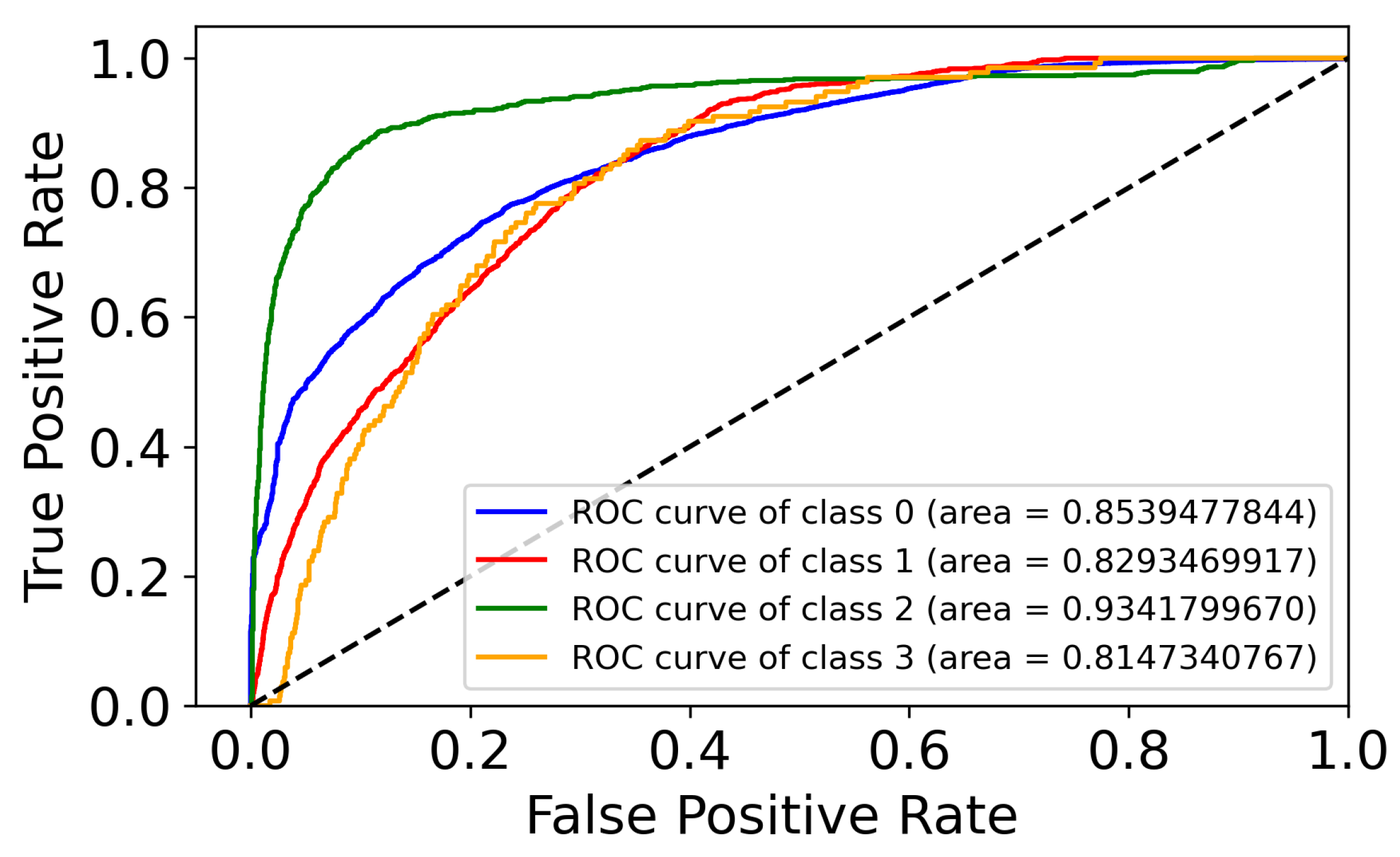
3.1. Superpixel Tissue-Type Classification Performance

Under the premise that for predicting time-to-healing, the utility of features extracted from a tissue-type multiclass superpixel classifier depends on the classifier’s performance, we investigated (Section 2.4) the MLP model’s performance for annotating non-overlapping 70 × 70 px wound image superpixels. For this analysis, we used the ULCER_SET (44,893 superpixels; see Section 2.2.1) in which each superpixel was expert-labeled with one of four tissue types [42].
We randomly separated the superpixels into training/validation and test sets (80% and 20%, respectively), tuned the classifier hyperparameters as described in Section 2.11.1, and obtained categorical cross-entropy loss on both the training/validate and test sets of superpixels and AUROC model performance (each class against all others) on the test set of superpixels. The prediction error on the test set was comparable to the training set (Figure 3), indicating that the model was not overfitted. The single-class-versus-others AUROC prediction performance exceeded 0.8 for all classes except class 3 (necrotic) (Figure 4); performance was best for discriminating class 2 (granulation) superpixels from the other superpixel classes (AUROC 0.94). The overall accuracy of the model for superpixel type prediction was 86.4% (which is comparable to the MLP results in Blanco et al. [9]).
Having measured the accuracy of the wound image superpixel classifier, we calculated, for each image, four summary features representing the total sum (across all superpixels of the image) of the class-specific prediction scores (Section 2.1.2); these four features are the “Phase 2” features, whose relative utility for the healing-time prediction regression task we evaluate in Section 3.4.

3.2. Binary Segmentation (Phase 1, Step 2) Model Performance to Find the Best Four Models

Under the premise that, for predicting wound time-to-healing, the utility of features derived from the pixel-level segmentation model will depend on the segmentation model’s performance, we investigated (Section 2.6 and Section 2.7) the performance of four neural network architectures (SegNet-1, SegNet-2, U-Net-1, and U-Net-2) for binary pixel-level segmentation. For this model-selection task, used a set of 136 high-resolution dog wound images [31] that had been pixel-wise labeled (Section 2.2.2) by human annotators as “within wound” or “outside wound”. Of the 136 dog wound images, we set aside 26 images (images from two wounds every 48 h) as a test-set of labeled images for evaluating the performance of the trained regression models (Section 3.3); we used the other 110 images for both segmentation model selection and for training the regression models. Given previous reports that image-set geometric augmentation improves the learning performance in some computer-vision tasks [45] and does not improve performance in others [46], we investigated the performance of the four network architectures using the original dog wound image set (“OIS”: 74 images) and using an augmented (Section 2.3.1) image set (“AIS”: 945 images).
We randomly partitioned the 110 images into 74 “OIS” images (images from five wounds) for training/validation and 36 images (images from three wounds) for model testing; we augmented 945 “AIS” images from 74 “OIS” images for training/validation and the same 36 original (unaugmented) images for testing. Using the training/validation set, we tuned the hyperparameters as described in Section 2.11.2. Then, for each of the eight combinations of the network architecture and image set (“AIS” or “OIS”), we trained on the 74 images of “OIS” and 945 images of “AIS” and measured the average performance on the test image-set by precision, recall, and Dice overlap. SegNet-1/AIS has the highest recall (0.953) and Dice coefficient (0.921) values (Table 1), whereas U-Net-1/AIS had the highest average precision (0.962).
For all architectures except U-Net-2, the performance was higher when trained on AIS than when trained on OIS; on average, augmentation improved performance by 7.7%. We selected the best model within each architecture type, to take forward to use for extracting segmentation-based features for time-to-healing prediction: SegNet-1/AIS, SegNet-2/OIS, U-Net-1/AIS, and U-Net-2/OIS. We then extracted image-level features from each of the four models using intermediate-layer neuron values (Section 2.8); due to the high dimensionality of these layers in SegNet-1 and U-Net-1, we reduced the dimensions for the SegNet-1 (Section 2.6) and U-Net-1 (Section 2.7) derived features using PCA. We combined the segmentation-derived features with the superpixel classification-derived features (Section 2.1.2)

3.3. Time-to-Healing Prediction Performance without Phase 2 Features

Next, we turned to the regression task of predicting, from features extracted from the wound image segmentation (i.e., not including the superpixel-based features), the number of days remaining for the wound to heal. We used the features extracted from one of the four binary segmentation models in Phase 1, Step 2 (with PCA used to reduce the dimension of the segmentation vectors extracted from SegNet-1 and U-Net-1, as described in Section 3.2), yielding a total of 404 features per image for SegNet-1 and 342 features per image for U-Net-1. We then added two summary-level features derived from the segmentation, consisting of the wound area and wound percentage area (see Section 2.8.2). Next, for the labeled training examples, we used a collection of 544 augmented time-series images of ten dog wounds (Section 2.2.2) from a controlled study of wound healing [31], for which we estimated (Section 2.8) the time-until-complete-healing (i.e., the dependent variable for the regression) for each of the images. We sought to evaluate three different regression algorithms, (Gaussian process regression, random forest regression, and XGBoost regression) separately against the feature-sets from the four different segmentation models for a set of 12 models. Using the set of 440 augmented (110 unaugmented images) dog images (images of eight different wounds), we tuned (Section 2.11.3) the regression algorithms’ hyperparameters and then trained each of the 12 models. Using either the 104 augmented (or 26 original) dog images (from two wounds) that were withheld as a test set, we obtained the average coefficient of variation ( R 2 ) performance measurements, for each of the 12 models. The combination of XGBoost with the SegNet-1/AIS-derived features had the best regression performance, with R 2 = 0.839 (Table 2) (SegNet-1/AIS also yielded the best segmentation performance; Table 1).
While the SegNet-1/AIS/XGBoost performance is only slightly better (0.839 vs. 0.831) than SegNet-1/AIS/Random-Forest, XGBoost trained faster than Random Forest (63 min vs. 118 min) than the RFR model when using the SegNet-1-PCA feature vector. Overall, across the four feature sets, XGBoost regression models had a 3.8% better performance than GPR models and 1.1% better than the random forest.

3.4. Time-to-Healing Prediction Performance including Phase 2 Features

Having established (Section 3.3) that the combination of using the SegNet-1 model (Section 2.6) for segmentation (trained with image augmentation) and using XGBoost for regression has the best performance among models tested for predicting wound time-to-healing, we next investigated whether adding four features derived (Section 2.8.1) from the superpixel tissue-type classifier (Section 2.4; i.e., Phase 2 of our method, as shown in Figure 1), which would improve the performance for the time-to-healing prediction. On the same train/validation and test sets of images as used for the regression model using only the segmentation (Phase 1) features (Section 3.3), we measured the average R 2 performance on the training/validation and test image sets, for two XGBoost regression models: a “Phase 1 model” trained with only the 406 SegNet-1 segmentation-derived features, and a “Phase 1 + 2 model” trained with all of those features plus four superpixel tissue type classifier-derived features (for a total of 410 features). We found that the test-set performance was higher for the “Phase 1 + 2 model” (0.863) than for the “Phase 1” model (0.839) (Table 3).
Finally, to compare the performance of the hybrid approach (consisting of deep learning-derived features and decision tree-based regression, as shown in Figure 1) with a fully neural network approach, we implemented an alternative fully neural-network-based approach in which the same Phase 1 and Phase 2 features were used as inputs to a deep neural network regression model (see Section 2.11.4 for details). The fully neural network approach’s R 2 performance (0.823 on CV, and 0.813 on the test set) was significantly lower than with the XGBoost-based hybrid approach (0.966 on CV, and 0.863 on the test set).

4. Discussion

Our the first point of discussion concerns the biological rationale for including image-wide tissue type (superpixel)-derived features in the regression model. The results of Section 3.1 indicate that the MLP model can accurately predict wound image superpixels’ tissue types among four classes (Section 2.2.1). Biologically, at the hemostasis (blood clotting) stage, platelets in the blood adhere to the injured site [47]. Platelet activation leads to the activation of fibrin, which autopolymerizes and further promotes platelet aggregation. Thus, a high proportion of “fibrin”-labeled tissue in the wound would be expected to indicate the healing process is in the early stage. Similarly, at the proliferative stage, granulation tissue can be noted from the healthy wound buds that protrude from the wound base [5]; thus, the proportion of “granulation”-labeled tissue would be expected to correlate with the healthy healing process, whereas the proportion of “necrosis”—(i.e., tissue death)-labeled tissue would be expected to be anti-correlated with time-to-healing. The size of superpixels represents a balance between the potential resolution for mapping tissue types in the wound-bed and accuracy for detecting tissue types based on color and texture patterns within the superpixel; in our case, in the dataset of labeled superpixels that we had access to, the superpixel size was chosen to be 70 × 70 px to balance those two priorities.
A second point of discussion concerns the (currently manual) step of counting pixels per cm in order to assess the wound area (which was necessary in order to estimate the days until healing, as explained in Section 2.9). Approaches toward automating this step could include (1) using the Hough transform [48] for detecting the ruler line; (2) using a separate neural network specifically for ruler detection and length calculation; or (3) using image metadata regarding image distance and field size to calculate the field’s physical dimensions.
While the results of Table 3 represent a significant new finding in terms of the types of features that are useful for predicting the wound time-to-healing, the context of the dataset is relevant to interpreting the model’s absolute performance. The ground-truth set of labeled images used for the regression model in this work are from a series of controlled images (acquired with a single digital camera at fixed distance) from a controlled study [31] of surgical wounds. Thus, we would expect that attaining equivalent absolute predictive performance on wound images from uncontrolled data acquisition settings and from a broader array of wound conditions (e.g., burns, ulcers, etc.) would likely require retraining the regression model with a substantially larger and more diverse set of images. However, the key findings from this work (Table 1, Table 2 and Table 3) are based on the relative regression performance on a feature set including superpixel tissue-derived features vs. without them. Although the superpixel tissue-derived features (Phase 2 features) by themselves have relatively poor performance on the regression task (see Table 3), when combined with the segmentation-derived features (Phase 1 features) they significantly improve the regression performance.
As far as we are aware, this work represents the first effort to leverage wound images from a controlled study of surgical wound healing for the purpose of regression model selection and feature-set selection for computationally predicting wound time-to-healing. Our long-term goal is to apply these results to develop models for predicting healing time in humans. Furthermore, a natural progression of the work would be to integrate wound images with other measurements such as C-reactive protein (CRP) [49] and immunoglobulin G [50], as well as relevant clinical comorbidities and demographic/anthropometric parameters (e.g., diabetes, nutritional status, age, body mass index, and smoking status) [13] to accurately predict the time-to-healing in human clinical settings and to flag wounds requiring intervention. While these types of demographic, anthropometric, and comorbidity data were not needed for the specific questions that we focused on in this controlled study of canine wound healing (i.e., Can a tissue type-augmented hybrid approach improve time-to-healing prediction? and Which regression model leveraging a hybrid tissue-type and segmentation-derived feature-set gives best performance for time-to-healing prediction?), it is expected that such data would be required in order to maximize accuracy in clinical settings.

5. Conclusions

For three of the four image segmentation models, using the augmented wound image set led to a better image segmentation performance than the models learned using original images without augmentation. Among the four segmentation models, the SegNet-1-PCA model using augmented images had the highest test-set Dice performance (0.921). Using the segmentation-derived features, out of the three different regression models that we studied, XGBoost regression outperformed both Gaussian process regression and random forest regression, reaching a test-set R 2 of 0.839 (95% confidence range of 0.825–0.852). We further found that, given the high-resolution wound images without tissue type labels, the SegNet-PCA model is a powerful tool for extracting low-dimensional feature vectors while generating reasonable wound segmentation masks; this yields a mask that retains the wound area information and features that retain biological patterns that enable the improved image-based prediction of wound time-to-healing. Finally, we demonstrated that incorporating tissue-type superpixel-derived features into the regression model significantly improves the prediction of wound time-to-healing, versus using features derived only from the image segmentation model.

Supplementary Materials

The following supporting information can be downloaded at: https://www.mdpi.com/article/10.3390/computation12030042/s1, Table S1: Dog wound image augmentation transformations used.

Author Contributions

Overall study design: S.A.R., Q.W. and A.K.; implementation of computational approach: Q.W. and A.K.; Data analysis: A.K., Q.W. and S.A.R.; manuscript writing: S.A.R., A.K. and Q.W. All authors have read and agreed to the published version of the manuscript.

Funding

This work was supported by the National Institutes of Health [grant number R01EB028104].

Institutional Review Board Statement

Not applicable.

Informed Consent Statement

Not applicable.

Data Availability Statement

The Python and Tensorflow source code for our wound image analysis method is available on GitHub at https://github.com/ramseylab/wound-analysis (accessed on 26 February 2024). under an open source software license. The ULCER_SET images from the Blanco et al. study [9] are freely and publicly available on GitHub at https://github.com/gu-blanco/qtdu (accessed on 26 February 2024). The dog wound images that were used in the study were previously published by Kurach et al. [31] and were provided to us courtesy of one of that study’s co-authors (Bryden Stanley at Michigan State University); the images are available from Stanley upon request.

Acknowledgments

We thank Elain Fu, Matt Johnston, and Arun Natarajan for their ideas and feedback on the project. We thank Bryden J. Stanley and Milan Milovancev for kindly providing the wound images from Ref. [31].

Conflicts of Interest

The authors declare no conflicts of interest. The funders had no role in the design of the study; in the collection, analyses, or interpretation of data; in the writing of the manuscript; or in the decision to publish the results.

Abbreviations

The following abbreviations are used in this manuscript:
AISaugmented image set
AUROCarea under the receiver operating characteristic curve
CVcross-validation
FCNfully convolutional network
MLPmulti-layer perceptron
OISoriginal image set
PCAprincipal components analysis
pxpixel
R 2 coefficient of determination
ReLUrectified linear unit

References

  1. Branski, L.K.; Gauglitz, G.G.; Herndon, D.N.; Jeschke, M.G. A review of gene and stem cell therapy in cutaneous wound healing. Burns 2009, 35, 171–180. [Google Scholar] [CrossRef]
  2. McLister, A.; McHugh, J.; Cundell, J.; Davis, J. New Developments in Smart Bandage Technologies for Wound Diagnostics. Adv. Mater. 2016, 28, 5732–5737. [Google Scholar] [CrossRef]
  3. Sen, C.K.; Gordillo, G.M.; Roy, S.; Kirsner, R.; Lambert, L.; Hunt, T.K.; Gottrup, F.; Gurtner, G.C.; Longaker, M.T. Human skin wounds: A major and snowballing threat to public health and the economy. Wound Repair Regen. 2009, 17, 763–771. [Google Scholar] [CrossRef]
  4. Falcone, M.; Angelis, B.D.; Pea, F.; Scalise, A.; Stefani, S.; Tasinato, R.; Zanetti, O.; Paola, L.D. Challenges in the management of chronic wound infections. J. Glob. Antimicrob. Resist. 2021, 26, 140–147. [Google Scholar] [CrossRef]
  5. Grey, J.E.; Enoch, S.; Harding, K.G. Wound assessment. BMJ 2006, 332, 285–288. [Google Scholar] [CrossRef]
  6. Seaman, M.; Lammers, R. Inability of patients to self-diagnose wound infections. J. Emerg. Med. 1991, 9, 215–219. [Google Scholar] [CrossRef]
  7. Wang, C.; Yan, X.; Smith, M.; Kochhar, K.; Rubin, M.; Warren, S.M.; Wrobel, J.; Lee, H. A unified framework for automatic wound segmentation and analysis with deep convolutional neural networks. In Proceedings of the 37th Annual International Conference of the IEEE Engineering in Medicine and Biology Society, Milan, Italy, 25–29 August 2015; pp. 2415–2418. [Google Scholar] [CrossRef]
  8. Veredas, F.J.; Luque-Baena, R.M.; Martín-Santos, F.J.; Morilla-Herrera, J.C.; Morente, L. Wound image evaluation with machine learning. Neurocomputing 2015, 164, 112–122. [Google Scholar] [CrossRef]
  9. Blanco, G.; Traina, A.J.M.; Traina, C., Jr.; Azevedo-Marques, P.M.; Jorge, A.E.S.; de Oliveira, D.; Bedo, M.V. A superpixel-driven deep learning approach for the analysis of dermatological wounds. Comput. Methods Programs Biomed. 2020, 183, 105079. [Google Scholar] [CrossRef] [PubMed]
  10. Anisuzzaman, D.M.; Patel, Y.; Rostami, B.; Niezgoda, J.; Gopalakrishnan, S.; Yu, Z. Multi-modal wound classification using wound image and location by deep neural network. Sci. Rep. 2022, 12, 20057. [Google Scholar] [CrossRef]
  11. Bloice, M.D.; Roth, P.M.; Holzinger, A. Biomedical image augmentation using Augmentor. Bioinformatics 2019, 35, 4522–4524. [Google Scholar] [CrossRef] [PubMed]
  12. Zhang, R.; Tian, D.; Xu, D.; Qian, W.; Yao, Y. A Survey of Wound Image Analysis Using Deep Learning: Classification, Detection, and Segmentation. IEEE Access 2022, 10, 79502–79515. [Google Scholar] [CrossRef]
  13. Berezo, M.; Budman, J.; Deutscher, D.; Hess, C.T.; Smith, K.; Hayes, D. Predicting Chronic Wound Healing Time Using Machine Learning. Adv. Wound Care 2022, 11, 281–296. [Google Scholar] [CrossRef]
  14. Sullivan, T.P.; Eaglstein, W.H.; Davis, S.C.; Mertz, P. The pig as a model for wound healing. Wound Repair Regen. 2001, 9, 66–76. [Google Scholar] [CrossRef] [PubMed]
  15. Volk, S.W.; Bohling, M.W. Comparative wound healing—Are the small animal veterinarian’s clinical patients an improved translational model for human wound healing research? Wound Repair Regen. 2013, 21, 372–381. [Google Scholar] [CrossRef] [PubMed]
  16. Stockman, G.; Shapiro, L.G. Computer Vision, 1st ed.; Prentice Hall: Hoboken, NJ, USA, 2001. [Google Scholar]
  17. Gupta, S.; Arbelaez, P.; Malik, J. Perceptual Organization and Recognition of Indoor Scenes from RGB-D Images. In Proceedings of the IEEE Conference on Computer Vision and Pattern Recognition, Portland, OR, USA, 23–28 June 2013; pp. 564–571. [Google Scholar] [CrossRef]
  18. Silberman, N.; Hoiem, D.; Kohli, P.; Fergus, R. Indoor Segmentation and Support Inference from RGBD Images. In Proceedings of the Computer Vision–ECCV 2012, Florence, Italy, 7–13 October2012; Fitzgibbon, A., Lazebnik, S., Perona, P., Sato, Y., Schmid, C., Eds.; Springer: Berlin/Heidelberg, Germany, 2012; pp. 746–760. [Google Scholar]
  19. Song, B.; Sacan, A. Automated wound identification system based on image segmentation and Artificial Neural Networks. In Proceedings of the International Conference on Bioinformatics and Biomedicine, Philadelphia, PA, USA, 4–7 October 2012; pp. 1–4. [Google Scholar] [CrossRef]
  20. Hettiarachchi, N.; Mahindaratne, R.; Mendis, G.; Nanayakkara, H.; Nanayakkara, N.D. Mobile based wound measurement. In Proceedings of the Point-of-Care Healthcare Technologies, Bangalore, India, 16–18 January 2013; pp. 298–301. [Google Scholar]
  21. Fauzi, M.F.A.; Khansa, I.; Catignani, K.; Gordillo, G.; Sen, C.K.; Gurcan, M.N. Computerized segmentation and measurement of chronic wound images. Comput. Biol. Med. 2015, 60, 74–85. [Google Scholar] [CrossRef] [PubMed]
  22. Cui, C.; Thurnhofer-Hemsi, K.; Soroushmehr, R.; Mishra, A.; Gryak, J.; Dominguez, E.; Najarian, K.; Lopez-Rubio, E. Diabetic Wound Segmentation using Convolutional Neural Networks. In Proceedings of the 41st Annual International Conference of the IEEE Engineering in Medicine and Biology Society, Berlin, Germany, 23–27 July 2019; pp. 1002–1005. [Google Scholar] [CrossRef]
  23. Long, J.; Shelhamer, E.; Darrell, T. Fully convolutional networks for semantic segmentation. In Proceedings of the Conference on Computer Vision and Pattern Recognition, Boston, MA, USA, 7–12 June 2015; pp. 3431–3440. [Google Scholar]
  24. Yuan, Y.; Chao, M.; Lo, Y.C. Automatic Skin Lesion Segmentation Using Deep Fully Convolutional Networks With Jaccard Distance. IEEE Trans. Med. Imaging 2017, 36, 1876–1886. [Google Scholar] [CrossRef] [PubMed]
  25. Milletari, F.; Navab, N.; Ahmadi, S.A. V-net: Fully convolutional neural networks for volumetric medical image segmentation. In Proceedings of the 4th International Conference on 3D Vision, Stanford, CA, USA, 25–28 October 2016; pp. 565–571. [Google Scholar]
  26. Goyal, M.; Yap, M.H.; Reeves, N.D.; Rajbhandari, S.; Spragg, J. Fully convolutional networks for diabetic foot ulcer segmentation. In Proceedings of the International Conference on Systems, Man, and Cybernetics, Banff, AB, Canada, 5–8 October 2017; pp. 618–623. [Google Scholar] [CrossRef]
  27. Liu, X.; Wang, C.; Li, F.; Zhao, X.; Zhu, E.; Peng, Y. A framework of wound segmentation based on deep convolutional networks. In Proceedings of the 10th International Congress on Image and Signal Processing, Biomedical Engineering and Informatics, Shanghai, China, 14–16 October 2017; pp. 1–7. [Google Scholar]
  28. Wang, C.; Anisuzzaman, D.M.; Williamson, V.; Dhar, M.K.; Rostami, B.; Niezgoda, J.; Gopalakrishnan, S.; Yu, Z. Fully automatic wound segmentation with deep convolutional neural networks. Sci. Rep. 2020, 10, 21897. [Google Scholar] [CrossRef] [PubMed]
  29. Sandler, M.; Howard, A.; Zhu, M.; Zhmoginov, A.; Chen, L.C. Mobilenetv2: Inverted residuals and linear bottlenecks. In Proceedings of the Conference on Computer Vision and Pattern Recognition, Salt Lake City, UT, USA, 18 –23 June 2018; pp. 4510–4520. [Google Scholar]
  30. Achanta, R.; Shaji, A.; Smith, K.; Lucchi, A.; Fua, P.; Süsstrunk, S. SLIC Superpixels Compared to State-of-the-Art Superpixel Methods. IEEE Trans. Pattern Anal. Mach. Intell. 2012, 34, 2274–2282. [Google Scholar] [CrossRef] [PubMed]
  31. Kurach, L.M.; Stanley, B.J.; Gazzola, K.M.; Fritz, M.C.; Steficek, B.A.; Hauptman, J.G.; Seymour, K.J. The Effect of Low-Level Laser Therapy on the Healing of Open Wounds in Dogs. Vet. Surg. 2015, 44, 988–996. [Google Scholar] [CrossRef] [PubMed]
  32. Rasmussen, C.E.; Williams, C.K.I. Gaussian Processes for Machine Learning; MIT Press: Cambridge, MA, USA, 2005. [Google Scholar] [CrossRef]
  33. Breiman, L. Random Forests. Mach. Learn. 2001, 45, 5–32. [Google Scholar] [CrossRef]
  34. Chen, T.; Guestrin, C. XGBoost. In Proceedings of the 22nd ACM SIGKDD International Conference on Knowledge Discovery and Data Mining, San Francisco, CA, USA, 13–17 August 2016; pp. 785–794. [Google Scholar] [CrossRef]
  35. Badrinarayanan, V.; Kendall, A.; Cipolla, R. SegNet: A deep convolutional encoder-decoder architecture for image segmentation. IEEE Trans. Pattern Anal. Mach. Intell. 2017, 39, 2481–2495. [Google Scholar] [CrossRef] [PubMed]
  36. Ronneberger, O.; Fischer, P.; Brox, T. U-Net: Convolutional Networks for Biomedical Image Segmentation. In Proceedings of the Medical Image Computing and Computer-Assisted Intervention, Munich, Germany, 5–9 October 2015; Navab, N., Hornegger, J., Wells, W.M., Frangi, A.F., Eds.; Springer: Berlin/Heidelberg, Germany, 2015; pp. 234–241. [Google Scholar]
  37. Beucher, S. The Watershed Transformation Applied To Image Segmentation. Scanning Microsc. 1992, 6, 299–314. [Google Scholar]
  38. Bradski, G.; Kaehler, A. OpenCV. Dr. Dobb’s J. 2000, 3, 122–125. [Google Scholar]
  39. McCulloch, W.S.; Pitts, W. A logical calculus of the ideas immanent in nervous activity. Bull. Math. Biophys. 1943, 5, 115–133. [Google Scholar] [CrossRef]
  40. Stiller, C.; Lappe, D. Gain/cost controlled displacement-estimation for image sequence coding. In Proceedings of the International Conference on Acoustics, Speech, and Signal Processing, Toronto, ON, Canada, 14–17 May 1991; pp. 2729–2730. [Google Scholar] [CrossRef]
  41. Jiang, D.; Qu, H.; Zhao, J.; Zhao, J.; Liang, W. Multi-level graph convolutional recurrent neural network for semantic image segmentation. Telecommun. Syst. 2021, 77, 563–576. [Google Scholar] [CrossRef]
  42. Wei, Q. Machine Learning for Precision Medicine: Application to Cancer Chemotherapy Response Prediction and Wound Healing Status Assessment. Ph.D. Thesis, Oregon State University, Corvallis, OR, USA, 2021. [Google Scholar]
  43. Ruder, S. An overview of gradient descent optimization algorithms. arXiv 2016, arXiv:1609.04747. [Google Scholar]
  44. Hastie, T.; Tibshirani, R.; Friedman, J. The Elements of Statistical Learning; Springer Series in Statistics; Springer: New York, NY, USA, 2001. [Google Scholar]
  45. Anwar, T.; Zakir, S. Effect of Image Augmentation on ECG Image Classification Using Deep Learning. In Proceedings of the International Conference on Artificial Intelligence, Islamabad, Pakistan, 5–7 April 2021; pp. 182–186. [Google Scholar] [CrossRef]
  46. Elgendi, M.; Nasir, M.U.; Tang, Q.; Smith, D.; Grenier, J.P.; Batte, C.; Spieler, B.; Leslie, W.D.; Menon, C.; Fletcher, R.R.; et al. The Effectiveness of Image Augmentation in Deep Learning Networks for Detecting COVID-19: A Geometric Transformation Perspective. Front. Med. 2021, 8, 629134. [Google Scholar] [CrossRef]
  47. Kehrel, B.E. Blood platelets: Biochemistry and physiology. Hamostaseologie 2003, 23, 149–158. [Google Scholar]
  48. Duda, R.O.; Hart, P.E. Use of the Hough Transformation to Detect Lines and Curves in Pictures. Commun. Assoc. Comput. Mach. 1972, 15, 11–15. [Google Scholar] [CrossRef]
  49. Pepys, M.B.; Hirschfield, G.M. C-reactive protein: A critical update. J. Clin. Investig. 2003, 111, 1805–1812. [Google Scholar] [CrossRef]
  50. Vidarsson, G.; Dekkers, G.; Rispens, T. IgG Subclasses and Allotypes: From Structure to Effector Functions. Front. Immunol. 2014, 5, 520. [Google Scholar] [CrossRef] [PubMed]
Figure 1. Overview of the two-phase approach that we developed for computationally predicting the time-to-healing from a wound image. (In the Phase 1 section, the inset wound images are the courtesy of Dr. Bryden J. Stanley (see Acknowledgements). In the Phase 2 section, the inset wound images are reprinted from the Blanco et al. study [9], © 2020 with permission from Elsevier (Amsterdam, The Netherlands)).
Computation 12 00042 g001
Figure 2. Example wound images (top row) and corresponding human-segmented images (bottom row) from the dog wound image dataset [31] used for training the healing-time model. Top-row images are cropped from original images that were provided courtesy of Dr. B. Stanley (see acknowledgments).
Computation 12 00042 g002
Figure 3. Average categorical cross-entropy loss of the MLP model for each of 25 training epochs, evaluated on the train/validate superpixels and on the test-set superpixels.
Computation 12 00042 g003
Figure 4. Test-set performance for classifying superpixels as class 0 (not-wound), class 1 (fibrin), class 2 (granulation), or class 3 (necrotic). Each receiver operating characteristic (ROC) curve represents the test-set performance on the binary task of predicting whether a superpixel is of the indicated class or not. The class sample counts as follows: Class 0, 7437 samples; Class 1, 794 samples; Class 2, 656 samples; and Class 3, 89 samples. “Area” denotes AUROC. Each ROC curve shows a relationship between sensitivity (the vertical axis) and the false positive error rate (the horizontal axis), for correctly recognizing superpixels that are members of one class versus mis-predictions of the other three class types. Each ROC curve rises steeply as easy cases are discriminated and then saturates as more borderline cases require increasingly permissive thresholds for making a positive prediction.
Computation 12 00042 g004
Table 1. Test-set performance (averaged over 36 images) of each of eight combinations of network architecture and training-set performance (original, i.e., OIS; or augmented, i.e., AIS) on the segmentation task of classifying the wound image pixels as “within wound” or “not within wound”. OIS: original image set (without augmentation); AIS: augmented image set.
ArchitectureSetPrecisionRecallDice
SegNet-1AIS0.9550.9530.921
SegNet-1OIS0.9620.7100.773
SegNet-2AIS0.9330.9060.887
SegNet-2OIS0.7400.9200.787
U-Net-1AIS0.9620.9500.916
U-Net-1OIS0.9460.8830.878
U-Net-2AIS0.9300.9370.890
U-Net-2OIS0.9520.9480.919
Table 2. Average prediction performance of three regression models—each with input features from one of four different segmentation models—on a test set of 104 images (26 original images of two dog wounds; four-fold augmented as described in Section 2.3.1), as measured by R 2 coefficient of variation. The models shown here were trained with Phase 1 features only; they did not include any superpixel-derived (i.e., Phase 2) features. Column abbreviations as follows: Arch., segmentation network architecture; PCA, indicates whether or not that segmentation model’s image encoding was PCA-reduced; CV R 2 , cross-validation average R 2 on the set of 440 images used for training the regression model; Test R 2 , average R 2 on the test set of images; L.C.I., lower confidence interval (1 σ ) on the test R 2 ; U.C.I., upper confidence interval (1 σ ) on test R 2 .
ModelArch.PCA?Feat.CV R 2 Test R 2 L.C.I.U.C.I.
GPRU-Net-1Yes3440.9160.7730.7510.799
GPRU-Net-2No31380.7910.7620.7390.781
GPRSegNet-1Yes4060.9040.7780.7490.797
XGBoostU-Net-1Yes3440.9190.7660.7490.775
XGBoostU-Net-2No31380.8670.7950.7740.821
XGBoostSegNet-1Yes4060.9220.8390.8250.852
XGBoostSegNet-2no15700.8900.8110.7990.826
RFRU-Net-1yes3440.9140.7700.7650.785
RFRU-Net-2no31380.8480.7820.7690.803
RFRSegNet-1yes4060.9160.8310.8170.851
RFRSegNet-2no15700.8930.7970.7810.818
Table 3. Average prediction performance of XGBoost regression on a test set of 104 images (images from two different dog wounds; 4 × augmented from 26 original wound images), as measured by R 2 coefficient of variation, for models trained with 406 features (from SegNet-1 segmentation only) and/or with the four superpixel-derived tissue classification features (Section 2.8.1). Column abbreviations are as follows: Arch., segmentation network architecture; Phase, indicates which feature-sets were included; CV R 2 , cross-validation average R 2 on the augmented set of 440 images used for regression training; Test R 2 , average R 2 on the test set of images; L.C.I., lower-confidence interval (1 σ ) on test R 2 ; U.C.I., upper-confidence interval (1 σ ) on test R 2 . Performance on the Phase 2 only feature-set was sufficiently low that no C.I. permutation analysis was performed.
ModelArch.PhaseFeat.CV R 2 Test R 2 L.C.I.U.C.I.
XGBoostSegNet-11 and 24100.9660.8630.8510.875
XGBoostSegNet-114060.9220.8390.8250.852
XGBoostSegNet-1240.6030.042
Disclaimer/Publisher’s Note: The statements, opinions and data contained in all publications are solely those of the individual author(s) and contributor(s) and not of MDPI and/or the editor(s). MDPI and/or the editor(s) disclaim responsibility for any injury to people or property resulting from any ideas, methods, instructions or products referred to in the content.

