Article

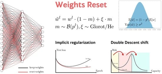
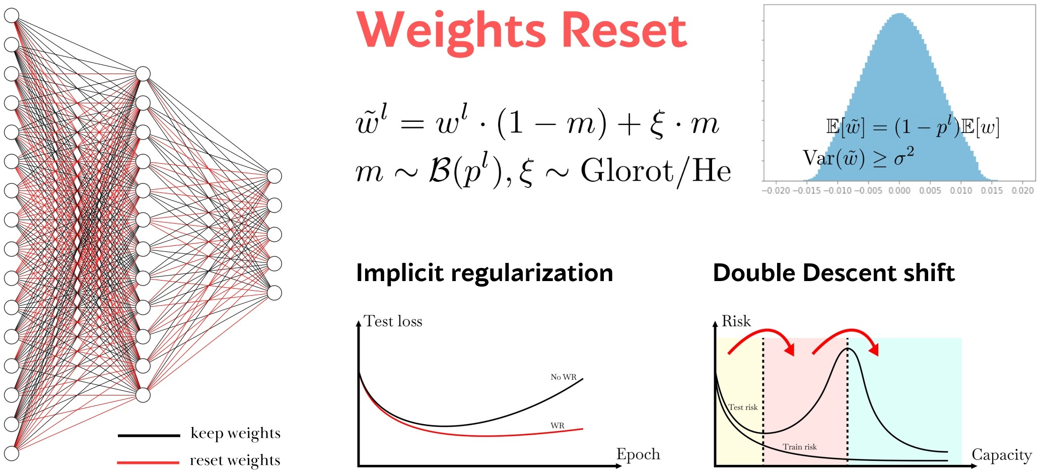
The Weights Reset Technique for Deep Neural Networks Implicit Regularization

by
Grigoriy Plusch
,
Sergey Arsenyev-Obraztsov
and
Olga Kochueva
*
Department of Applied Mathematics and Computer Modeling, National University of Oil and Gas “Gubkin University”, 65, Leninsky Prospekt, 119991 Moscow, Russia
*
Author to whom correspondence should be addressed.
Computation 2023, 11(8), 148; https://doi.org/10.3390/computation11080148
Submission received: 8 May 2023 / Revised: 26 July 2023 / Accepted: 27 July 2023 / Published: 1 August 2023

Abstract

:
We present a new regularization method called Weights Reset, which includes periodically resetting a random portion of layer weights during the training process using predefined probability distributions. This technique was applied and tested on several popular classification datasets, Caltech-101, CIFAR-100 and Imagenette. We compare these results with other traditional regularization methods. The subsequent test results demonstrate that the Weights Reset method is competitive, achieving the best performance on Imagenette dataset and the challenging and unbalanced Caltech-101 dataset. This method also has sufficient potential to prevent vanishing and exploding gradients. However, this analysis is of a brief nature. Further comprehensive studies are needed in order to gain a deep understanding of the computing potential and limitations of the Weights Reset method. The observed results show that the Weights Reset method can be estimated as an effective extension of the traditional regularization methods and can help to improve model performance and generalization.

Graphical Abstract

1. Introduction

Deep learning models have achieved remarkable success in various applications, including image classification, speech recognition, natural language processing, etc. However, these models are prone to overfitting. This situation occurs when a model learns to fit the training data too well, resulting in poor performance on new, unseen data. Regularization techniques are applied to prevent overfitting by adding constraints, even implicit, to the model parameters during training. The development of regularization methods has a long history, the main milestones of which are:
  • L1/L2 regularization. Originally, the idea of regularization was proposed by Tikhonov (it is known as Tikhonov regularization [1]), and was developed for the solution of ill-posed problems. It is effective as a method of estimating the coefficients of multiple-regression models in scenarios where the input variables are highly correlated which commonly occurs in models with large numbers of parameters (Ridge regression). Later the idea of regularization, particularly L1/L2 regularization, was applied to the solution of machine learning problems.
  • The concept of weight decay, which involves adding a penalty term to the error function to discourage large weights. It was first proposed in the context of neural networks in [2]. While this is not an implicit regularization method, it serves as a useful benchmark for later methods.
  • The trade-off between model complexity and generalization performance, which is an important theme in regularization. In [3], Lecun et al. proposed a technique called “optimal brain damage” that involves pruning the weights in a neural network to improve its generalization performance. It can be considered as a form of regularization since it reduces the number of parameters in the model and can help prevent overfitting.
  • Early stopping. Prechelt in [4] provided an analysis of the effectiveness of early stopping for neural network training, including an exploration of the optimal stopping point based on a validation set. Caruana in [5] explored the effects of early stopping on different optimization algorithms for neural networks, and provided a detailed analysis of the trade-off between overfitting and underfitting.
  • Dropout is a regularization technique proposed by Srivastava et al. in [6]. It involves randomly dropping out some of the neurons in a layer during training, which has the effect of preventing the network from overreliance on any one feature. Dropout is an implicit regularization technique because it introduces noise into the training process, which has a regularizing effect.
  • Batch normalization is a technique proposed by Ioffe and Szegedy in [7] that normalizes the inputs to each layer to have zero mean and unit variance. This has the effect of stabilizing the distribution of activations and gradients, which makes training more robust to hyperparameter choices and reduces the need for explicit regularization.
  • Data augmentation is a technique that involves generating new training examples by applying random transformations to the existing examples. This has the effect of increasing the size of the training set and making the model more robust to variations in the input. One of the earliest papers to introduce data augmentation in the context of image classification using neural networks was [8].
  • Implicit bias of optimization algorithms. The concept of implicit bias of optimization algorithms was introduced in [9]. This paper showed that the choice of an optimization algorithm can have a significant impact on the generalization performance of a neural network, even when the data are linearly separable. Specifically, the authors showed that gradient descent with weight decay implicitly imposes a bias towards solutions that have smaller L2 norm, which can explain the generalization performance of neural networks trained with this algorithm. The paper also introduced a framework for analyzing the implicit bias of optimization algorithms on different classes of data.
It is worth mentioning some recently published papers addressing the regularization problem. In [10], the authors argue that while the norm-based explanations of implicit regularization have been successful in many cases, they may not provide a complete picture of the phenomenon. Specifically, they propose that there may be other factors that contribute to the implicit regularization effects in deep learning, which cannot be captured by the norms of the weight matrices. To support this argument, the authors provide several examples of deep learning models that exhibit implicit regularization effects that cannot be fully explained by the norms of the weight matrices. For instance, they show that certain architectures, such as residual networks and attention-based models, can exhibit implicit regularization effects even when the norms of their weight matrices are relatively large. The authors also propose several hypotheses for the underlying mechanisms that contribute to the implicit regularization effects in deep learning, such as the geometry of the optimization landscape and the properties of the data distributions. They suggest that a more nuanced understanding of these mechanisms can lead to more effective and efficient deep learning algorithms.
In [11], the authors argue that many previous works have focused on characterizing implicit regularization using functions that are independent of the training data, such as the norm of the weight matrix or the singular values of the data matrix. While these functions can provide useful insights into the behavior of deep neural networks, they are limited in their ability to capture the full complexity of the optimization landscape. To illustrate this limitation, the authors present several examples of deep neural networks where the implicit regularization cannot be fully explained by data-independent functions. They show that in these cases, the optimization landscape has a non-trivial structure that depends on the specific properties of the training data, and that cannot be captured by simple functions.
In [12], the authors study a new optimization framework called Sharpness-Aware Minimization (SAM) that aims to improve the generalization performance of deep learning models. SAM is based on the idea that the optimization landscape of deep learning models can have flat regions that lead to poor generalization, and sharp regions that lead to good generalization. SAM aims to find a balance between the two by minimizing a combination of the training loss and a measure of the sharpness of the optimization landscape. The authors consider SAM through an implicit regularization lens and present a new theoretical explanation of the generalization performance of SAM.
In [13], the authors empirically identify three phases of learning that explain the impact of implicit regularization on the learning dynamics. They subsequently found that bootstrapping alone is insufficient to explain the collapse of the effective rank. They show that several other factors could confound the relationship between effective rank and performance and conclude that studying this association under simplistic assumptions could be highly misleading.
A large number of publications touching on various aspects of implicit regularization show that this issue is far from being exhausted and requires new research to build effective machine learning algorithms.
We propose a new regularization technique called Weights Reset that periodically resets a randomly selected part of the weights of a deep neural network in the process of training. The idea behind Weights Reset is to prevent the model from becoming stuck in unsatisfactory local minima by exploring other parts of the optimization landscape.
According to our knowledge, Weights Reset has not been proposed or studied in the literature before. We evaluate the effectiveness of Weights Reset by comparing it with other traditional forms of deep learning regularization techniques on several image classification datasets: CIFAR-100 [14], Caltech-101 [15], and Imagenette [16].
Computer vision (CV) tasks, alongside natural language processing, have long been recognized as some of the most complex problems in machine learning. In this study, we focus on the image classification problem, which is a widely studied and well-known task among researchers. By investigating the effects of our proposed Weights Reset technique on image classification, we aim to provide valuable insights and practical implications for the research community. The results obtained from our experiments not only contribute to the existing knowledge in CV but also serve as a starting point for future exploration of the Weights Reset technique in other machine learning tasks.
Our experiments show that Weights Reset can improve the generalization performance of deep neural networks, especially when the models are prone to overfitting.
The current research state of Weights Reset is still in its early stages, with limited empirical evidence of its effectiveness and comparison to other regularization techniques. Therefore, it is essential to evaluate the performance of Weights Reset against alternative approaches to determine its strength in preventing overfitting.
In addition, we can express a hypothesis that the Weights Reset technique may be associated with the phenomenon of Double Descent [17] in deep neural networks. However, there is a lack of research that directly supports this assumption. Double Descent refers to the counterintuitive observation that, under certain conditions, increasing the number of model parameters can initially lead to worse generalization errors before ultimately improving it. Despite its recent discovery, Double Descent has already become a subject of active research in the machine learning community. It is possible that Weights Reset may offer a new fresh perspective on this phenomenon.
Overall, our investigation contributes to the ongoing research in regularization techniques in deep learning. It also provides a brief evaluation of Weights Reset against other procedures, highlighting its potential significance as a novel approach to prevent overfitting in deep learning models.

2. Materials and Methods

To specify the Weights Reset procedure, we introduce a simple mathematical formulation. Consider B ( p ) is a multivariate Bernoulli distribution with parameter p and suppose that D is some arbitrary distribution used for model weights initialization. Then at a given interval (after a certain specific number of training iterations, except for the last iteration), we reset a random portion of the weights W = { w l } of selected layers in the neural network using the following procedure:
w ˜ l = w l · ( 1 m ) + ξ · m ,
where · operation is an element-wise Hadamard-type multiplication, w l are current weights for layer l, w ˜ l are reset weights for this layer, m B ( p l ) is a resetting mask, p l is a resetting rate for a layer l, ξ D are new random weights. Further on, we considered normal Glorot [18] or He [19] initialization as distribution D , depending on the activation function used in the layer. We use a fixed resetting interval equal to one training epoch.
In this research, we aim to compare the performance of Weights Reset and other regularization methods in deep neural networks. We use three popular image datasets, CIFAR-100, Caltech-101, and Imagenette, to evaluate the performance of the different regularization methods. Caltech-101 contains 101 object categories with 40 to 800 images per category, split into 3060 training and 6084 testing images. CIFAR-100 possesses 100 fine-grained classes with 600 images per class, divided into 50,000 training and 10,000 testing images. Imagenette comprises 10 readily classifiable categories extracted from the Imagenet dataset [20] with 9469 training and 3925 testing images. These datasets are challenging due to variations in lighting, pose, scale, and occlusion. They are commonly used to evaluate the performance of deep learning models in image classification tasks.
The used datasets consist of color images, but we had to preprocess them differently. For the Caltech-101 and Imagenette datasets, we resized all images to a fixed size of 200 × 300 pixels, regardless of the original aspect ratio of the images. On the other hand, for CIFAR-100 images, we kept their original size of 32 × 32 pixels. All pixel values were scaled to [ 0 ; 1 ] . This was done to ensure consistency in the dataset preprocessing for our experiments.
The code used in this research [21] will be publicly available upon publication. We have used the publicly available TensorFlow Datasets (TFDS) [22] package to obtain the datasets and predefined train/test splits.
Presented experiments were executed using the TensorFlow [23] and Keras [24] frameworks. We implemented the deep neural network architecture as described in Table 1 and used the Adam [25] optimizer with an initial learning rate of 10 4 .
A batch size of 32 was chosen for all three datasets. This decision was made because it allows for faster calculations, keeping sufficient exploration of the parameter space to avoid becoming stuck in local minima during the optimization process.
During the training process, we intentionally avoided the use of any data augmentation techniques. We also did not introduce data normalization layers to ensure simplicity of comparison. By not adding any additional complexity to the model architecture, we will obtain a better understanding of its behavior and improve its interpretability. Despite the potential benefits of data augmentation and normalization, such as enhancing model performance and generalization, we opted to rely solely on the model’s inherent capabilities.
We compared several regularization techniques commonly used in deep learning models. Specifically, we compare a non-regularized model with regularized models, including Weights Reset, L1+L2 regularization [26], Dropout, Gaussian Dropout [6], and Gaussian Noise [27].
To evaluate the effectiveness of each regularization technique, every model was tested on a set of different parameters. Additionally, we examined the impact of applying Dropout before each dense layer and only before the final dense layer.
To ensure a fair comparison between the regularization methods, we trained each model for 80 epochs on every dataset, using the same training and validation splits and initial model random weights values.
We did not focus on finding the best model architecture or aiming for near-zero overfitting. Instead, we chose a simple neural network architecture prone to overfitting and investigated the behavior of the model’s train and test losses, which in our case were categorical cross-entropy for both. We did not examine classification metrics, as our primary goal was to study the effect of different regularization techniques on the model’s ability to generalize unseen data. By using a basic architecture, we were able to gain insights into the impact of various regularization techniques on the model performance, without the confounding effects of complex network architectures.
In machine learning frameworks such as Keras, the training loss is typically calculated after each batch and exhibited as a moving average over the current epoch. However, this may not be an entirely accurate representation of the real training loss, as the weights in the model change at each iteration. Therefore, for the purpose of our experiments, we evaluated the training loss after each epoch of training to obtain a more accurate representation of the model performance.
Generally speaking, this research provides a comparison of different regularization methods in deep neural networks for image classification tasks. By providing detailed descriptions of our methods and protocols, we aim to facilitate reproducibility and further research in this area.

3. Results

3.1. Evaluation of Various Weights Reset Configurations

To explore the effect of different configurations for Weights Reset, we conducted a series of experiments using various combinations of layers and resetting rates. Specifically, we considered configurations, ranging from total reset of predefined layers to no reset for all (i.e., non-regularized model), and kept the lowest obtained test loss and corresponding train loss for each configuration after training for 80 epochs. These experiments were carried out independently on all three datasets.
To visualize the results, the best configuration losses for each configuration are plotted in Figure 1 on the Y-axis against the number of configurations (ranging from 0 to the last configuration where no Weights Reset was applied) on the X-axis. The description of used configurations and their individual numbers on the plot are presented in Table 2.
It is remarkable that the resulting plots for all datasets, as well as for both training and test splits, exhibited a U-shape form. This result suggests that the best configuration is likely to be found somewhere in the middle, between total resetting all layers and not resetting any of them. Furthermore, these conclusions underscore the importance of finding the optimal configuration for a specific model architecture before applying the Weights Reset technique.
In subsequent experiments, we decided to use configuration number 6 as a baseline for Weights Reset. This configuration showed promising results on all datasets, and seems to strike a good balance between fully resetting numerous layers and no resetting at all. By using this configuration as a reference point, we can compare the effectiveness of other regularization techniques and gain insight into the behavior of the neural network.

3.2. Comparison of Weights Reset with Other Regularization Techniques

We conducted a thorough analysis of various regularization methods and settings of their parameters by training our model for 80 epochs and recording the lowest obtained test loss and corresponding train loss (a form of early stopping). The results of this analysis are shown in Table 3, which provides an overview of the relative effectiveness of each approach.

3.3. Effects of the Weights Reset Method Illustrated on Loss Surfaces and Different Training Trajectories

The proposed method is an implicit regularization technique that does not modify the loss surface. However, it makes sense to examine how the region of the loss surface involved in gradient optimization changes in the training phase with and without Weights Reset. By examining how the training trajectories behave under these conditions, valuable insights could be gained into the effects of the regularization technique.
We constructed contour plots on slices from various loss surfaces and corresponding projections of training trajectories. These plots are depicted in Figure 2.
To construct the 2D slices of the loss surfaces, we followed a specific procedure inspired by the methodology proposed in [28]. At each epoch during model training, we accumulate weights of the neural network. We then perform Principal Component Analysis (PCA) to identify two-directional vectors corresponding to the maximum variation of parameters. Using these directional vectors, we generate a 2D grid.
On this 2D grid, we estimate the loss by evaluating the model’s performance. To visualize training trajectories on these 2D slices, we use the least squares method to project the trajectories onto the grid.
Based on the provided plots, we can observe that without additional regularization techniques, the weight trajectory tends to approach a local minimum on the training dataset while bypassing the minimum region on the test dataset. In contrast, when applying the Weights Reset technique, the trajectory on the training loss surface does not precisely converge to the local minimum but rather moves alongside it, indicating effective regularization. However, on the test loss surfaces, the trajectory with Weights Reset is directed to the local minimum. It is also worth noting that contrary to our expectations, at least based on the obtained slices, the method does not significantly introduce stochasticity to the trajectory’s nature. Sharp jumps in the movement occur only during the initial iterations, after which the trajectory behaves relatively smoothly.

3.4. Analysis of the Distribution of the Weights

In our examination, we analyzed the histograms of the kernel weights in the last two layers of our models, presented in Figure 3. Upon visual inspection, we observed that the weight distribution in these layers closely resembles the He and Glorot normal distributions usually used for initialization. It also should be noted that the non-regularized model does not exhibit this resemblance. Our analysis indicates that employing the Weights Reset method can be effective for avoiding vanishing or exploding gradients during the training of deep neural networks. Such a positive effect from Weights Reset is clearly observed mainly when the resetting rate is set to 1.0 which is predictable due to the formula of the resetting procedure (1).
Nevertheless, a more comprehensive investigation on the properties of weights distribution is needed to gain a deeper understanding of the Weights Reset technique.

3.5. Estimation of Weights Mean and Variance

For a better understanding of the Weights Reset method, it makes sense to analyze the Procedure (1). We can execute a relatively straightforward estimation of the mean and variance of the layer weights after applying the Weights Reset.
The distribution of ξ associated with Glorot or He initialization has zero mean and variance that depends on the network architecture, which we denote as σ 2 . We start with estimating the mean E [ w ˜ ] under the assumption of independence of the random variables:
E [ w ˜ ] = E [ w · ( 1 m ) ] + E [ ξ · m ] = ( 1 p ) E [ w ] .
It is clear that the reset weights w ˜ is a scaled version of the original weights w. This observation implies that the Weights Reset procedure reduces the magnitude of the weights in the network and acts like implicit weights diminishing constraint. This approach can help prevent overfitting and improve the generalization performance of the model.
To evaluate the variance of the weights, first we need to estimate E [ w ˜ 2 ] , again under the assumption of independence:
E [ w ˜ 2 ] = E [ w 2 ( 1 m ) 2 + 2 w ξ m ( 1 m ) + ξ 2 m 2 ] = E [ w 2 ] E [ ( 1 m ) 2 ] + 2 E [ ξ ] E [ w m ( m 1 ) ] + E [ ξ 2 ] E [ m 2 ] = ( 1 p ) E [ w 2 ] + p σ 2 .
Then,
Var ( w ˜ ) = E [ w ˜ 2 ] ( E [ w ˜ ] ) 2 = ( 1 p ) E [ w 2 ] + p σ 2 ( 1 p ) 2 ( E [ w ] ) 2 = ( 1 p ) E [ w 2 ] ( E [ w ] ) 2 ( 1 p ) + p σ 2 = ( 1 p ) Var ( w ) + p ( E [ w ] ) 2 + p σ 2 = ( 1 p ) Var ( w ) + p ( 1 p ) ( E [ w ] ) 2 + p σ 2 .
It is unclear whether the new variance value will be greater or less than the magnitude of the variance before the resetting. It depends on the training process and the resetting schedule. In general, the overfitting of the model leads to Var ( w ) σ 2 so from (4) we can deduce that Var ( w ˜ ) σ 2 . Considerable variance can help the network explore different regions of the weight space and escape the local minima trap, especially in cases where the initial weights are not well-suited for the task or the loss function landscape is complex. At the same time, we can see that the Weights Reset procedure can also slow down the convergence of the network by introducing temporary disturbances or even lead to model failure in learning meaningful representations of the data.

3.6. Experimental Analysis with Models of Various Capacities

Through our experimental analysis, we aim to explore the effectiveness of the Weights Reset technique as a regularization method for models of various capacities. Additionally, we attempted to investigate the potential relationship between Weights Reset and the Double Descent phenomenon. To achieve this, we conducted a sequence of computational experiments modifying our base model by using different numbers of neurons in the penultimate layer dense. We execute this experiment because the dense layer is the leading source of the large number of weights in the model. We used 128, 256, 512, 1024, 2048, and 4096 neurons in this layer, and all these configurations were trained for 35 epochs both without additional regularization and using the Weights Reset technique with a 1.0 resetting rate for all present dense layers in the model. We present the results in Figure 4.
The findings of this experiment demonstrate that the Weights Reset technique is effective in the regularization of models with different capacities for every dataset used in this examination.
Based on the results obtained from the CIFAR-100 and Imagenette datasets, we have noticed some interesting patterns in loss values that potentially relate to the Double Descent phenomenon. Therefore, before beginning a general discussion of these findings, we provide a more detailed description of Double Descent.
The phenomenon of the Double Descent in machine learning models has been observed in recent years and has been the subject of many hypotheses and studies [17,29,30,31]. This phenomenon is associated with the concept of model risk and model capacity. Model risk usually refers to the expected model error, which can be approximated by the model’s loss value. The model capacity concept refers to the ability of a model to capture complex patterns and generalize well to unseen data. We can roughly estimate model capacity as the number of parameters or degrees of freedom that determine its flexibility and expressive power while understanding that it also depends on the model architecture and many other factors.
One of the main features of the Double Descent is that the test risk of a model may initially increase as the model capacity increases beyond a certain threshold and then decrease again as the model becomes even more expressive (Figure 5). This behavior seems to be related to the number of parameters in the model, as well as to the data distribution and the training procedure.
One possible explanation for the Double Descent phenomenon is that the optimization landscape of severely overparameterized models is highly non-convex and incorporates many local minima and saddle points that can trap optimization algorithms. As the model complexity increases, the optimization landscape becomes more complex, which induces difficulty in navigation, leading to poor generalization performance. However, as the model grows even more complicated, it may eventually become easier to escape from the local minima and saddle points, leading to improved generalization performance.
Another explanation of the Double Descent is that highly overparameterized models have a larger capacity to memorize noise in the training data, leading to overfitting. However, as the model becomes even more complicated, it may begin to focus on the underlying patterns and structures in the data, leading to improved generalization performance.
Let us consider the plot of test losses obtained on the CIFAR-100 dataset (Figure 4d). While the test losses improved with increasing model capacity using the Weights Reset technique, they declined for the models trained without this regularization. This consideration implies that prior to applying the Weights Reset technique, the models were in the region B (Figure 5), but after regularization, they finalized in the region A (Figure 5) or crossed the interpolation threshold (region C, Figure 5).
Assuming the correctness of the existing representation of the Double Descent phenomenon illustrated in Figure 5, we can state that the Weights Reset technique could alter the capacity of the model. For instance, it is known that regularization techniques like Dropout diminish model capacity [6].
However, when examining the results obtained on the Imagenette dataset, it becomes evident that the test losses behave differently compared to the CIFAR-100 dataset. When employing the Weights Reset technique, models with higher capacity exhibit higher test risk, whereas without regularization, models with lower capacity experience higher test risk. This can be interpreted as preliminary to regularization, the models were in region A (Figure 5), while after regularization, they ended up in region B. As mentioned earlier, the term capacity does not have a strict formal definition. When applying the Weights Reset technique, it can be considered that the model’s capacity has changed in terms of the graph shown in Figure 5. This is confirmed by the compression of the graph along the y-axis based on the results of computational experiments.
To reinforce our hypothesis, we conducted an additional experiment on the Imagenette dataset to investigate the effect of Weights Reset on models with different capacities. In this experiment, we trained the models for a significantly longer duration, up to 350 epochs. The results of this experiment are presented in Figure 6.
Based on the nature of train losses illustrated in Figure 6a, it is clear that training converged for models of all capacities, both with and without regularization. Therefore, subsequent conclusions can be considered more reliable than those drawn earlier from a training duration of only 35 epochs.
From the plots, it becomes evident that when utilizing the Weights Reset technique, the test risk rises in proportion to the model’s capacity. However, formulating conclusions regarding test losses become more complex for models trained without the appropriate regularization. A distinct periodic pattern has emerged in these losses, characterized by sharp drops in loss value, with each model exhibiting shifted periods relative to one another. This may indicate that the model is struggling to learn certain patterns in the data and is oscillating between succeeding and failing to capture them.
To address this problem, we divided every individual loss vector into periods by identifying moments of significant change. Subsequently, for every model, the obtained vectors were averaged across these periods. Since even within a single model, the length of periods slightly differed, the averaged loss vector has a length in epochs equal to the lengthiest period, and the averaging accounted for the availability of the corresponding loss values for every epoch. All averaged test losses are presented in Figure 7.
According to the graphs presented in Figure 6b and Figure 7, we can conclude that without employing the Weights Reset technique, increasing the model’s capacity leads to a decrease in test risk, whereas the opposite occurs when using Weights Reset. Consequently, based on the conclusions from Figure 5, it can be stated that applying Weights Reset, at least in this specific experiment, on the Imagenette dataset appears to affect the model as though it has a larger capacity than before.
In the case of the CIFAR-100 dataset, as mentioned before, we transit either from region B to regions A or C. Based on the results obtained on the Imagenette dataset and recognizing the relatively small size of the CIFAR-100 images, we believe that with high probability, we have indeed transited from region B to region C. In [17] the authors demonstrated the Double Descent effect on the CIFAR-100 dataset, and we consider that the use of the Weights Reset technique allowed us to reach region C with fewer model parameters and less computing resources.
This phenomenon may be considered a form of Double Descent. We claim that the Weights Reset method offers a significant performance boost by expanding the search space of the optimization problem, which is not feasible with local optimization methods like gradient descent. We consider that this expansion mitigates the complexity of crossing the complex optimization landscape, resulting in better generalization and test loss values, similar to the results obtained by increasing model capacity in Double Descent.
However, it should be noted that this is a highly hypothetical observation, and further dedicated comprehensive research involving more datasets and a significantly greater number of training iterations is required to validate this assumption.

4. Discussion

In this examination, we proposed a simple yet effective implicit regularization method called Weights Reset, which has shown promising results in improving model performance, obtaining the best test loss function value, and avoiding vanishing and exploding gradients.
The experimental findings show that the Weights Reset can be a competitive method compared to traditional regularization techniques, especially for challenging unbalanced datasets such as Caltech-101, where it demonstrated the best result among other regularization techniques.
Under the observed behavior of the Weights Reset technique on a growing number of weights in a model, it is possible to hypothesize that this method can be related to the Double Descent phenomenon. One possible explanation is that resetting weights prevents the model from excessive deep trapping in local minima or saddle points, allowing it to explore a more comprehensive range of solutions and potentially leading to better generalization performance. Additionally, the periodic resetting of the weights may help to prevent overfitting and improve the model’s ability to focus on the underlying patterns and structures in the data.
It is important to note that the exact relationship between Weights Reset and the Double Descent is not yet fully understood, and further research is needed to explore this connection. Other factors, such as the choice of architecture, training procedure, and data distribution, may also play a role in the observed behavior. Nonetheless, the Weights Reset technique may represent a promising approach to improving the generalization performance of highly overparameterized models.
However, although this analysis is insightful, it is not sufficiently comprehensive, and further research is needed to understand the full potential of the Weights Reset. It is worth exploring whether the Weights Reset can be replaced with explicit regularization techniques applied to layer weights. Moreover, it would also be interesting to examine different layer types, more complex models, and other machine learning tasks to assess the applicability of this approach to more general deep learning architectures. Furthermore, understanding the theoretical aspects of the Weights Reset technique, uncovering its limitations, and determining the best configuration for a particular model are open questions that warrant further examination. Overall, our study highlights the potential of the Weights Reset method and opens up routes for future research in this area.

Author Contributions

Conceptualization, S.A.-O.; methodology, S.A.-O. and G.P.; software, G.P.; validation, G.P., S.A.-O. and O.K.; formal analysis, G.P., S.A.-O. and O.K.; investigation, G.P.; writing—original draft preparation, G.P., S.A.-O. and O.K.; writing—review and editing, G.P., S.A.-O. and O.K.; visualization, G.P. All authors have read and agreed to the published version of the manuscript.

Funding

This research received no external funding.

Data Availability Statement

Publicly available datasets were analyzed in this study. These datasets can be found here: https://www.tensorflow.org/datasets/catalog/caltech101 (accessed on 27 July 2023), https://www.tensorflow.org/datasets/catalog/cifar100 (accessed on 27 July 2023), https://www.tensorflow.org/datasets/catalog/imagenette (accessed on 27 July 2023).

Conflicts of Interest

The authors declare no conflict of interest.

References

  1. Tikhonov, A.; Arsenin, V. Solution of Ill-Posed Problems; Winston & Sons: Washington, DC, USA, 1977; p. 258. [Google Scholar]
  2. Rumelhart, D.; Hinton, G.; Williams, R. Learning representations by back-propagating errors. Nature 1986, 322, 533–536. [Google Scholar] [CrossRef]
  3. LeCun, Y.; Denker, J.; Solla, S. Optimal Brain Damage. In Proceedings of the Advances in Neural Information Processing Systems, Denver, CO, USA, 27–30 November 1989; Touretzky, D., Ed.; Morgan-Kaufmann: Burlington, MA, USA, 1989; Volume 2. [Google Scholar]
  4. Prechelt, L. Early Stopping-But When? In Neural Networks: Tricks of the Trade; Springer: Berlin/Heidelberg, Germany, 1996. [Google Scholar] [CrossRef]
  5. Caruana, R.; Lawrence, S.; Giles, L. Overfitting in neural nets: Backpropagation, conjugate gradient, and early stopping. In Proceedings of the Advances in Neural Information Processing Systems 13—Proceedings of the 2000 14th AAnnual Conference on Neural Information Processing Systems, NIPS 2000, Denver, CO, USA, 27 November–2 December 2000. [Google Scholar]
  6. Srivastava, N.; Hinton, G.; Krizhevsky, A.; Sutskever, I.; Salakhutdinov, R. Dropout: A Simple Way to Prevent Neural Networks from Overfitting. J. Mach. Learn. Res. 2014, 15, 1929–1958. [Google Scholar]
  7. Ioffe, S.; Szegedy, C. Batch Normalization: Accelerating Deep Network Training by Reducing Internal Covariate Shift. In Proceedings of the 32nd International Conference on International Conference on Machine Learning, JMLR.org, ICML’15, Lille, France, 6–11 July 2015; Volume 37, pp. 448–456. [Google Scholar]
  8. Krizhevsky, A.; Sutskever, I.; Hinton, G.E. ImageNet Classification with Deep Convolutional Neural Networks. In Proceedings of the Advances in Neural Information Processing Systems, Lake Tahoe, NV, USA, 3–6 December 2012; Pereira, F., Burges, C., Bottou, L., Weinberger, K., Eds.; Curran Associates, Inc.: Red Hook, NY, USA, 2012; Volume 25. [Google Scholar]
  9. Soudry, D.; Hoffer, E.; Srebro, N. The Implicit Bias of Gradient Descent on Separable Data. J. Mach. Learn. Res. 2017, 19, 2822–2878. [Google Scholar]
  10. Razin, N.; Cohen, N. Implicit Regularization in Deep Learning May Not Be Explainable by Norms. In Proceedings of the 34th International Conference on Neural Information Processing Systems NIPS’20, Red Hook, NY, USA, 6–12 December 2020. [Google Scholar]
  11. Zhang, L.; Xu, Z.Q.J.; Luo, T.; Zhang, Y. Limitation of characterizing implicit regularization by data-independent functions. arXiv 2022, arXiv:2201.12198. [Google Scholar]
  12. Behdin, K.; Mazumder, R. Sharpness-Aware Minimization: An Implicit Regularization Perspective. arXiv 2023, arXiv:2302.11836. [Google Scholar]
  13. Gulcehre, C.; Srinivasan, S.; Sygnowski, J.; Ostrovski, G.; Farajtabar, M.; Hoffman, M.; Pascanu, R.; Doucet, A. An Empirical Study of Implicit Regularization in Deep Offline RL. arXiv 2022, arXiv:2207.02099. [Google Scholar]
  14. Krizhevsky, A.; Hinton, G. Learning Multiple Layers of Features from Tiny Images; Technical Report; University of Toronto: Toronto, ON, Canade, 2009. [Google Scholar]
  15. Li, F.F.; Andreeto, M.; Ranzato, M.; Perona, P. Caltech 101. CaltechDATA 2022. [Google Scholar] [CrossRef]
  16. Howard, J. Imagewang. Available online: https://github.com/fastai/imagenette/ (accessed on 27 July 2023).
  17. Belkin, M.; Hsu, D.; Ma, S.; Mandal, S. Reconciling modern machine-learning practice and the classical bias–variance trade-off. Proc. Natl. Acad. Sci. USA 2019, 116, 15849–15854. [Google Scholar] [CrossRef] [PubMed] [Green Version]
  18. Glorot, X.; Bengio, Y. Understanding the difficulty of training deep feedforward neural networks. In Proceedings of the Thirteenth International Conference on Artificial Intelligence and Statistics, JMLR Workshop and Conference Proceedings, Sardinia, Italy, 13–15 May 2010; pp. 249–256. [Google Scholar]
  19. He, K.; Zhang, X.; Ren, S.; Sun, J. Delving Deep into Rectifiers: Surpassing Human-Level Performance on ImageNet Classification. arXiv 2015, arXiv:1502.01852. [Google Scholar]
  20. Deng, J.; Dong, W.; Socher, R.; Li, L.J.; Li, K.; Li, F.-F. Imagenet: A large-scale hierarchical image database. In Proceedings of the 2009 IEEE Conference on Computer Vision and Pattern Recognition, Miami, FL, USA, 20–25 June 2009; pp. 248–255. [Google Scholar]
  21. Grigoriy, P. Weights Reset Implicit Regularization. Available online: https://github.com/amcircle/weights-reset/ (accessed on 27 July 2023).
  22. TensorFlow Datasets. A Collection of Ready-to-Use Datasets. Available online: https://www.tensorflow.org/datasets (accessed on 27 July 2023).
  23. Abadi, M.; Agarwal, A.; Barham, P.; Brevdo, E.; Chen, Z.; Citro, C.; Corrado, G.S.; Davis, A.; Dean, J.; Devin, M.; et al. TensorFlow: Large-Scale Machine Learning on Heterogeneous Systems. 2015. Available online: tensorflow.org (accessed on 27 July 2023).
  24. Keras. 2015. Available online: https://keras.io (accessed on 27 July 2023).
  25. Kingma, D.P.; Ba, J. Adam: A Method for Stochastic Optimization. arXiv 2017, arXiv:1412.6980. [Google Scholar]
  26. Zou, H.; Hastie, T. Regularization and variable selection via the elastic net. J. R. Stat. Soc. Ser. (Stat. Methodol.) 2005, 67, 301–320. [Google Scholar] [CrossRef] [Green Version]
  27. Vincent, P.; Larochelle, H.; Lajoie, I.; Bengio, Y.; Manzagol, P.A.; Bottou, L. Stacked denoising autoencoders: Learning useful representations in a deep network with a local denoising criterion. J. Mach. Learn. Res. 2010, 11, 3371–3408. [Google Scholar]
  28. Li, H.; Xu, Z.; Taylor, G.; Studer, C.; Goldstein, T. Visualizing the Loss Landscape of Neural Nets. arXiv 2018, arXiv:1712.09913. [Google Scholar]
  29. Nakkiran, P.; Kaplun, G.; Bansal, Y.; Yang, T.; Barak, B.; Sutskever, I. Deep Double Descent: Where Bigger Models and More Data Hurt. arXiv 2019, arXiv:1912.02292. [Google Scholar] [CrossRef]
  30. Advani, M.S.; Saxe, A.M. High-dimensional dynamics of generalization error in neural networks. arXiv 2017, arXiv:1710.03667. [Google Scholar] [CrossRef] [PubMed]
  31. Geiger, M.; Spigler, S.; d’Ascoli, S.; Sagun, L.; Baity-Jesi, M.; Biroli, G.; Wyart, M. Jamming transition as a paradigm to understand the loss landscape of deep neural networks. Phys. Rev. E 2019, 100, 012115. [Google Scholar] [CrossRef] [Green Version]
Figure 1. Comparison of training and test losses for different Weights Reset configurations on Caltech-101 (a), CIFAR-100 (b), and Imagenette (c) datasets.
Computation 11 00148 g001
Figure 2. Contour plots on different loss surface PCA slices and corresponding 2D projections of training trajectories are illustrated in this figure. Each row represents a different dataset, namely from top to bottom: Caltech-101, CIFAR-100, and Imagenette. The columns depict the following (from left to right): slices of the loss surfaces for the train and test splits without Weights Reset regularization, followed by slices of the loss surfaces for the train and test splits with the application of Weights Reset. In the contour plots, red arrows represent the training trajectory. The asterisk indicates the region with the lowest loss value. Every plot is provided in high resolution, allowing more detailed representation. Please zoom in to view the finer details.
Computation 11 00148 g002
Figure 3. Kernel weights histograms after training for 30 epochs (before reset) on Caltech-101 dataset: (a) Histogram for the dense layer resembles appropriate He initialization distribution. (b) Histogram for the dense_1 layer resembles appropriate Glorot initialization distribution.
Computation 11 00148 g003
Figure 4. Plots of the training and test losses for models trained on three datasets. Each model contains a different number of neurons in the penultimate dense layer. The correspondence between the losses and the number of neurons is indicated in the legends of the individual plots. The losses of the models trained with the Weights Reset regularization technique are represented using solid lines, while the losses of the models trained without additional regularization are shown using dashed lines: (a) train and (b) test losses for Caltech-101, (c) train and (d) test losses for CIFAR-100, (e) train and test (f) losses for Imagenette.
Computation 11 00148 g004
Figure 5. The figure from the original work [17] shows the Double Descent phenomenon in machine learning. The y-axis represents the risk, and the x-axis defines model capacity. The solid black line represents test risk with two peaks, while the dashed black line illustrates training risk, which decreases with increasing model capacity. The empirical test risk function’s monotonicity is represented by the three designated regions, labeled A, B, and C.
Computation 11 00148 g005
Figure 6. Plots of the training and test losses for models trained on the Imagenette dataset. Each model contains a different number of neurons in the penultimate dense layer. The correspondence between the losses and the number of neurons is indicated in the legends of the individual plots. The losses of the models trained with the Weights Reset regularization technique are represented in solid lines, while the losses of the models trained without additional regularization are shown using dashed lines: (a) train and (b) test losses. To enhance visual clarity, the obtained test loss values without the use of regularization are denoted by a plus symbol.
Computation 11 00148 g006
Figure 7. Averaged test losses obtained on the Imagenette dataset without employing the Weights Reset regularization technique. These losses were averaged across periods observed on 350 epochs models training to provide a more comprehensive overview.
Computation 11 00148 g007
Table 1. This table showcases the sequential architecture of our base model in Keras notation, as we believe it is easily understandable for many researchers and straightforward in design. The number of neurons in the last dense layer depends on the utilized dataset. We will use this model in subsequent sections of this article.
Layer NameLayer Description
conv2dConv2D(32, 5, strides=2, padding=‘same’, activation=‘relu’, kernel_initializer=‘he_normal’)
conv2d_1Conv2D(64, 3, strides=2, padding=‘same’, activation=‘relu’, kernel_initializer=‘he_normal’)
conv2d_2Conv2D(128, 3, strides=2, padding=‘same’, activation=‘relu’, kernel_initializer=‘he_normal’)
conv2d_3Conv2D(256, 3, strides=2, padding=‘same’, activation=‘relu’, kernel_initializer=‘he_normal’)
flattenFlatten()
denseDense(512, activation=‘relu’, kernel_initializer=‘he_normal’)
dense_1Dense(num_classes, activation=‘softmax’, kernel_initializer=‘glorot_normal’)
Table 2. The table shows the configurations used for the Weights Reset experiments, where the resetting rate per layer is specified. The first column is the configuration number. The subsequent columns define the resetting rate per itemized layers of differently named layers.
Configuration Number Resetting Rate Per Layer
Dense_1DenseConv2d_3Conv2d_2
01.01.01.01.0
11.01.01.00.5
21.01.00.50.5
31.01.01.00.0
41.01.00.50.0
51.00.50.50.0
61.01.00.00.0
71.00.50.00.0
80.50.50.00.0
91.00.00.00.0
100.50.00.00.0
110.00.00.00.0
Table 3. Configurations relative to the base model architecture and the per-configuration results. The table only includes the lowest test and corresponding train losses obtained during the 80 epochs of training, with the best results and model regularizations highlighted in underlined text. Note: L1+L2 regularization was applied to kernel and bias weights as well as to layer activation with the same specified rate.
Configuration Caltech-101 CIFAR-100 Imagenette
Train LossTest LossTrain LossTest LossTrain LossTest Loss
Base model0.83672.80352.06742.78460.63841.2371
Weights Reset for last dense layers with 1.0 rate0.59401.90101.95952.43000.11810.8676
Dropout before dense_1 with 0.3 rate0.42092.70311.67162.64420.50441.2183
Dropout before dense_1 with 0.5 rate0.62532.74381.55132.57440.46691.1713
Dropout before dense_1 with 0.8 rate0.01172.47331.57622.55220.34441.0567
Gaussian Dropout before dense_1 with 0.3 rate0.95032.72661.63952.64240.81181.2368
Gaussian Dropout before dense_1 with 0.5 rate0.23042.66111.63312.58450.29591.1607
Gaussian Dropout before dense_1 with 0.8 rate0.00102.23741.60962.56770.18711.0300
Gaussian Noise before dense_1 with 0.001 standard deviation1.41342.93902.05512.79930.68591.2291
Gaussian Noise before dense_1 with 0.01 standard deviation0.89532.99851.91712.79130.39981.2307
Gaussian Noise before dense_1 with 0.1 standard deviation1.25853.08581.95242.79680.70661.2672
L1+L2 regularization for last dense layers with 0.01 factor4.62474.62434.60514.60522.30202.3022
L1+L2 regularization for last dense layers with 0.001 factor0.81662.76722.03372.68140.59911.1577
Dropout before dense_1 with 0.2 rate and before dense with 0.3 rate0.23042.77331.24212.50740.5709.1.1715
Dropout before dense_1 with 0.3 rate and before dense with 0.5 rate0.15882.69321.09892.35160.19551.1987
Disclaimer/Publisher’s Note: The statements, opinions and data contained in all publications are solely those of the individual author(s) and contributor(s) and not of MDPI and/or the editor(s). MDPI and/or the editor(s) disclaim responsibility for any injury to people or property resulting from any ideas, methods, instructions or products referred to in the content.

