Article

A New Extension of the Kumaraswamy Generated Family of Distributions with Applications to Real Data

1
Department of Statistics, The Islamia University of Bahawalpur, Punjab 63100, Pakistan
2
Department of Mathematics, Guangdong University of Petrochemical Technology, Maoming 525000, China
3
Department of Mathematics, Université de Caen Normandie, 14032 Caen, France
4
School of Mechanical and Electrical Engineering, University of Electronic Science and Technology of China, Chengdu 610054, China
5
Department of Mechanical Engineering, School of Technology, Kano State Polytechnic, Kano 700222, Nigeria
6
Key Laboratory of Augmented Reality, College of Mathematics and Information Science, Hebei Normal University, Shijiazhuang 050025, China
*
Author to whom correspondence should be addressed.
Computation 2023, 11(2), 26; https://doi.org/10.3390/computation11020026
Submission received: 28 December 2022 / Revised: 29 January 2023 / Accepted: 1 February 2023 / Published: 5 February 2023

Abstract

:
In this paper, we develop the new extended Kumaraswamy generated (NEKwG) family of distributions. It aims to improve the modeling capability of the standard Kumaraswamy family by using a one-parameter exponential-logarithmic transformation. Mathematical developments of the NEKwG family are provided, such as the probability density function series representation, moments, information measure, and order statistics, along with asymptotic distribution results. Two special distributions are highlighted and discussed, namely, the new extended Kumaraswamy uniform (NEKwU) and the new extended Kumaraswamy exponential (NEKwE) distributions. They differ in support, but both have the features to generate models that accommodate versatile skewed data and non-monotone failure rates. We employ maximum likelihood, least-squares estimation, and Bayes estimation methods for parameter estimation. The performance of these methods is discussed using simulation studies. Finally, two real data applications are used to show the flexibility and importance of the NEKwU and NEKwE models in practice.

1. Introduction

Since the beginning of the 20th century, the literature concerning modern probability and distribution theory has been occupied with hundreds of extensions of the classical distributions and generators of distributions. The newly defined distribution usually increases the capabilities of the baseline distribution thanks to the modulation of some additional parameters. Pioneers worked hard to create new useful probability models that enable practitioners to study simple and complex phenomena that classical models cannot. These advanced models, which allow for the exploration of data using well-mastered computational techniques and algorithms, can be used in other fields of study such as engineering, biomedical studies, reliability analysis, computer sciences, agriculture, survival analysis, demography, financial studies, economics, and others.
The basis of our contributions is the Kumaraswamy (Kw) distribution introduced in [1]. Thus, a retrospective on this distribution seems necessary. To begin with, the Kw distribution is one of the most useful distributions defined on ( 0 , 1 ) ; it is traditionally employed to analyze proportional or percentage data. It has the following “multiple power-parameters” cumulative distribution function (cdf):
H ( t ) = 1 ( 1 t a ) b , a , b > 0 , t ( 0 , 1 ) ,
which is traditionally completed with H ( t ) = 0 for t 0 and H ( t ) = 1 for t 1 . Some details about the genesis of the Kw distribution can be found in [2] (chap. 1). Based on the choice of parameters, the Kw distribution is considered an alternative to uniform distribution, triangular distribution, and many other distributions on the unit domain because it can capture their shapes (see [1,3]). The authors in [4] discovered that the Kw distribution is a special case of a three-parameter beta distribution. On the other hand, the authors in [2] demonstrate that the Kw distribution has numerous advantages in terms of tractability and closed-form properties. The Kw distribution has a straightforward quantile function that is not determined by a special function. When considering a quantile-based approach to statistical modeling, the Kw distribution may play a variety of roles; for example, the Kw-quantile regression model is one of the more flexible quantile-based models in the literature, see [5,6,7]. In addition, this distribution is appropriate for many natural phenomena whose outcomes have a unit domain, such as hydrological data, economics, finance, reliability, and life testing. Some examples of Kw model applications include those in [8,9,10,11]. The tractability of the Kw distribution has appeal for mathematical and statistical uses. The authors in [2] discussed skewness, kurtosis, symmetric behavior, limiting behavior, moments of order statistics, maximum likelihood estimation, transformation and relationship with distributions, and L-moments. Since the work in [2], more attention has been given to the Kw distribution: the authors in [12] discussed the generalized-order statistics, and those in [13] provided improved point estimators. In [14], the authors estimated the parameters of the Kw distribution by Bayesian and non-Bayesian methods and also obtained its reliability and failure rate functions under progressively type II censored data, while the authors in [15] discussed the Bayesian and non-Bayesian parameter estimation based on type II censored samples. The authors in [16] studied the statistical inference of the Kw distribution based on record values. The authors in [17] provided the stress–strength reliability parameter inference based on independent random variables with the Kw distribution, while the authors in [18] deliberated on the maximum likelihood and Bayesian technique to estimate the stress–strength reliability parameter based on upper record values. The authors in [19] addressed different methods of estimating the two-parameter Kw distribution from a frequentist point of view.
Various techniques have been used to generalize the Kw distribution. The authors in [20] provided a summary regarding many extended distributions, among which are tens of Kw-related distributions. One of the most natural generalizations is the Kw generated (KwG) family of distributions elaborated in [21]. It is defined by the cdf given by
H * ( x ) = H ( G ( x ; η ) ) = 1 ( 1 G ( x ; η ) a ) b , a , b > 0 , x R ,
where G ( x ; η ) is any valid cdf derived from a continuous distribution, preferably one that is well-known, and  η is a generic vector of parameters (if any). The supports of H * ( x ) and G ( x ; η ) are the same. In the following, to simplify the formulas, we set G ¯ ( x ; η ) = 1 G ( x ; η ) . The combined action of the shape parameters a and b, as well as specific baseline distributions, has shown that the generated models are appropriate for a wide range of data analysis scenarios. The success of introducing the KwG family has inspired more developments in distribution theory and applied statistics. We provide references in Table 1 to some previous achievements concerning the Kw distribution extensions proposed in the literature to investigate lifetime data in practice.
Other distribution extensions related to the Kw distribution include those of the KwG-Poisson family in [33], which was developed by compounding the KwG family, and the Poisson distribution, contrary to the approach in [31]. The majority of the generated models and coupling techniques can be deduced from their names: beta-generated Kw Marshall–Olkin generated family in [34]; beta-generalized Marshall-Olkin KwG family in [35]; Marshall–Olkin KwG family in [36]; beta KwG family in [37], etc. We specifically refer to [38] (Table 1a,b), [39] (Table 2), and [20] (Table 3) to see a variety of Kw-related models.
Evidently, the Kw distribution is an important model that draws practitioners’ attention in both applied and theoretical studies. Hence, we draw attention to providing an alternative and more flexible KwG family. Recently, the authors in [40] proposed another method for extending models with a unit domain by employing algebraic manipulation involving exponential and logarithmic functions with power transformation. More precisely, they developed a new extension of beta distributions that allows the baseline model to have one additional shape parameter. The authors in [41] used the same technique to propose a new extension of the Topp-Leone-G distribution and demonstrate its capability in modeling real-world data using the new extended Topp–Leone exponential (NETLE) distribution. We aim to utilize the technique in [40] on the Kw distribution to propose a new extended Kw (NEKwG) family of distributions. The new proposed model can accommodate any valid baseline cdf. Furthermore, if the baseline cdf is invertible, then the proposed NEKwG family has a closed-form quantile function, unlike the new extension in [40], which requires a special function (i.e., a beta function). The NEKwG family can provide distributions with various hazard rate shapes beyond the Kw distribution possibilities due to additional parameters and the transformation introduced, depending on the choice of the baseline cdf. In addition, we want to explore several closed-form and convenient mathematical and statistical properties of the new model and analyze them with the aid of several mathematical techniques, computational algorithms, and computer packages. Finally, to illustrate its importance, we show how it outperforms several existing Kw-related models in practice using real-life data. We hope that the NEKwG family will allow statisticians to create more flexible Kw-related models in the future.
The remainder of the paper is laid out as follows: In Section 2, the NEKwG family is highlighted, and some of its mathematical developments are described. In Section 3, two special members of the NEKwG family are presented. In Section 4, different estimation techniques are discussed and examined in simulation studies. Real data applications are provided in Section 5. Conclusions are found in Section 6.

2. The NEKwG Family

We introduce the recently proposed KwG family in this section and review some of its key characteristics and unique members.

2.1. Definition

We recall that G ( x ; η ) denotes any valid cdf of a continuous distribution, x R , and we set η as a general vector of parameters. In the following, the probability density function (pdf) related to G ( x ; η ) is denoted as g ( x ; η ) . The cdf of the NEKwG family of distributions is defined by
F ( x ) = 1 1 e a ( log G ( x ; η ) ) β b x R , β , a , b > 0 .
Thus, the NEKwG family’s functionality is determined by three parameters: a, b, and β , as well as the definition of G ( x ; η ) .
Simple relationships between the NEKwG family and other families can be established. For example, if  β = 1 , the NEKwG family is transformed into the KwG family in [21], and if the baseline distribution is chosen to be the uniform distribution on unit interval and β = 1 , we get the Kw distribution; if β = 1 and b = 1 , the NEKwG family is transformed into the exponentiated G family; and if β = 1 modulating β 1 opens up some new modeling possibilities that have not been explored previously. Next, we provide a comprehensive examination of several of the related distributional features as well as their practical significance. For the sake of convenience in our computations, we represent the cdf of the NEKwG family above by
F ( x ) = 1 1 e a G ( x ; η ) β b , x R , β , a , b > 0 ,
where G ( x ; η ) = log G ( x ; η ) . On the other hand, immediate mathematical features on G ( x ; η ) are that the image of G ( x ; η ) is ( 0 , ) , with  G ( x ; η ) 0 as G ( x ; η ) 1 and G ( x ; η ) as G ( x ; η ) 0 . Furthermore, it satisfies the following inequalities: 1 G ( x ; η ) G ( x ; η ) G ( x ; η ) 1 1 = [ G ( x ; η ) / ( 1 G ( x ; η ) ) ] 1 . For the last function, we recognize the inverse of the odd function, which is central in many generated families of distributions (see, for instance, [42,43,44]). In this regard, the NEKwG family involving G ( x ; η ) provides some modeling alternatives to the large panel of three-parameter families shown in Table 1.
Based on the function in (1), the  pdf of the NEKwG family is derived as
f ( x ) = a b β g ( x ; η ) G ( x ; η ) G ( x ; η ) β 1 e a G ( x ; η ) β 1 e a G ( x ; η ) β b 1 .
From the cdf, we can derive the survival function (sf) and hazard rate function (hrf) by
s ( x ) = 1 F ( x ) = 1 e a G ( x ; η ) β b
and
h ( x ) = f ( x ) 1 F ( x ) = a b β g ( x ; η ) G ( x ; η ) β 1 e a G ( x ; η ) β G ( x ; η ) 1 e a G ( x ; η ) β ,
respectively. These functions, as well as their curve behaviors, are critical to comprehending the NEKwG family’s survival analysis potential.
Finally, to round out this functional investigation, the quantile function (qf) of the NEKwG family is calculated as the inverse function of F ( x ) . That is,
Q ( u ) = G Q e log 1 ( 1 u ) 1 / b / a 1 / β ; η , u ( 0 , 1 ) ,
where G Q ( x ; η ) is the qf of the baseline distribution G ( x ; η ) . The closed form of the qf is a convenient way to generate quantiles and random data from the NEKwG models; the median, on the other hand, is given by Q ( 0.5 ) (see [45]). The skewness and kurtosis of the NEKwG family can be studied from the standard quantile measures called Bowley’s skewness (see [46]) and Moor’s kurtosis (see [47]).

2.2. Some Special Distributions

Here, we derive and review two unique distributions of the NEKwG family that use the uniform and exponential distributions as the baseline distribution.

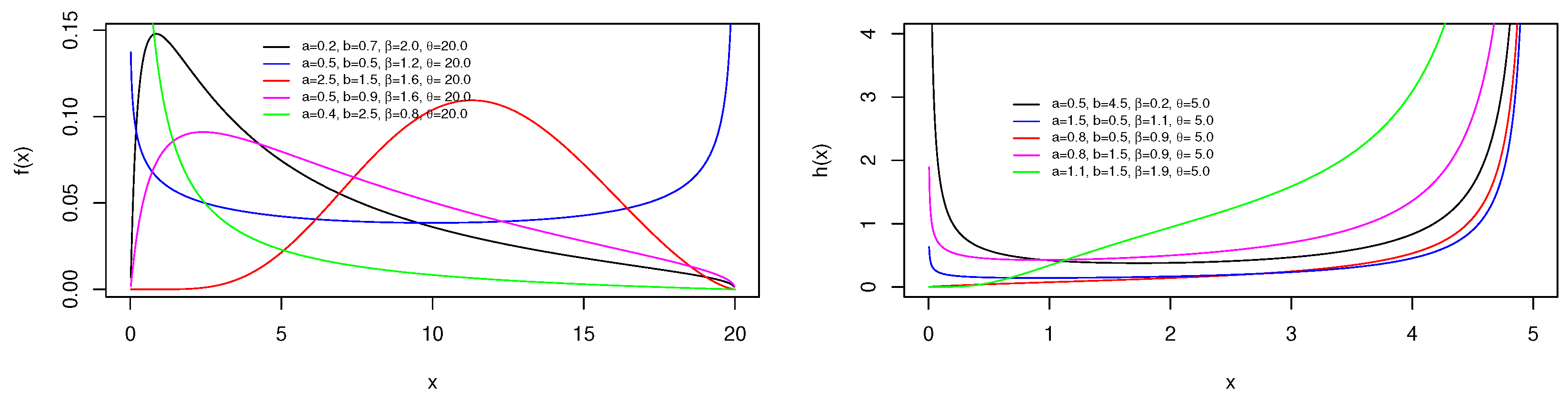
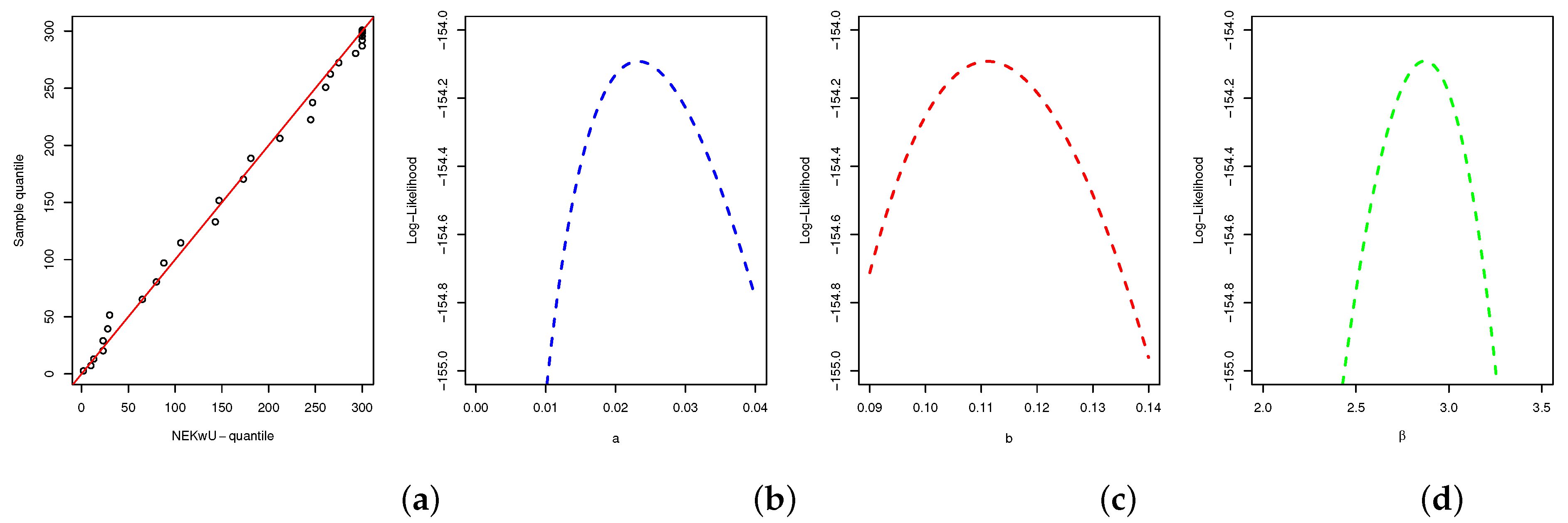
2.2.1. New Extended Kw Uniform (NEKwU) Distribution

To begin, we select the baseline uniform distribution U ( 0 , θ ) , with  θ > 0 . Its cdf and pdf are defined by G ( x ; θ ) = x / θ and g ( x ; θ ) = 1 / θ for x ( 0 , θ ) , respectively. We complete these definitions by G ( x ; θ ) = g ( x ; θ ) = 0 for x 0 , and  G ( x ; θ ) = 1 for x θ . By substituting these baseline functions into the cdf and pdf of the NEKwG family, we define the NEKwU distribution. Thus, the related pdf and hrf are specified by
f ( x ) = a b β 1 x log x θ β 1 e a ( log ( x / θ ) ) β 1 e a ( log ( x / θ ) ) β b 1
and
h ( x ) = a b β ( log ( x / θ ) ) β 1 e a ( log ( x / θ ) ) β x 1 e a ( log ( x / θ ) ) β , x ( 0 , θ ) , β , θ , a , b > 0 ,
respectively. It is understood that f ( x ) = h ( x ) = 0 for x ( 0 , θ ) .
Figure 1 shows a sample of plots of these functions for some parameter values.
We see in Figure 1 that the NEKwU distribution is flexible in terms of pdf and hrf curvatures. In particular, the pdf may have decreasing, unimodal right-skewed, unimodal near-symmetrical, and U shapes. These properties are generally desirable to model lifetime phenomena with such bounded value characteristics.
We finally mention the qf of the NEKwU distribution; based on Equation (5) and the qf of the considered uniform distribution, it is given by
Q ( u ) = θ e log 1 ( 1 u ) 1 / b / a 1 / β , u ( 0 , 1 ) .
With this function, quantile measures and functions are quite manageable.

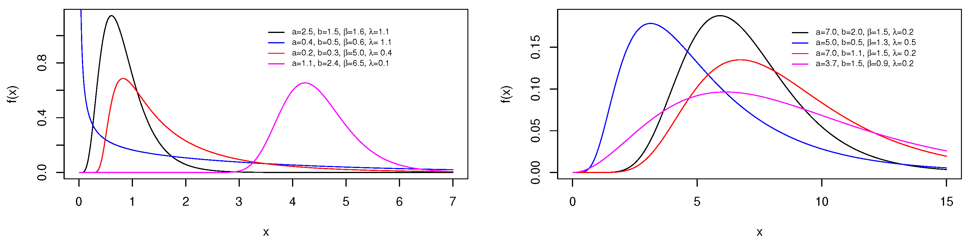
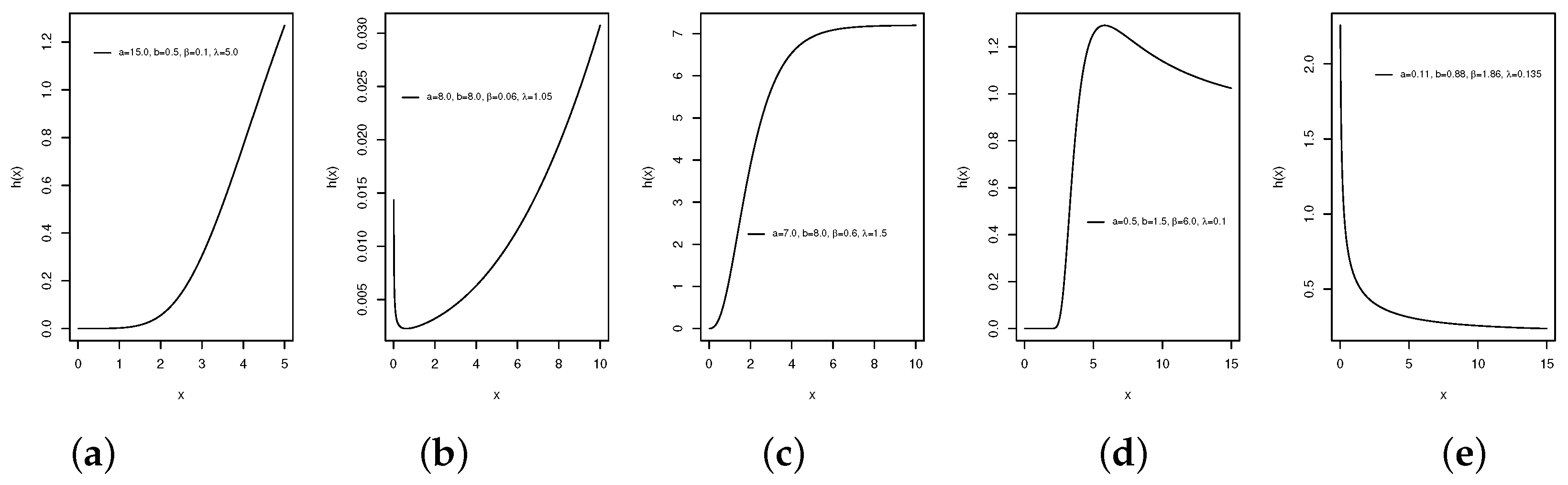
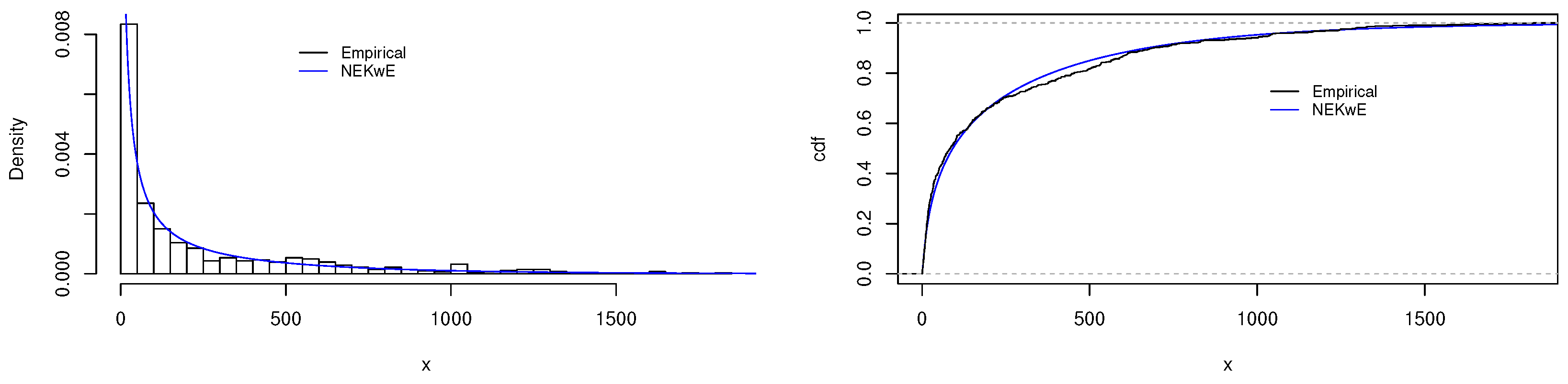
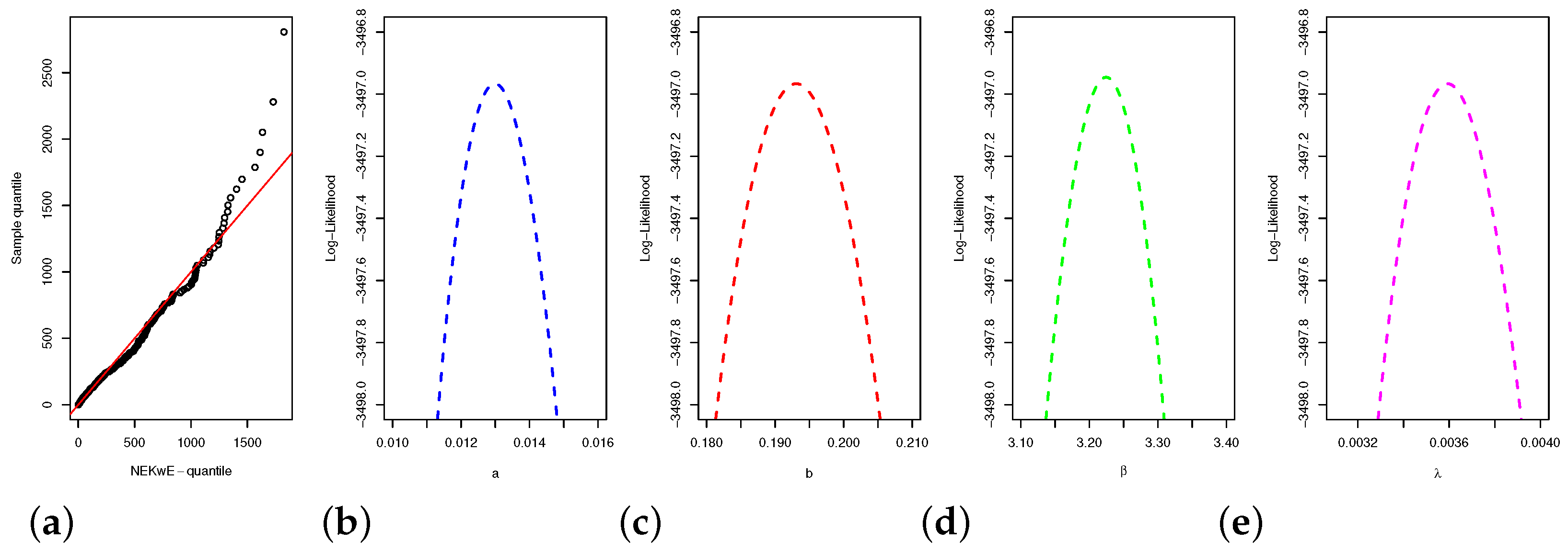
2.2.2. New Extended Kw Exponential (NEKwE) Distribution

For the second member of the NEKwG family, we consider the classical exponential distribution E ( λ ) , with  λ > 0 . Its cdf and pdf are defined by G ( x ; λ ) = 1 e λ x and g ( x ; λ ) = λ e λ x , respectively, for  x > 0 , and  G ( x ; λ ) = g ( x ; λ ) = 0 for x 0 . By substituting these baseline functions into the cdf and pdf of the NEKwG family, we define the NEKwE distribution. The related pdf and hrf are specified by
f ( x ) = a b β λ e λ x 1 e λ x log 1 e λ x β 1 e a log 1 e λ x β 1 e a ( log 1 e λ x ) β b 1
and
h ( x ) = a b β e λ x log 1 e λ x β 1 e a log 1 e λ x β 1 e λ x 1 e a log 1 e λ x β , x , β , λ , a , b > 0 ,
respectively. It is understood that f ( x ) = h ( x ) = 0 for x 0 . Figure 2 shows a sample of plots of the pdf, whereas Figure 3 isolates reachable shapes of the hrf of the NEKwE distribution for some parameter values.
We see in Figure 2 that the pdf is versatile in functionality, with diverse decreasing and unimodal, right-skewed, and near-symmetrical shapes.
The panel of hrf shapes displayed in Figure 3 reveals the high modeling power of the NEKwE distribution. Thus, it is perfect to model lifetime data of all nature. This aspect will be illustrated with an appropriate data set in the application section.
By using Equation (5) and the qf of the considered exponential distribution, the qf of the NEKwE distribution is obtained as
Q ( u ) = 1 λ log 1 e 1 a log 1 ( 1 u ) 1 / b 1 / β , u ( 0 , 1 ) .
Quantile measures and functions, as well as simulation studies based on the NEKwE distribution, are simple to use with this function.

3. Mathematical Developments

In this part, we examine some specific properties of the NEKwG family. We adopt the same mathematical concepts as those used in [48].

3.1. Asymptotic Results

To begin, some asymptotic results on the main related function are described in the next result.
Lemma 1.
The equivalence functions of the cdf, pdf, sf, and hrf of the NEKwG family are described below, by distinguishing whether G ( x ; η ) 0 or G ( x ; η ) 1 .
  • As G ( x ; η ) 0 , we have
    F ( x ) b e a G ( x ; η ) β , f ( x ) a b β g ( x ; η ) G ( x ; η ) G ( x ; η ) β 1 e a G ( x ; η ) β , h ( x ) a b β g ( x ; η ) G ( x ; η ) G ( x ; η ) β 1 e a G ( x ; η ) β .
  • As G ( x ; η ) 1 , we have
    s ( x ) a b G ( x ; η ) b β a b ( 1 G ( x ; η ) ) b β , f ( x ) a b b β g ( x ; η ) ( 1 G ( x ; η ) ) b β 1 , h ( x ) b β h G ( x ; η ) ,
    where h G ( x ; η ) denotes the hrf associated to the baseline distribution.
The proof is based on standard asymptotic equivalence results (see [49] (p. 10) and [50] (chap. 2)) that involve exponential functions of some expressions and verify by L’Hôpital’s rule. It is thus omitted. Similar properties were derived for the new extended Topp–Leone family in [41].
The preceding result is critical for understanding the role of the parameters a, b, and  β at the support boundaries of the baseline distribution. We see how a activates the exponential term, as well as how b and β affect baseline-type function exponentiation.

3.2. Expansions and Approximations

A pdf’s series representation simplifies the computation of some distributional properties. The result below explores this aspect for the exponentiated pdf of the NEKwG family.
Lemma 2.
Let ξ > 0 . Then we can express f ( x ) ξ as
f ( x ) ξ = i , j = 0 ϕ i , j ( ξ ) ψ j ( x ; β , ξ , η ) ,
where
ϕ i , j ( ξ ) = ( a b β ) ξ ( 1 ) i + j a j ( i + ξ ) j j ! ξ ( b 1 ) i
and
ψ j ( x ; β , ξ , η ) = g ( x ; η ) ξ G ( x ; η ) ξ G ( x ; η ) β ( j + ξ ) ξ .
Proof. 
By applying the generalized version of the binomial theorem in (2), followed by the exponential series expansion, we have
f ( x ) ξ = ( a b β ) ξ g ( x ; η ) ξ G ( x ; η ) ξ G ( x ; η ) ξ ( β 1 ) e a ξ G ( x ; η ) β 1 e a G ( x ; η ) β ξ ( b 1 ) = ( a b β ) ξ g ( x ; η ) ξ G ( x ; η ) ξ G ( x ; η ) ξ ( β 1 ) i = 0 ξ ( b 1 ) i ( 1 ) i e a ( i + ξ ) G ( x ; η ) β = ( a b β ) ξ g ( x ; η ) ξ G ( x ; η ) ξ G ( x ; η ) ξ ( β 1 ) i = 0 ξ ( b 1 ) i ( 1 ) i j = 0 ( 1 ) j a j ( i + ξ ) j j ! G ( x ; η ) β j = i , j = 0 ( a b β ) ξ ( 1 ) i + j a j ( i + ξ ) j j ! ξ ( b 1 ) i g ( x ; η ) ξ G ( x ; η ) ξ G ( x ; η ) β ( j + ξ ) ξ = i , j = 0 ϕ i , j ( ξ ) ψ j ( x ; β , ξ , η ) .
The proof ends.    □
As consequences of Lemma 2, several important moment-type measures of the NEKwG family can have a series expansion, or approximation.

3.3. Moments and Entropy

The r t h central moments and incomplete moments representations, as well as the Rényi entropy of the NEKwG family, are provided.
  • Moments are significant theoretical measures because they provide an alternative way to fully and uniquely specify a characteristic of a probability distribution, such as the central tendency, deviations, skewness, and kurtosis. Incomplete moments aid in obtaining mean deviations and some important reliability measures, such as moments of residual life. Let X be a random variable (rv) with a distribution belonging to the KwG family.
    • The r t h central moment of X can be expressed and approximated as
      m r = E ( X r ) = x r f ( x ) d x i , j = 0 M ϕ i , j ( 1 ) x r ψ j ( x ; β , 1 , η ) d x .
      From it, we can derive the mean ( E ( X ) ), variance ( v a r = E ( X 2 ) [ E ( X ) ] 2 ), and other raw-moment composed measures.
    • The r t h incomplete moment of X can be expressed and approximated as
      m r ( t ) = E ( X r 1 X < t ) = t x r f ( x ) d x i , j = 0 M ϕ i , j ( 1 ) t x r ψ j ( x ; β , 1 , η ) d x .
      Based on it, we can derive various mean deviations and reverse residual life functions.
    Remark 1.
    In the special case where β is an integer greater to 1 (implying that β ( j + 1 ) 1 is a positive integer for any positive integer j), we can express G ( x ; η ) β ( j + 1 ) 1 in a series form to further express ψ j ( x ; β , 1 , η ) . This will allow us to obtain the mean, variance, and other possible moments in series form. The following lemma is required: logarithmic series representation.
    Lemma 3.
    [51]  For a given power series of the form k = 0 a k x k , let n be a positive integer, then,
    k = 0 a k x k n = k = 0 c k x k ,
    where c 0 = a 0 n , c m = 1 m a 0 j = 1 m ( j n m + j ) a j c m j for m 1 .
    Hence, we can write
    ( log G ( x ; η ) ) β ( j + 1 ) 1 = 1 + n = 0 w n ( G ( x ; η ) 1 ) n β ( j + 1 ) 1
    where w 0 = 1 and w n = ( 1 ) n / n for n 1 . Therefore, by the binomial formula, we have
    G ( x ; η ) β ( j + 1 ) 1 = 1 + k = 1 β ( j + 1 ) 1 β ( j + 1 ) 1 k n = 0 w n ( G ( x ; η ) 1 ) n k .
    By virtue of Lemma 3, we obtain
    G ( x ; η ) β ( j + 1 ) 1 = 1 + k = 1 β ( j + 1 ) 1 n = 0 β ( j + 1 ) 1 k z n ( G ( x ; η ) 1 ) n ,
    where z 0 = w 0 n and z m = [ 1 / ( m w 0 ) ] j = 1 m ( j k m + j ) w j z m j for m 1 . Thus,
    G ( x ; η ) β ( j + 1 ) 1 = 1 + k = 1 β ( j + 1 ) 1 n = 0 κ i , j , k , l , n G l ( x ; η ) ,
    where κ i , j , k , l , n = l = 0 n β ( j + 1 ) 1 k n l ( 1 ) n l z n . As a result, from (8) at ξ = 1 , f ( x ) can be expressed as
    f ( x ) = i , j = 0 ϕ i , j ( 1 ) g ( x ; η ) G ( x ; η ) + i , j = 0 κ i , j , k , l , n * g ( x ; η ) G l 1 ( x ; η ) ,
    where κ i , j , l , n * = k = 1 β ( j + 1 ) 1 n = 0 ϕ i , j ( 1 ) κ i , j , l , n . In particular, the  r t h moments of X can be expressed as
    m r = i , j = 0 ϕ i , j ( 1 ) x r g ( x ; η ) G 1 ( x ; η ) d x + i , j = 0 κ i , j , k , l , n * x r g ( x ; η ) G l 1 ( x ; η ) d x ,
    thus,
    m r = i , j = 0 ϕ i , j ( 1 ) x r g ( x ; η ) G 1 ( x ; η ) d x + i , j = 0 κ i , j , k , l , n * l 1 E l ( Y r ) ,
    where E l ( Y r ) is the r t h moment associated to a random variable Y that follows the exponentiated baseline distribution with cdf G l ( x ; η ) . In particular, for our proposed NEKwE and NEKwU distributions, the expression of E l ( Y r ) are available in [52,53], respectively; the computation of the first integral in (11) follow similar way to the E l ( Y r ) . In Table 2 and Table 3, we provide some possible numerical values of some moments from (9) computed using theintegratefunction inR3.5.3software [54].
  • Entropy in information theory is directly analogous to entropy in statistical thermodynamics. The average level of information or uncertainty in a random variable or system is defined as its entropy. One can see [55,56].
    Here, we discuss the Rényi entropy of the new model. The Rényi entropy can be derived from the following formula:
    R ( ρ ) = 1 1 ρ log E ( f ( X ) ρ 1 ) ,
    where ρ > 0 and ρ 1 , and we can approximate the expectation term as
    E ( f ( X ) ρ 1 ) = f ( x ) ρ d x i , j = 0 M ϕ i , j ( ρ ) ψ j ( x ; β , ρ , η ) d x .
    An approximation of R ( ρ ) follows by substitution. This entropy measures the amount of information contained in X. Another useful entropy, the Shannon entropy defined by E [ log f ( X ) ] , is a special case of the Rényi entropy when ρ 1 .
In Table 2 and Table 3, we provide some possible numerical values of the first six moments and Rényi entropy of the NEKwE and NEKwU distributions, respectively.
These tables validate the adaptability of the considered measures, demonstrating the flexibility of the moments and the uncertain nature of the considered distributions.

3.4. Order Statistics and Applications

We now investigate some distributional properties of the order statistics related to the NEKwG family. Given a random sample of size n denoted by X 1 , X 2 , , X n , i = 1 , 2 , , n . , the order statistics are the rvs X ( 1 ) , X ( 2 ) , , X ( n ) , defined in function of X 1 , X 2 , , X n , such that X ( 1 ) = inf ( X 1 , X 2 , , X n ) , X ( n ) = sup ( X 1 , X 2 , , X n ) , and P ( X ( 1 ) X ( 2 ) , X ( n ) ) = 1 .
Order statistics play a significant role in theoretical studies and practice, especially the minimum, maximum, range, and study of a particular X i . One can find records and the role of order statistics in [57]. Order statistics have a wide range of applications in various fields such as survival analysis, life testing, reliability, quality control, signal processing, classification analysis, and wireless communication (see [58,59]). In addition, applications of order statistics are in biomedical studies (see [60]); image processing, filtering theory, and order statistics filters representing a class of non-linear filters (see [61]); and sampling plans (see [62]).
Lemma 4.
If the distribution of X 1 belongs to the NEKwG family, then the pdf of X ( i ) can be written as a finite combination of pdfs of the NEKwG family.
Proof. 
By using a well-known result on the pdf of order statistics, the pdf of X ( i ) is given by
f ( i ) ( x ) = i n i f ( x ) F ( x ) i 1 s ( x ) n i .
It follows from the binomial formula that
f ( i ) ( x ) = i n i j = 0 i 1 i 1 j ( 1 ) j f ( x ) s ( x ) j + n i ,
and we have
f ( x ) s ( x ) j + n i = a b β g ( x ; η ) G ( x ; η ) G ( x ; η ) β 1 e a G ( x ; η ) β 1 e a G ( x ; η ) β b ( j + n i + 1 ) 1 = 1 j + n i + 1 f j ( x ) ,
where f j ( x ) denotes the pdf of the NEKwG family with parameters a, b ( j + n i + 1 ) and β . This ends the proof.    □
Lemma 4 may be useful to determine moment-type measures of X ( i ) based on those of the NEKwG family. In particular, the  r t h raw moment of X ( i ) can be expressed as
m r , ( i ) = E ( X ( i ) r ) = j = 0 i 1 υ i , j m r , i , j * ,
where
υ j = i n i i 1 j ( 1 ) j 1 j + n i + 1
and m r , i , j * denotes the r t h raw moment of a rv with distribution belonging to the NEKwG family with parameters a, b ( j + n i + 1 ) , and β .
We now provide some asymptotic distribution results for the extreme order statistics in the special case of the NEKwE distribution for X 1 . On this topic, the general theory can be found in [63], among others.
Proposition 1.
Assume that X 1 follows the NEKwE distribution. Then, the sequence of rvs ( B n ) n 1 , where B n = ( X n : n a n ) / b n , a n = Q ( 1 1 / n ) and b n = E ( X 1 a n | X 1 a n ) , tends in distribution to a standard Gumbel distribution.
Proof. 
We aim to apply the result in [63] (Theorem 8.3.2). In this regard, we consider the following limit:
u ( x ) = lim t s ( t + x M ( t ) ) s ( t ) ,
where s ( t ) denotes the sf of the NEKwE distribution and M ( t ) = E ( X 1 t | X 1 t ) . As  x , we have
s ( x ) = 1 e a log 1 e λ x β b a b log 1 e λ x b β a b e λ b β x .
Hence, as  t , we have
M ( t ) = 0 s ( x + t ) s ( t ) d x 0 e λ b β x d x = 1 λ β b .
Therefore,
u ( x ) lim t e λ β b t + x / λ β b e λ β b t = e x .
The direct application in [63] (Theorem 8.3.2) yields the desired result.    □
The asymptotic distribution for X ( 1 ) is established in the next result.
Proposition 2.
Assume that X 1 follows the NEKwE distribution defined with β = 1 . Then, as  a , the sequence of rvs ( B n * ) n 1 , where B n * = ( X ( 1 ) a n * ) / b n * , a n * = Q ( 1 / n ) and b n * = E ( a n * X 1 | X 1 a n * ) , tends in distribution to the distribution of the rv log ( Y ) , where Y follows the standard exponential distribution.
Proof. 
We aim to use the result in [63] (Theorem 8.3.6). In this regard, we consider
v ( x ) = lim t 0 F ( t + x m ( t ) ) F ( t ) ,
where m ( t ) = E ( t X 1 | X 1 t ) and F ( t ) is the cdf of the NEKwE distribution defined with β = 1 . As  x 0 , we have
F ( x ) b e a log 1 e λ x b λ a x a .
Thus, as  t 0 , we have
m ( t ) = 0 t F ( x ) F ( t ) d x t a 0 t x a d x = t a + 1 .
Therefore, as  a ,
u ( x ) lim t b λ a ( t + t x / ( a + 1 ) ) a b λ t a = 1 + x a + 1 a e x .
The desired result is obtained by applying the result in [63] (Theorem 8.3.6) directly.    □

4. Inference

Maximum likelihood estimation, least-squares estimation, and Bayes estimation methods under the square error loss function are considered for estimating the parameters of the NEKwG models based on data. Additionally, their performance is studied using a simulation work. Once the estimates are obtained, function estimation can be derived through the plug-in method.

4.1. Maximum Likelihood Estimation Method

Maximum likelihood estimation is the most commonly used method in statistical inferences (see [64]). It is effective due to its advantages in theoretical studies and asymptotic efficiency. The authors of [65] provide a comprehensive note regarding this method. Let X 1 , X 2 , , X n be a random sample of size n from the NEKwG distribution with unknown parameters and  x 1 , x 2 , , x n be associated observations. Let Θ = ( β , a , b , η ) T be the vector of these parameters. The maximum likelihood estimates (MLEs) of the parameters in Θ , constituting the MLE vector Θ ^ = ( β ^ , a ^ , b ^ , η ^ ) T , can be computed by maximization of the following function with respect to Θ , called the log-likelihood function:
( Θ ) = i = 1 n log f ( x i ) = n log a + n log b + n log β + i = 1 n log g ( x i ; η ) i = 1 n log G ( x i ; η ) + ( β 1 ) i = 1 n log G ( x i ; η ) a i = 1 n G ( x i ; η ) β + ( b 1 ) i = 1 n log 1 e a G ( x i ; η ) β .
The MLEs of the parameters are also the solutions of the following equations:
( Θ ) a = n a i = 1 n G ( x i ; η ) β + ( b 1 ) i = 1 n G ( x i ; η ) β e a G ( x i ; η ) β 1 e a G ( x i ; η ) β = 0 , ( Θ ) b = n b + i = 1 n log 1 e a G ( x i ; η ) β = 0 , ( Θ ) β = n β + i = 1 n log G ( x i ; η ) a i = 1 n G ( x i ; η ) β log G ( x ; η ) + a ( b 1 ) i = 1 n G ( x i ; η ) β log G ( x i ; η ) e a G ( x i ; η ) β 1 e a G ( x i ; η ) β = 0
and
( Θ ) η = i = 1 n g η ( x i ; η ) g ( x i ; η ) i = 1 n G η ( x i ; η ) G ( x i ; η ) + ( β 1 ) i = 1 n G η ( x i ; η ) G ( x i ; η ) log G ( x i ; η ) + a β i = 1 n G η ( x i ; η ) G ( x i ; η ) β 1 G ( x i ; η ) a β ( b 1 ) i = 1 n G η ( x i ; η ) G ( x i ; η ) β 1 e a G ( x i ; η ) β 1 e a G ( x i ; η ) β G ( x i ; η ) = 0 ,
where g η ( x i ; η ) and G η ( x i ; η ) denote the partial derivative of g ( x i ; η ) and G ( x i ; η ) , respectively, with respect to the parameter vector η .
The theory underlying the MLEs is well known and can be applied to perform a more detailed estimated analysis of the parameters. If n is large enough, the asymptotic distribution of the vector of MLEs is a multivariate normal distribution with the same dimension as the total number of unknown parameters, zero mean, and a well-identified variance–covariance matrix. We can derive the standard errors (SEs) of the MLEs, as well as confidence intervals and ratio likelihood tests.

4.2. Least-Squares Estimation Method

Under the statistical setting of the above part, let us now consider the ordered observations denoted by x ( 1 ) , x ( 2 ) , , x ( n ) . One of the oldest methods of estimation is the least-squares estimation (see [66]); for many decades this method was used to estimate the parameters of beta distributions (see [67]). The least-squares estimates (LSEs) of the parameters in Θ , constituting the LSE vector Θ ^ = ( β ^ , a ^ , b ^ , η ^ ) T , can be computed by minimizing the least-squares function with respect to Θ , called the least-squares function:
L ( Θ ) = i = 1 n F ( x ( i ) ) i n + 1 2 = i = 1 n n + 1 i n + 1 1 e a G ( x ( i ) ; η ) β b 2 ,
These LSEs of the parameters are also the solutions of the following equations:
L ( Θ ) a = 2 b i = 1 n 1 1 δ ( x ( i ) ; a , β , η ) b i n + 1 × δ ( x ( i ) ; a , β , η ) G ( x ( i ) ; η ) β 1 δ ( x ( i ) ; a , β , η ) b 1 = 0 , L ( Θ ) b = 2 i = 1 n 1 1 δ ( x ( i ) ; a , β , η ) b i n + 1 × 1 δ ( x ( i ) ; a , β , η ) b 1 log 1 δ ( x ( i ) ; a , β , η ) = 0 , L ( Θ ) β = 2 a b i = 1 n 1 1 δ ( x ( i ) ; a , β , η ) b i n + 1 × δ ( x ( i ) ; a , β , η ) G ( x ( i ) ; η ) β log G ( x ( i ) ; η ) 1 δ ( x ( i ) ; a , β , η ) b 1 = 0
and
L ( Θ ) η = 2 a b β i = 1 n 1 1 δ ( x ( i ) ; a , β , η ) b i n + 1 δ ( x ( i ) ; a , β , η ) G η ( x ( i ) , η ) G ( x ( i ) ; η ) × G ( x ( i ) ; η ) β 1 1 δ ( x ( i ) ; a , β , η ) b 1 = 0 ,
where δ ( x i ; a , β , η ) = e a G ( x ( i ) ; η ) β .

4.3. Bayes Estimation Method

Bayesian procedures for estimating parameters have been successfully applied in various situations and many disciplines, for instance, in physics (see [68]), epidemiology (see [69]), and econometrics (see [70]). One of the advantages of Bayesian methods is that they allow estimating models when traditional estimation fails due to model complexity. We now discuss the Bayes estimation of Θ under the square error loss (SEL) function. The Bayes estimates (BEs) of the parameters in Θ , constituting the BE vector Θ ^ = ( β ^ , a ^ , b ^ , η ^ ) T , are derived from the posterior distributions given the data. A brief description of the method is proposed below. Let N and K be the number of iterations and burn in samples, respectively. Then, the SEL function for the assumed prior distribution is minimized by the posterior mean as
Θ ^ = 1 N K i = K + 1 N Θ ^ ( i ) ,
where Θ ^ ( i ) refers to the MLE vector of Θ at the i t h iteration. Furthermore, we can establish the highest posterior density (HPD) credible interval for Θ ^ using the package HDInterval elaborated in [71] in the R software.
Now, let X 1 , X 2 , , X n be a random sample of size n drawn from a general distribution of the NEKwG family with unknown parameters, and  x 1 , x 2 , , x n represent associated observations. We suppose that η contains m 3 unknown parameters, such as η = ( η 4 , η 5 , , η m ) and turn out β , a , b , and η as independent rvs that follow the gamma distribution with the pdf defined by
ȷ j ( x ) = d j c j Γ ( c j ) x c j 1 e d j x , x > 0 ,
j = 1 , 2 , 3 , , m , respectively, and  ȷ j ( x ) = 0 for x 0 . Here, Γ ( c ) denotes the standard gamma function. In this context, the related likelihood function is specified by
( Θ | d a t a ) = a n b n β n i = 1 n g ( x i ; η ) i = 1 n G 1 ( x i ; η ) i = 1 n G ( x i ; η ) β 1 e a i = 1 n G ( x i ; η ) β × i = 1 n 1 e a G ( x i ; η ) β b 1 .
The joint posterior pdf of Θ | d a t a can be derived as
π ( Θ | d a t a ) = ( Θ | d a t a ) ȷ j ( Θ ) z ( d a t a ; Θ ) d Θ ,
where z ( d a t a ; Θ ) = ( Θ | d a t a ) ȷ j ( Θ ) is the joint pdf for the data. The conditional posterior pdfs of β , a , b , and η can be derived from Equation (14) as
π 1 ( a ) a n + c 1 1 e a i = 1 n G ( x i ; η ) β d 1 a i = 1 n 1 e a G ( x i ; η ) β b 1 ,
π 2 ( b ) b n + c 2 1 e d 2 b i = 1 n 1 e a G ( x i ; η ) β b 1 ,
π 3 ( β ) β n + c 3 1 e a i = 1 n G ( x i ; η ) β d 3 β i = 1 n G ( x i ; η ) β 1 i = 1 n 1 e a G ( x i ; η ) β b 1 ,
and, for  j = 4 , , m ,
π j ( η ) η j c j 1 e a i = 1 n G ( x i ; η j ) β d j η j i = 1 n g ( x i ; η j ) i = 1 n G 1 ( x i ; η j ) i = 1 n G ( x i ; η j ) β 1 × i = 1 n 1 e a G ( x i ; η j ) β b 1 .
Since none of these posterior pdfs correspond to a common distribution, we can apply the Metropolis–Hastings algorithm (MHA) and the Gibbs sampling technique to generate samples from the posterior distributions. Further details in this regard can be found in [72,73,74]. The MHA uses the normal distribution as a proposal distribution. The step-by-step instructions are provided below, taking the Gibbs sampling technique into account:
(i)
Begin with initial values ( a ( 0 ) , b ( 0 ) , β ( 0 ) , η ( 0 ) ) ;
(ii)
Set t = 1 ;
(iii)
Apply the MHA to generate a ( t ) from π 1 ( a ) in (15);
(iv)
Apply the MHA to generate b ( t ) from π 2 ( b ) in ();
(v)
Apply the MHA to generate β ( t ) from π 3 ( β ) in ();
(vi)
Apply the MHA to generate η j ( t ) from π j ( η ) in (18);
(vii)
Set t = t + 1 ;
(viii)
Repeat the procedures in (iii) to (vii) T times.
For a large-enough T, Θ ^ can be obtained based on the SEL function. Furthermore, an approximate 100 ( 1 ϵ ) % HPD credible interval of Θ can be established using the procedure given in [75]. In the next subsection, we will choose some value of T to demonstrate how the technique works on our models. In some particular problems, practitioners have provided some ways of determining T based on their studies, we referred to the last paragraph in [76] (Section 4).

4.4. Simulation

Simulation studies are computer experiments that involve creating data by pseudo-random sampling. A strong point of simulation studies is the ability to comprehend the behavior of statistical methods because some facts, say, parameters, are known from the process of generating the data. This allows us to consider properties of methods, such as bias, standard deviation, etc.; one can see [77].
A simulation study was conducted to discuss the performance of the maximum likelihood, least-squares, and Bayes estimation methods as described above, using the R3.5.3 software (see [54]) for the special NEKwE distribution. In this regard, M = 1000 moderate samples, each of size n = ( 30 , 60 , 90 , , 300 ) , is generated from the NEKwE distribution for selected parameter values. For the Bayes estimation, we use T = 1000 iterations and the first 20 % as burn-in samples. We also discover that when the hyperparameters are set to greater than one, they work well. In this case, we consider c 1 = 9 , d 1 = 6 , c 2 = 9 , d 2 = 6 , c 3 = 9 , d 3 = 5 , c 4 = 5 , and d 4 = 6 . The bias and mean square error (MSE) of the estimates are examined. Table 4 and Table 5 show the simulation findings, including the average estimate (AE). We provide some important steps for the numerical simulation below:
  • Choose the sample size n, replication number M, and the values of parameters a , b , β , η ;
  • Generate random sample with U i following the uniform ( 0 , 1 ) distribution, i = 1 , 2 , 3 , n ;
  • Generate random sample with X i following the NEKwE distribution, i = 1 , 2 , 3 , n , from (7);
  • Calculate the MLEs, LSEs, and BEs of the parameters of the NEKwE distribution from the simulated data;
  • Repeat steps 2 4 , M times;
  • Calculate the average bias and the average MSE for each parameter.
From Table 4 and Table 5, we can see that the MLEs, LSEs, and BEs perform consistently, that the MSEs of the estimates decrease as the sample size increases, and that the bias is sometimes negative. As a result, the related approaches can be deemed effective in estimating the parameters of the NEKwE distribution, as well as those of the other NEKwG family members.

5. Real Data Illustrations

Using two real data studies, this section compares the flexibility and advantages of the models generated by the NEKwG family to those generated by other popular families. To be more specific, the NEKwE and NEKwU models are considered under two different data analysis scenarios. We compare the performance of the models in terms of fit using the Akaike information criterion (AIC), Bayesian information criterion (BIC), Corrected AIC (CAIC), Kolmogorov–Smirnov (KS), Anderson–Darling (AD), and Cramér–von Mises (CvM). As with the numerical values of the AIC, BIC, and CAIC, the estimated maximum likelihood function (L) is also computed. The distribution with the smallest value among these measures represents the data better than the others.
The considered competing models are listed as follows: Weibull–Pareto (WP) model (see [78]), transmuted exponentiated U-quadratic (TEUq) model (see [79]), Kw exponentiated U-quadratic (KwEUq) model (see [80]), modified Weibull (MW) model (see [81]), flexible Weibull (FW) model (see [82]), Kw-power (KwP) model (see [83]), Poisson-odd-exponential uniform (POEU) model (see [84]), beta uniform (BU) model (see [85]), exponentiated Kw-power (EKwP) model (see [86]), beta exponential (BE) model (see [87]), beta generalized exponential (BGE) model (see [88]), beta Erlang-truncated exponential (BETE) model (see [89]), generalized exponential Poisson (GEP) model (see [90]), generalized exponential (GE) model (see [52]), exponentiated Nadarajah and Haghighi (ENH) model (see [91,92]), extended Erlang-truncated exponential (EETE) model (see [93]), Kw half-logistic (KwHL) model (see [94]), Kw exponential (KwE) model (see [95]), Kw Weibull (KwW) model (see [96]), extended cosine exponential (ExCE) model (see [48]), exponentiated sine exponential (ESE) model (see [97]), exponentiated Kw exponential (EKwE) model, and exponentiated Kw Weibull (EKwE) model (see [29]).

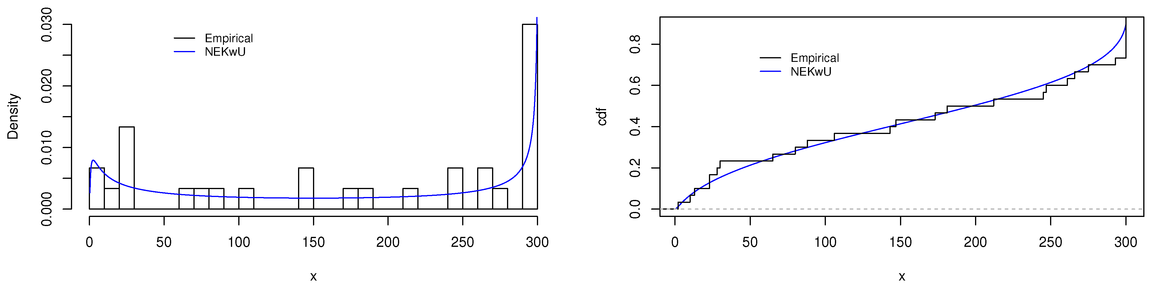
5.1. First Data Illustration

The first data set is reported from [98]. The values are the failure and run times from a sample of 30 devices: 2, 10, 13, 23, 23, 28, 30, 65, 80, 88, 106, 143, 147, 173, 181, 212, 245, 247, 261, 266, 275, 293, 300, 300, 300, 300, 300, 300, 300, 300. The numerical results of the estimates and goodness of fit measures of the competing models for the first data are given in Table 6 and Table 7. The results obtained based on the six goodness of fits in Table 7 indicate that the NEKwU model has the least numerical values, thus representing the data better than the other competing models, including some of the more popular Kw generated models with respect to uniform distribution. Importantly, note that Figure 4 shows how well the plots of the histogram of the first data are fitted by the NEKwU pdf and how well the empirical cdf is fitted by the NEKwU cdf. In particular, from Figure 4 (left), it is clear that the fitted NEKwU pdf has well captured the special U-shape of the histogram, and the data at the boundaries have also been properly fitted. Figure 5a shows the quantile–quantile (QQ) plot of the NEKwU model to visually check the data adequacy and its relatedness. In addition, Figure 5b–d are the plots of the profile log-likelihood functions to present the uniqueness of the obtained MLEs.

5.2. Second Data Illustration

Here, we want to display how the new families can perform well when dealing with COVID-19 data. The second data set is the number of daily new deaths caused by COVID-19 in the UK from 15 February 2020 to 7 September 2021. The data were extracted from the following internet link: https://www.worldometers.info/coronavirus/country/uk/ accessed on 3 September 2022: 1, 1, 1, 4, 2, 1, 18, 14, 22, 15, 33, 42, 32, 54, 24, 67, 143, 178, 226, 283, 294, 214, 375, 383, 662, 641, 735, 761, 645, 568, 1040, 1035, 1109, 1152, 840, 685, 745, 1044, 841, 1031, 937, 1111, 495, 557, 1169, 824, 719, 1004, 832, 405, 320, 903, 768, 658, 710, 588, 291, 278, 677, 612, 493, 590, 289, 241, 194, 564, 444, 377, 328, 428, 100, 150, 473, 309, 284, 308, 230, 387, 103, 124, 426, 345, 270, 149, 73, 94, 237, 249, 139, 253, 151, 61, 47, 188, 159, 82, 133, 104, 33, 30, 114, 106, 75, 79, 75, 34, 14, 89, 87, 102, 78, 40, 31, 21, 51, 99, 40, 48, 35, 19, 11, 53, 57, 32, 34, 17, 9, 8, 46, 26, 23, 27, 9, 11, 10, 25, 17, 9, 32, 15, 8, 3, 21, 34, 2, 18, 13, 5, 1, 18, 14, 18, 12, 3, 5, 17, 14, 20, 18, 11, 3, 5, 3, 12, 16, 6, 2, 18, 6, 4, 16, 16, 12, 9, 12, 1, 2, 3, 10, 13, 10, 12, 2, 3, 32, 8, 14, 6, 9, 5, 9, 27, 20, 21, 27, 27, 18, 11, 37, 37, 40, 35, 34, 17, 13, 71, 71, 59, 66, 49, 33, 19, 76, 70, 77, 87, 81, 65, 50, 143, 137, 138, 136, 150, 67, 80, 241, 191, 189, 224, 174, 151, 102, 368, 310, 280, 274, 326, 162, 136, 398, 493, 379, 356, 414, 156, 194, 533, 596, 564, 377, 463, 168, 213, 599, 530, 502, 511, 341, 399, 206, 608, 697, 498, 522, 480, 213, 205, 604, 649, 415, 505, 398, 231, 172, 617, 534, 517, 426, 520, 144, 232, 507, 613, 533, 490, 535, 326, 215, 692, 745, 575, 571, 241, 316, 402, 415, 983, 966, 614, 446, 455, 452, 831, 1044, 1165, 1328, 1038, 564, 530, 1246, 1567, 1251, 1283, 1298, 672, 600, 1613, 1824, 1293, 1404, 1351, 611, 593, 1634, 1729, 1242, 1248, 1203, 588, 407, 1452, 1325, 916, 1016, 829, 374, 333, 1055, 1003, 679, 759, 622, 258, 230, 800, 739, 455, 534, 446, 214, 178, 549, 443, 323, 346, 290, 144, 104, 343, 315, 242, 236, 158, 82, 65, 231, 190, 181, 175, 121, 52, 64, 110, 141, 94, 101, 96, 33, 17, 112, 98, 63, 70, 58, 19, 22, 56, 43, 51, 52, 10, 10, 26, 20, 45, 53, 60, 40, 7, 13, 23, 38, 30, 34, 35, 10, 4, 31, 22, 18, 40, 32, 11, 6, 17, 29, 22, 15, 7, 14, 1, 4, 27, 13, 15, 5, 2, 4, 20, 11, 11, 17, 7, 4, 5, 7, 3, 7, 9, 6, 5, 3, 15, 9, 10, 10, 7, 6, 1, 12, 18, 11, 13, 4, 1, 13, 6, 7, 17, 12, 8, 3, 10, 9, 19, 11, 14, 6, 5, 27, 19, 21, 18, 23, 11, 3, 23, 14, 22, 27, 18, 15, 9, 37, 33, 35, 29, 34, 26, 6, 50, 49, 63, 49, 41, 25, 19, 96, 73, 84, 64, 86, 28, 14, 131, 91, 85, 68, 71, 65, 24, 138, 119, 86, 92, 103, 39, 37, 146, 104, 94, 100, 91, 61, 26, 170, 111, 113, 114, 104, 49, 40, 174, 149, 140, 100, 133, 61, 48, 50, 207, 178, 121, 120, 68, 45, 209, 191, 167, 147, 156, 56, 61, 185, 201, 158, 178, 164.
The computed numerical results of the estimates and six goodness-of-fit measures for the second data set are provided in Table 8 and Table 9, respectively. The results show that the NEKwE model fit the data better than the other competing models because it has the lowest values for all model selection measures: AIC = 7001.93 , BIC = 7019.24 , CAIC = 7002.01 , KS = 0.0483 , AD = 1.3119 , and CvM = 0.2142 . Based on these data, the NEKwE model outperforms many popular Kw and exponentially generated models, clearly outperforming those in Table 9. In support of that, Figure 6 shows how excellently the plots of the histogram of the second data are fitted by the NEKwE pdf and how well the empirical cdf is fitted by the NEKwE cdf. Based on Figure 6 (left), it is clear that the fitted NEKwE pdf has perfectly fitted the decreasing tendency of the histogram, importantly, the KS = 0.0483 , which is considerably very small. Figure 7a shows the QQ plot of the NEKwE model, illustrating that the quantiles are quite related. Finally, Figure 7b–d are the plots of the profile log-likelihood functions of the NEKwE model to show the uniqueness of the estimated MLEs.

6. Conclusions

In this research paper, we proposed a new extension of the Kumaraswamy generated (KwG) family of distributions, designated as the NEKwG family. The model has flexible members capable of fitting decreasing, increasing, unimodal, and bathtub failure rates. Some special members were presented and studied, namely, the new extended Kw uniform (NEKwU) and new extended Kw exponential (NEKwE) distributions. Several properties of the NEKwG family were established, such as closed-form expressions for the probability density function and its series representation, the cumulative distribution function, various moments, order statistic results, and Rényi entropy.
Maximum likelihood estimates, least-squares estimates, and Bayes estimates of the model parameters were examined. The simulation studies were carried out using the NEKwE model, which examined the mean square error and bias of the estimators from the three techniques. The simulation result was quite good, as both the MSEs of the estimates decreased as sample size increased. In addition, two real-world data illustrations were provided to demonstrate the flexibility of the fitted model and how they outperform other popular models in practice as measured by some model selection criteria and goodness-of-fit tests; one of the data sets is the number of daily new deaths due to COVID-19 in the UK from 15 February 2020 to 7 September 2021.
Finally, we recommend further analysis of the other models of the NEKwG family and their estimation methods, such as product spacing and percentile estimation methods, among others. Discrete versions or multivariate extensions are also interesting directions of research.

Author Contributions

Conceptualization, S.A., M.M., F.J., C.C., I.M. and M.B.; methodology, S.A., M.M., F.J., C.C., I.M. and M.B.; software, S.A., M.M., F.J., C.C., I.M. and M.B.; validation, S.A., M.M., F.J., C.C., I.M. and M.B.; formal analysis, S.A., M.M., F.J., C.C., I.M. and M.B.; investigation, S.A., M.M., F.J., C.C., I.M. and M.B.; resources, S.A., M.M., F.J., C.C., I.M. and M.B.; data curation, S.A., M.M., F.J., C.C., I.M. and M.B.; writing—original draft preparation, S.A., M.M., F.J., C.C., I.M. and M.B.; writing—review and editing, S.A., M.M., F.J., C.C., I.M. and M.B.; visualization, S.A., M.M., F.J., C.C., I.M. and M.B. All authors have read and agreed to the published version of the manuscript.

Funding

This research received no external funding.

Institutional Review Board Statement

Not applicable.

Informed Consent Statement

Not applicable.

Data Availability Statement

The data used in the article are given therein.

Conflicts of Interest

The authors declare no conflict of interest.

References

  1. Kumaraswamy, P. A generalized probability density function for double-bounded random processes. J. Hydrol. 1980, 46, 79–88. [Google Scholar] [CrossRef]
  2. Jones, M. Kumaraswamy’s distribution: A beta-type distribution with some tractability advantages. Stat. Methodol. 2009, 6, 70–81. [Google Scholar] [CrossRef]
  3. Ponnambalam, K.; Seifi, A.; Vlach, J. Probabilistic design of systems with general distributions of parameters. Int. J. Circuit Theory Appl. 2001, 29, 527–536. [Google Scholar] [CrossRef]
  4. Nadarajah, S. On the distribution of Kumaraswamy. J. Hydrol. 2008, 348, 568–569. [Google Scholar] [CrossRef]
  5. Mitnik, P.A.; Baek, S. The Kumaraswamy distribution: Median-dispersion re-parameterizations for regression modeling and simulation-based estimation. Stat. Pap. 2013, 54, 177–192. [Google Scholar] [CrossRef]
  6. Pumi, G.; Rauber, C.; Bayer, F.M. Kumaraswamy regression model with Aranda-Ordaz link function. Test 2020, 29, 1051–1071. [Google Scholar] [CrossRef]
  7. Hamedi-Shahraki, S.; Rasekhi, A.; Yekaninejad, M.S.; Eshraghian, M.R.; Pakpour, A.H. Kumaraswamy regression modeling for Bounded Outcome Scores. Pak. J. Stat. Oper. Res. 2021, 17, 79–88. [Google Scholar] [CrossRef]
  8. Sundar, V.; Subbiah, K. Application of double bounded probability density function for analysis of ocean waves. Ocean Eng. 1989, 16, 193–200. [Google Scholar] [CrossRef]
  9. Seifi, A.; Ponnambalam, K.; Vlach, J. Maximization of manufacturing yield of systems with arbitrary distributions of component values. Ann. Oper. Res. 2000, 99, 373–383. [Google Scholar] [CrossRef]
  10. Fletcher, S.; Ponnambalam, K. Estimation of reservoir yield and storage distribution using moments analysis. J. Hydrol. 1996, 182, 259–275. [Google Scholar] [CrossRef]
  11. Ganji, A.; Ponnambalam, K.; Khalili, D.; Karamouz, M. Grain yield reliability analysis with crop water demand uncertainty. Stoch. Environ. Res. Risk Assess. 2006, 20, 259–277. [Google Scholar] [CrossRef]
  12. Garg, M. On Generalized Order Statistics From Kumaraswamy Distribution. Tamsui Oxf. J. Math. Sci. (TOJMS) 2009, 25, 153–166. [Google Scholar]
  13. Lemonte, A.J. Improved point estimation for the Kumaraswamy distribution. J. Stat. Comput. Simul. 2011, 81, 1971–1982. [Google Scholar] [CrossRef]
  14. Gholizadeh, R.; Khalilpor, M.; Hadian, M. Bayesian estimations in the Kumaraswamy distribution under progressively type II censoring data. Int. J. Eng. Sci. Technol. 2011, 3, 47–65. [Google Scholar] [CrossRef]
  15. Sindhu, T.N.; Feroze, N.; Aslam, M. Bayesian analysis of the Kumaraswamy distribution under failure censoring sampling scheme. Int. J. Adv. Sci. Technol. 2013, 51, 39–58. [Google Scholar]
  16. Nadar, M.; Papadopoulos, A.; Kızılaslan, F. Statistical analysis for Kumaraswamy’s distribution based on record data. Stat. Pap. 2013, 54, 355–369. [Google Scholar] [CrossRef]
  17. Nadar, M.; Kızılaslan, F.; Papadopoulos, A. Classical and Bayesian estimation of P(Y<X) for Kumaraswamy’s distribution. J. Stat. Comput. Simul. 2014, 84, 1505–1529. [Google Scholar]
  18. Nadar, M.; Kızılaslan, F. Classical and Bayesian estimation of P(X<Y) using upper record values from Kumaraswamy’s distribution. Stat. Pap. 2014, 55, 751–783. [Google Scholar]
  19. Dey, S.; Mazucheli, J.; Nadarajah, S. Kumaraswamy distribution: Different methods of estimation. Comput. Appl. Math. 2018, 37, 2094–2111. [Google Scholar] [CrossRef]
  20. Ahmad, Z.; Hamedani, G.G.; Butt, N.S. Recent developments in distribution theory: A brief survey and some new generalized classes of distributions. Pak. J. Stat. Oper. Res. 2019, 15, 87–110. [Google Scholar] [CrossRef]
  21. Cordeiro, G.M.; de Castro, M. A new family of generalized distributions. J. Stat. Comput. Simul. 2011, 81, 883–898. [Google Scholar] [CrossRef]
  22. Ahmed, M.A.; Mahmoud, M.R.; ElSherbini, E.A. The new Kumaraswamy Kumaraswamy family of generalized distributions with application. Pak. J. Stat. Oper. Res. 2015, 11, 159–180. [Google Scholar] [CrossRef]
  23. Alizadeh, M.; Tahir, M.; Cordeiro, G.M.; Mansoor, M.; Zubair, M.; Hamedani, G. The Kumaraswamy Marshal-Olkin family of distributions. J. Egypt. Math. Soc. 2015, 23, 546–557. [Google Scholar] [CrossRef]
  24. Afifya, A.Z.; Cordeiro, G.M.; Yousof, H.M.; Nofal, Z.M.; Alzaatreh, A. The Kumaraswamy transmuted-G family of distributions: Properties and applications. J. Data Sci. 2016, 14, 245–270. [Google Scholar] [CrossRef]
  25. Hassan, A.S.; Elgarhy, M. Kumaraswamy Weibull-generated family of distributions with applications. Adv. Appl. Stat. 2016, 48, 205. [Google Scholar] [CrossRef]
  26. Chakraborty, S.; Handique, L. Properties and data modelling applications of the Kumaraswamy generalized Marshall-Olkin-G family of distributions. J. Data Sci. 2017, 605, 620. [Google Scholar] [CrossRef]
  27. Nofal, Z.M.; Altun, E.; Afify, A.Z.; Ahsanullah, M. The generalized Kumaraswamy-G family of distributions. J. Stat. Theory Appl. 2019, 18, 329–342. [Google Scholar] [CrossRef]
  28. El-Sherpieny, E.S.; Elsehetry, M. Kumaraswamy type I half logistic family of distributions with applications. Gazi Univ. J. Sci. 2019, 32, 333–349. [Google Scholar]
  29. Silva, R.; Gomes-Silva, F.; Ramos, M.; Cordeiro, G.; Marinho, P.; De Andrade, T.A. The exponentiated Kumaraswamy-G Class: General properties and application. Rev. Colomb. De Estadística 2019, 42, 1–33. [Google Scholar] [CrossRef]
  30. Tahir, M.H.; Hussain, M.A.; Cordeiro, G.M.; El-Morshedy, M.; Eliwa, M.S. A new Kumaraswamy generalized family of distributions with properties, applications, and bivariate extension. Mathematics 2020, 8, 1989. [Google Scholar] [CrossRef]
  31. Chakraborty, S.; Handique, L.; Jamal, F. The Kumaraswamy Poisson-G family of distribution: Its properties and applications. Ann. Data Sci. 2020, 9, 229–247. [Google Scholar] [CrossRef]
  32. El-Morshedy, M.; Tahir, M.H.; Hussain, M.A.; Al-Bossly, A.; Eliwa, M.S. A New Flexible Univariate and Bivariate Family of Distributions for Unit Interval (0, 1). Symmetry 2022, 14, 1040. [Google Scholar] [CrossRef]
  33. Ramos, M.W.A.; Marinho, P.R.D.; Cordeiro, G.M.; da Silva, R.V.; Hamedani, G. The Kumaraswamy-G Poisson family of distributions. J. Stat. Theory Appl. 2015, 14, 222–239. [Google Scholar] [CrossRef]
  34. Handique, L.; Chakraborty, S. A new beta generated Kumaraswamy Marshall-Olkin-G family of distributions with applications. Malays. J. Sci. 2017, 36, 157–174. [Google Scholar] [CrossRef]
  35. Handique, L.; Chakraborty, S. The Beta generalized Marshall-Olkin Kumaraswamy-G family of distributions with applications. Int. J. Agricult. Stat. Sci 2017, 13, 721–733. [Google Scholar]
  36. Handique, L.; Chakraborty, S.; Hamedani, G. The Marshall-Olkin-Kumaraswamy-G family of distributions. J. Stat. Theory Appl. 2017, 16, 427–447. [Google Scholar] [CrossRef] [Green Version]
  37. Handique, L.; Chakraborty, S.; Ali, M.M. Beta Generated Kumaraswamy-G Family of Distributions. Pak. J. Stat. 2017, 33, 467–490. [Google Scholar]
  38. Alshkaki, R. A generalized modification of the Kumaraswamy distribution for modeling and analyzing real-life data. Stat. Optim. Inf. Comput. 2020, 8, 521–548. [Google Scholar] [CrossRef]
  39. Selim, M.A. The Distributions of Beta-Generated and Kumaraswamy-Generalized Families: A Brief Survey. Figshare 2020, 1–19. [Google Scholar] [CrossRef]
  40. Muhammad, M.; Liu, L. A new extension of the beta generator of distributions. Math. Slovaca 2022, 72, 1319–1336. [Google Scholar] [CrossRef]
  41. Muhammad, M.; Liu, L.; Abba, B.; Muhammad, I.; Bouchane, M.; Zhang, H.; Musa, S. A New Extension of the Topp–Leone-Family of Models with Applications to Real Data. Ann. Data Sci. 2022, 10, 225–250. [Google Scholar] [CrossRef]
  42. Bakouch, H.; Chesneau, C.; Nauman Khan, M. The Extended Odd Family of Probability Distributions with Practice to a Submodel. Filomat 2019, 33, 3855–3867. [Google Scholar] [CrossRef]
  43. Elmorshedy, M.; Eliwa, M.S. The Odd Flexible Weibull-H Family of Distributions: Properties and Estimation with Applications to Complete and Upper Record Data. Filomat 2019, 33. [Google Scholar] [CrossRef]
  44. Gomes-Silva, F.; Ramos, M.; Percontini, A.; Venâncio, R.; Cordeiro, G. The Odd Lindley-G Family of Distributions. Austrian J. Stat. 2016, 46, 65–87. [Google Scholar] [CrossRef]
  45. Parzen, E. Quantile probability and statistical data modeling. Stat. Sci. 2004, 46, 652–662. [Google Scholar] [CrossRef]
  46. Bowley, A.L. Elements of Statistics; Number 8; King: Saint Julian’s, Malta, 1926. [Google Scholar]
  47. Moors, J. A quantile alternative for kurtosis. J. R. Stat. Soc. Ser. D 1988, 37, 25–32. [Google Scholar] [CrossRef]
  48. Muhammad, M.; Bantan, R.A.R.; Liu, L.; Chesneau, C.; Tahir, M.H.; Jamal, F.; Elgarhy, M. A New Extended Cosine—G Distributions for Lifetime Studies. Mathematics 2021, 9, 2758. [Google Scholar] [CrossRef]
  49. De Bruijn, N.G. Asymptotic Methods in Analysis; Courier Corporation: North Chelmsford, MA, USA, 1981; Volume 4. [Google Scholar]
  50. Chapling, R. Asymptotic Methods; University of Cambridge: Cambridge, UK, 2016. [Google Scholar]
  51. Gradshteyn, I.; Ryzhik, I.; Jeffrey, A.; Zwillinger, D. Table of Integrals, Series and Products, 7th ed.; Academic Press: New York, NY, USA, 2007. [Google Scholar]
  52. Gupta, R.D.; Kundu, D. Generalized exponential distribution: Different method of estimations. J. Stat. Comput. Simul. 2001, 69, 315–337. [Google Scholar] [CrossRef]
  53. Ramires, T.G.; Nakamura, L.R.; Righetto, A.J.; Pescim, R.R.; Telles, T.S. Exponentiated uniform distribution: An interesting alternative to truncated models. Semin. Exact Technol. Sci. 2019, 40, 107–114. [Google Scholar] [CrossRef]
  54. R Core Team. R. A Language and Environment for Statistical Computing, R Foundation for Statistical Computing; R Core Team: Vienna, Austria, 2019. [Google Scholar]
  55. Jaynes, E.T. Information theory and statistical mechanics. Phys. Rev. 1957, 106, 620. [Google Scholar] [CrossRef]
  56. Kamberaj, H.; Kamberaj, H. Information Theory and Statistical Mechanics. Mol. Dyn. Simulations Stat. Phys. Theory Appl. 2020, 343–369. [Google Scholar] [CrossRef]
  57. Barter, H.L. History and role of order statistics. Commun. Stat.-Theory Methods 1988, 17, 2091–2107. [Google Scholar] [CrossRef]
  58. Govindaraju, V.; Rao, C. Handbook of Statistics; Elsevier: Amsterdam, The Netherlands, 2013. [Google Scholar]
  59. David, H.A.; Nagaraja, H.N. Order Statistics; John Wiley & Sons: Hoboken, NJ, USA, 2004. [Google Scholar]
  60. Greenberg, B.G.; Sarhan, A.E. Applications of order statistics to health data. Am. J. Public Health Nations Health 1958, 48, 1388–1394. [Google Scholar] [CrossRef]
  61. Dytso, A.; Cardone, M.; Rush, C. The most informative order statistic and its application to image denoising. arXiv 2021, arXiv:2101.11667. [Google Scholar]
  62. Schneider, H.; Barbera, F. 18 Application of order statistics to sampling plans for inspection by variables. In Order Statistics: Applications; Handbook of Statistics; Elsevier: Amsterdam, The Netherlands, 1998; Volume 17, pp. 497–511. [Google Scholar] [CrossRef]
  63. Arnold, B.C.; Balakrishnan, N.; Nagaraja, H.N. A First Course in Order Statistics; Society for Industrial and Applied Mathematics: Philadelphia, PA, USA, 1992; Volume 54. [Google Scholar]
  64. Casella, G.; Berger, R. Statistical Inference; Brooks/Cole Pub.: Pacific Grove, CA, USA, 1990. [Google Scholar]
  65. Millar, R.B. Maximum Likelihood Estimation and Inference: With Examples in R, SAS and ADMB; John Wiley & Sons: Hoboken, NJ, USA, 2011. [Google Scholar]
  66. Plackett, R.L. A historical note on the method of least squares. Biometrika 1949, 36, 458–460. [Google Scholar] [CrossRef]
  67. Swain, J.J.; Venkatraman, S.; Wilson, J.R. Least-squares estimation of distribution functions in Johnson’s translation system. J. Stat. Comput. Simul. 1988, 29, 271–297. [Google Scholar] [CrossRef]
  68. Von Toussaint, U. Bayesian inference in physics. Rev. Mod. Phys. 2011, 83, 943. [Google Scholar] [CrossRef] [Green Version]
  69. Greenland, S. Bayesian perspectives for epidemiological research. II. Regression analysis. Int. J. Epidemiol. 2007, 36, 195–202. [Google Scholar] [CrossRef]
  70. Chib, S.; Griffiths, W. Bayesian Econometrics; Emerald Group Publishing: Bradford, UK, 2008. [Google Scholar]
  71. Meredith, M.; Kruschke, J. HDInterval: Highest (Posterior) Density Intervals. R Package Version 0.1. 2016. Available online: https://cran.r-project.org/web/packages/HDInterval/index.html (accessed on 3 September 2022).
  72. Metropolis, N.; Rosenbluth, A.W.; Rosenbluth, M.N.; Teller, A.H.; Teller, E. Equation of state calculations by fast computing machines. J. Chem. Phys. 1953, 21, 1087–1092. [Google Scholar] [CrossRef]
  73. Hastings, W.K. Monte Carlo sampling methods using Markov chains and their applications. Biometrika 1970, 57, 97–109. [Google Scholar] [CrossRef]
  74. Gelfand, A.E.; Smith, A.F. Sampling-based approaches to calculating marginal densities. J. Am. Stat. Assoc. 1990, 85, 398–409. [Google Scholar] [CrossRef]
  75. Chen, M.H.; Shao, Q.M. Monte Carlo estimation of Bayesian credible and HPD intervals. J. Comput. Graph. Stat. 1999, 8, 69–92. [Google Scholar]
  76. Raftery, A.E.; Lewis, S. How Many Iterations in the Gibbs Sampler? Technical Report; Washington University Seattle Department of Statistics: St. Louis, MO, USA, 1991. [Google Scholar]
  77. Morris, T.P.; White, I.R.; Crowther, M.J. Using simulation studies to evaluate statistical methods. Stat. Med. 2019, 38, 2074–2102. [Google Scholar] [CrossRef] [PubMed]
  78. Alzaatreh, A.; Famoye, F.; Lee, C. Weibull-Pareto distribution and its applications. Commun. Stat.-Theory Methods 2013, 42, 1673–1691. [Google Scholar] [CrossRef]
  79. Muhammad, M.; Suleiman, M.I. The transmuted exponentiated U-quadratic distribution for lifetime modeling. Sohag J. Math. 2019, 6, 19–27. [Google Scholar]
  80. Muhammad, M.; Muhammad, I.; Yaya, A.M. The Kumaraswamy exponentiated U-quadratic distribution: Properties and application. Asian J. Probab. Stat. 2018, 1, 1–17. [Google Scholar] [CrossRef]
  81. Lai, C.; Xie, M.; Murthy, D. A modified Weibull distribution. IEEE Trans. Reliab. 2003, 52, 33–37. [Google Scholar] [CrossRef]
  82. Bebbington, M.; Lai, C.D.; Zitikis, R. A flexible Weibull extension. Reliab. Eng. Syst. Saf. 2007, 92, 719–726. [Google Scholar] [CrossRef]
  83. Ibrahim, M. The Kumaraswamy power function distribution. J. Stat. Appl. Probab 2017, 6, 81–90. [Google Scholar]
  84. Muhammad, M. Poisson-odd generalized exponential family of distributions: Theory and applications. Hacet. J. Math. Stat. 2016, 47, 1652–1670. [Google Scholar] [CrossRef]
  85. Cordeiro, G.M.; dos Santos Brito, R. The beta power distribution. Braz. J. Probab. Stat. 2012, 26, 88–112. [Google Scholar]
  86. Bursa, N.; Gamze, O. The exponentiated Kumaraswamy-power function distribution. Hacet. J. Math. Stat. 2017, 46, 277–292. [Google Scholar] [CrossRef]
  87. Nadarajah, S.; Kotz, S. The beta exponential distribution. Reliab. Eng. Syst. Saf. 2006, 91, 689–697. [Google Scholar] [CrossRef]
  88. Barreto-Souza, W.; Santos, A.H.; Cordeiro, G.M. The beta generalized exponential distribution. J. Stat. Comput. Simul. 2010, 80, 159–172. [Google Scholar] [CrossRef]
  89. Shrahili, M.; Elbatal, I.; Muhammad, I.; Muhammad, M. Properties and applications of beta Erlang-truncated exponential distribution. J. Math. Comput. Sci. (JMCS) 2021, 22, 16–37. [Google Scholar] [CrossRef]
  90. Barreto-Souza, W.; Cribari-Neto, F. A generalization of the exponential-Poisson distribution. Stat. Probab. Lett. 2009, 79, 2493–2500. [Google Scholar] [CrossRef]
  91. Lemonte, A.J. A new exponential-type distribution with constant, decreasing, increasing, upside-down bathtub and bathtub-shaped failure rate function. Comput. Stat. Data Anal. 2013, 62, 149–170. [Google Scholar] [CrossRef]
  92. Kamal, M.; Alamri, O.A.; Ansari, S.I. A new extension of the Nadarajah Haghighi model: Mathematical properties and applications. J. Math. Comput. Sci. 2020, 10, 2891–2906. [Google Scholar]
  93. Okorie, I.; Akpanta, A.; Ohakwe, J.; Chikezie, D. The Extended Erlang-Truncated Exponential distribution: Properties and application to rainfall data. Heliyon 2017, 3, e00296. [Google Scholar] [CrossRef]
  94. Usman, R.M.; Haq, M.; Talib, J. Kumaraswamy half-logistic distribution: Properties and applications. J. Stat. Appl. Probab. 2017, 6, 597–609. [Google Scholar] [CrossRef]
  95. Adepoju, K.; Chukwu, O. Maximum likelihood estimation of the Kumaraswamy exponential distribution with applications. J. Mod. Appl. Stat. Methods 2015, 14, 18. [Google Scholar] [CrossRef]
  96. Cordeiro, G.M.; Ortega, E.M.; Nadarajah, S. The Kumaraswamy Weibull distribution with application to failure data. J. Frankl. Inst. 2010, 347, 1399–1429. [Google Scholar] [CrossRef]
  97. Muhammad, M.; Alshanbari, H.M.; Alanzi, A.R.; Liu, L.; Sami, W.; Chesneau, C.; Jamal, F. A new generator of probability models: The exponentiated sine-G family for lifetime studies. Entropy 2021, 23, 1394. [Google Scholar] [CrossRef] [PubMed]
  98. William, Q.M.; Escobar, L.A. Statistical Methods for Reliability Data; Wiley Interscience Publications: Hoboken, NJ, USA, 1998; p. 639. [Google Scholar]
Figure 1. Sample of plots of (left) the pdf and (right) the hrf of the NEKwU distribution.
Computation 11 00026 g001
Figure 2. Sample of plots of the pdf of the NEKwE distribution: (left) decreasing and unimodal, right-skewed, and near-symmetrical shapes and (right) unimodal right shapes with various modes and kurtosis.
Computation 11 00026 g002
Figure 3. Sample of plots of the hrf of the NEKwE distribution: (a) increasing convex shape, (b) U shape, (c) increasing concave shape, (d) reversed 1 shape, and (e) decreasing shape.
Computation 11 00026 g003
Figure 4. Plots of the histogram with (left) the fitted pdf and (right) fitted cdf of the NEKwU model for the first data set.
Computation 11 00026 g004
Figure 5. (a) QQ plot of the NEKwU model and (bd) plots of the profile log-likelihood of the NEKwU model for the first data set, for a, b, and β , respectively.
Computation 11 00026 g005
Figure 6. Plots of the histogram with (left) the fitted pdf and (right) fitted cdf of the NEKwE model for the second data set.
Computation 11 00026 g006
Figure 7. (a) QQ plot of the NEKwE model and (be): plots of the profile log-likelihood of the NEKwE model for the second data set, for a, b, β , and λ , respectively.
Computation 11 00026 g007
Table 1. Main Kw generated families of distributions.
Model TitleCumulative Distribution Function
1Kumaraswamy-G (KwG) [20] 1 ( 1 G ( x ; η ) a ) b ,           a , b > 0 , x R
2Kumaraswamy Kw-G (KwKwG) [22] 1 1 1 1 G ( x ; η ) α β a b ,      α , β , a , b > 0 , x R
3Kw Marshall–Olkin-G (KwMOG) [23] 1 1 G ( x ; η ) 1 α G ¯ ( x ; η ) a b ,       a , b > 0 , α ( 0 , 1 ) , x R
4Kw transmuted-G (KwTG) [24] 1 1 ( 1 + λ ) G ( x ; η ) λ G ( x ; η ) 2 a b ,      a , b > 0 , λ [ 1 , 1 ] , x R
5Kw Weibull-G (KwWG) [25] 1 1 1 e α G ( x ; η ) / [ 1 G ( x ; η ) ] β a b ,      α , β , a , b > 0 , x R
6Kw generalized Marshall–Olkin -G (KwgMOG) [26] 1 1 1 α G ¯ ( x ; η ) 1 α ¯ G ¯ ( x ; η ) θ a b ,       θ , a , b > 0 , α ( 0 , 1 ) , x R
7Generalized Kw-G (GKwG) [27] 1 1 α G ( x ; η ) a b 1 1 α b ,      a , b > 0 , α ( 0 , 1 ) , x R
8Kw half logistic-G (KwHLG) [28] 1 1 1 ( 1 G ( x ; η ) ) λ 1 + ( 1 G ( x ; η ) ) λ a b ,      λ , a , b > 0 , x R
9Exponentiated Kw-G (EKwG) [29] 1 1 G ( x ; η ) a b α ,      α , a , b > 0 , x R
10New Kw-G family (NKwG) [30] 1 1 1 G ¯ ( x ; η ) G ( x ; η ) a b ,      a , b > 0 , x R
11Kw Poisson-G (KwPG) [31] 1 1 1 e λ G ( x ; η ) 1 e λ a b ,      λ a , b > 0 , x R
12New flexible Kw-G family by [32] 1 1 1 G ¯ ( x ; η ) e G ( x ; η ) a b ,      a , b > 0 , x ( 0 , 1 )
Table 2. Some possible numerical values of the first six moments and Rényi entropy of the NEKwE distribution for some parameter values.
( a , b , β , λ ) m 1 m 2 m 3 m 4 m 5 m 6 ( ρ , R ( ρ ) )
( 0.8 , 1.2 , 1.2 , 0.9 ) 0.717681.033132.282196.8365325.8867118.4506(0.3, 1.41125)
( 0.9 , 1.3 , 1.4 , 1.0 ) 0.612590.647951.011912.124875.6426518.16074(03, 1.11913)
( 1.1 , 1.6 , 1.5 , 1.2 ) 0.485570.357390.365310.487860.813711.63761(0.5, 0.44020)
( 1.2 , 1.7 , 1.6 , 1.4 ) 0.415010.245100.194270.197560.248640.37611(0.7, 0.04891)
( 1.4 , 1.9 , 1.8 , 1.6 ) 0.362000.169560.100210.073060.064400.06735(0.8, −0.28339)
( 1.5 , 2.1 , 1.9 , 1.8 ) 0.313900.122340.058270.033430.227830.01821(0.9, −0.54607)
( 1.7 , 2.5 , 2.0 , 2.1 ) 0.263690.082280.030110.012820.006300.00355(1.2, −0.91860)
( 2.7 , 3.5 , 4.0 , 3.1 ) 0.173250.031020.005750.001100.000224.5132 × 10 5 (1.5, −2.17380)
( 3.0 , 4.5 , 4.5 , 4.1 ) 0.127470.016600.002210.000304.1846 × 10 5 5.0597 × 10 6 (2.5, −2.78688)
( 3.5 , 5.0 , 5.5 , 5.2 ) 0.100270.010190.001050.000111.3697 × 10 5 1.5809 × 10 6 (4.0, −3.34023)
Table 3. Some possible numerical values of the first six moments and Rényi entropy of the NEKwU distribution for some parameter values.
( a , b , β , θ ) m 1 m 2 m 3 m 4 m 5 m 6 ( ρ , R ( ρ ) )
( 0.2 , 0.3 , 0.3 , 5.0 ) 2.8681613.5418965.44814319.39251567.0337714.550(0.3, 1.019132)
( 0.3 , 0.4 , 0.5 , 5.0 ) 2.6784511.8506155.04053260.96451251.65206047.708(0.3, 1.29516)
( 0.5 , 0.6 , 0.7 , 6.0 ) 2.9817914.1839073.55873396.60812186.608112,232.710(0.5, 1.56745)
( 0.7 , 0.7 , 0.8 , 7.0 ) 3.65579719.36484112.9656690.14174333.008027,701.230(0.6, 1.83527)
( 0.9 , 0.9 , 0.9 , 9.0 ) 4.5682428.82154203.278801518.78711,756.43093,213.580(0.9, 2.17128)
( 1.2 , 1.1 , 1.3 , 10.0 ) 5.01232230.77091211.82591567.82112,194.3398,314.690(0.95, 2.22128)
( 1.5 , 1.3 , 1.6 , 11.0 ) 5.4645534.2996237.50961767.26113,882.63113,731.80(1.1, 2.12436)
( 2.2 , 2.3 , 2.3 , 13.0 ) 5.8890436.80876242.85271682.79212,190.18091,929.880(1.2, 1.74467)
( 2.6 , 2.8 , 2.8 , 15.0 ) 6.6515845.90616328.199402426.806018,530.43145,889.60(1.5, 1.57082)
( 5.8 , 8.9 , 8.7 , 30.0 ) 12.06492145.85721766.888021,447.02260,855.60317,926.00(5, 0.504434)
Table 4. Simulation results for the MLEs, SLEs, and BEs based on the NEKwE distribution.
Sample SizeActual ValuesMaximum LikelihoodLeast Squares EstimationBayes Estimation
n ParameterAEMSE (Bias)AEMSE (Bias)AEMSE (Bias)
30 a = 0.9 1.80062.7013 (0.9001)1.73046.7979 (0.8303)1.40270.4654 (0.5027)
b = 0.5 1.60462.9620 (1.1046)0.22630.7973 (−0.2734)0.49070.0483 (−0.0092)
β = 1.5 1.71070.8835 (0.2108)2.30142.8475 (0.8014)1.10710.3733 (−0.3929)
λ = 0.2 0.46600.1726 (0.2660)0.94070.8815 (0.7408)1.39491.6274 (1.1949)
50 a = 0.9 1.05880.8541 (0.1588)1.57683.8842 (0.6768)1.37160.4396 (0.4716)
b = 0.5 1.40822.8272 (0.9081)0.21080.7341 (−0.2892)0.44990.0349 (−0.0501)
β = 1.5 1.95990.7059 (0.4599)2.60652.7268 (1.1065)1.01370.3641 (−0.4863)
λ = 0.2 0.31190.0983 (0.1186)0.76120.5395 (0.5612)1.38691.5649 (1.1869)
100 a = 0.9 1.14160.5249 (0.2415)1.07540.6415 (0.1754)1.25640.3129 (0.3564)
b = 0.5 1.15791.3741 (0.6579)0.93530.6362 (0.4353)0.44960.0222 (−0.0504)
β = 1.5 1.62130.3529 (0.1213)1.80491.0281 (0.3049)0.96620.3581 (−0.5339)
λ = 0.2 0.32310.0657 (0.1231)0.35090.1247 (0.1509)1.30651.3316 (1.1065)
200 a = 0.9 1.27360.5044 (0.3736)1.28620.4045 (0.3862)1.14890.1719 (0.2488)
b = 0.5 0.62131.0565 (0.1213)0.16950.1633 (−0.3305)0.46680.0143 (−0.0333)
β = 1.5 1.46050.2436 (−0.0395)3.05931.0173 (1.5593)0.93560.3458 (−0.5644)
λ = 0.2 0.39120.0577 (0.1912)0.58460.1028 (0.3846)1.21341.0191 (1.0134)
300 a = 0.9 0.92450.2123 (0.0245)1.34570.3252 (0.4457)1.07400.0175 (0.1746)
b = 0.5 0.81671.0143 (0.3167)0.15750.1538 (−0.3425)0.48020.0071 (−0.0198)
β = 1.5 1.59280.1516 (0.0928)2.69321.0119 (1.4466)0.91520.3137 (−0.5848)
λ = 0.2 0.24620.0322 (0.0462)0.31400.1011 (0.3934)0.16200.9664 (0.9621)
30 a = 0.8 1.25991.6494 (0.4599)1.05492.0909 (0.2549)1.40390.4689 (0.6393)
b = 0.6 3.11486.3529 (2.5148)0.31450.9258 (−0.2855)0.75680.1265 (0.1568)
β = 1.3 1.72151.2941 (0.4215)2.13512.4326 (0.8351)1.14300.1724 (−0.1569)
λ = 0.3 0.54080.8770 (0.2408)1.44412.0211 (1.1441)1.05231.0136 (0.7523)
50 a = 0.8 0.80260.6147 (0.0027)1.01651.0591 (0.2165)1.35380.4213 (0.5538)
b = 0.6 0.87512.7323 (0.2751)0.26260.3763 (−0.3375)0.64550.1006 (0.0455)
β = 1.3 1.85511.2417 (0.5551)1.94441.8305 (0.6444)1.11060.1242 (−0.1439)
λ = 0.3 0.77670.7698 (0.4767)1.45061.2177 (1.1506)1.27681.0119 (0.9768)
100 a = 0.8 1.01890.2508 (0.2189)0.80880.4905 (0.0088)1.34930.4201 (0.5493)
b = 0.6 0.50241.4239 (−0.0976)1.49470.3712 (0.8947)0.50790.0660 (−0.0921)
β = 1.3 1.33480.2385 (0.0348)1.68551.1491 (0.3856)1.08490.1065 (−0.2152)
λ = 0.3 0.85220.4676 (0.5522)0.44970.2703 (0.1496)1.51191.0103 (1.2111)
200 a = 0.8 0.74430.2100 (−0.0557)1.00690.4091 (0.2069)1.32260.3925 (0.5226)
b = 0.6 0.92531.3761 (0.3253)0.27730.1868 (−0.3227)0.45190.0048 (−0.1481)
β = 1.3 1.52620.2351 (0.2262)1.62120.7274 (0.3212)1.09010.1057 (−0.2099)
λ = 0.3 0.46720.1342 (0.1672)1.30940.1977 (1.0093)1.55021.0100 (1.2503)
300 a = 0.8 0.83930.1383 (0.0394)0.99560.3129 (0.1956)1.31720.3789 (0.5172)
b = 0.6 0.51771.1733 (−0.0080)0.31180.1798 (−0.2882)0.44320.0041 (−0.1567)
β = 1.3 1.33590.2073 (0.0359)1.52420.4723 (0.2242)1.06480.1036 (−0.2352)
λ = 0.3 0.32780.1282 (0.3279)0.59120.1223 (0.7912)0.52441.0031 (1.2244)
30 a = 0.9 3.68496.9051 (2.7849)3.31024.1841 (2.4102)1.39010.4901 (0.4920)
b = 0.8 0.79415.0230 (−0.0059)0.22860.6271 (−0.5713)0.46220.1470 (−0.3377)
β = 1.6 1.31631.8718 (−0.2837)1.38821.1080 (−0.2118)1.03200.4988 (−0.679)
λ = 0.1 0.69340.5599 (0.5934)1.29241.8682 (1.1924)1.35991.7374 (1.2599)
50 a = 0.9 1.38671.8839 (0.4868)2.50432.2238 (2.0421)1.29720.4145 (0.3972)
b = 0.8 1.13781.7544 (0.9379)0.22890.5851 (−0.5711)0.45190.1435 (−0.3480)
β = 1.6 2.10521.8452 (0.5052)1.34690.8534 (−0.2531)0.95950.4905 (−0.6404)
λ = 0.1 0.22090.0599 (0.1209)0.26571.8499 (1.1657)0.29811.5494 (1.1981)
100 a = 0.9 1.58961.6266 (0.6596)3.94711.6999 (0.0471)1.17880.2715 (0.2788)
b = 0.8 0.91471.6862 (0.1147)0.23090.5715 (−0.5691)0.46680.1246 (−0.3332)
β = 1.6 1.77410.5433 (0.1741)1.37800.7239 (−0.2219)0.91830.4045 (−0.6817)
λ = 0.1 0.28950.0552 (0.1896)0.22211.8218 (1.1221)0.20371.2743 (1.1037)
200 a = 0.9 2.6571.0958 (1.7578)3.96531.5652 (1.0652)1.04640.0810 (0.1464)
b = 0.8 0.36490.8503 (−0.4351)0.51640.4247 (−0.5836)0.49460.0966 (−0.3054)
β = 1.6 1.10090.3560 (−0.4991)1.33980.6188 (−0.2616)0.89890.3042 (−0.7010)
λ = 0.1 0.54570.0402 (0.4457)0.14761.6308 (1.0476)0.12851.0772 (1.0285)
300 a = 0.9 2.18151.0396 (1.2815)3.91731.4341 (1.0173)1.01060.0232 (0.1106)
b = 0.8 0.42890.6126 (−0.3710)0.53590.3921 (−0.5641)0.49760.0922 (−0.3024)
β = 1.6 1.25060.2827 (−0.3494)1.37180.6034 (−0.2282)0.90080.2899 (−0.6992)
λ = 0.1 0.41410.0337 (0.3141)0.05531.3245 (0.9053)0.10571.0148 (1.0057)
Table 5. Simulation results for the MLEs, SLEs, and BEs based on the NEKwE distribution.
Sample SizeActual ValuesMaximum LikelihoodLeast Squares EstimationBayes Estimation
n ParameterAEMSE (Bias)AEMSE (Bias)AEMSE (Bias)
30 a = 0.9 0.38170.9681 (−0.5182)0.67610.6955 (−0.2239)1.03510.0433 (0.1351)
b = 0.9 0.44631.9703 (−0.4537)0.81072.1919 (−0.0893)0.49170.1717 (−0.4083)
β = 0.8 1.67511.2806 (0.8750)0.82720.4846 (0.0272)0.90060.0335 (0.1006)
λ = 0.1 0.34600.1252 (0.2461)0.91110.8984 (0.8111)0.34301.1152 (1.0430)
50 a = 0.9 0.51650.9570 (−0.4835)0.60520.4416 (−0.2948)1.00200.0116 (0.1019)
b = 0.9 0.85111.2601 (−0.0489)0.47692.0619 (−0.4231)0.49890.1619 (−0.4016)
β = 0.8 1.53701.1341 (0.7371)0.74430.1975 (−0.0557)0.90030.0111 (0.1003)
λ = 0.1 0.28110.0612 (0.1811)0.05640.8817 (0.8564)0.50561.0144 (1.0056)
100 a = 0.9 0.38950.4320 (−0.5105)0.49180.3323 (−0.4082)1.00010.0101 (0.1001)
b = 0.9 0.45331.1413 (−0.4467)0.25701.5292 (−0.6429)0.49990.1601 (−0.4007)
β = 0.8 1.40270.8709 (0.6027)0.77180.1407 (−0.0283)0.89990.0099 (0.0999)
λ = 0.1 0.26490.0433 (0.1649)0.95040.8489 (0.8504)0.19001.0002 (1.0001)
200 a = 0.9 0.88210.3965 (−0.5179)0.42500.2890 (−0.4749)1.26970.0036 (0.3697)
b = 0.9 0.42461.1347 (−0.6754)0.83990.6607 (−0.7600)0.75900.0933 (−0.1409)
β = 0.8 1.52570.4936 (0.7256)0.77600.0719 (−0.0239)0.86190.0086 (0.0619)
λ = 0.1 0.23680.0206 (0.1168)0.19190.8153 (0.8919)1.01690.8727 (0.9169)
300 a = 0.9 0.94980.3642 (−0.4501)0.80250.2800 (−0.4975)1.25610.0033 (0.3561)
b = 0.9 0.96391.0483 (−0.5036)0.63690.6491 (−0.7631)0.75660.0963 (−0.1434)
β = 0.8 1.21680.4162 (0.4168)0.80550.0689 (0.0056)0.88250.0084 (0.6246)
λ = 0.1 0.23160.0207 (0.1316)0.09650.8151 (0.8655)0.09800.8633 (0.9098)
30 a = 1.2 1.7431.9704 (0.0256)1.38042.9631 (0.1804)1.30340.0282 (0.1034)
b = 0.5 1.27351.4076 (1.6213)2.92851.3845 (1.4285)1.37020.9756 (0.8702)
β = 1.8 3.10761.6792 (1.3076)3.13771.8231 (1.3377)1.48070.1295 (−0.3193)
λ = 1.5 1.24501.5867 (−0.2549)1.98381.2011 (0.9034)0.90340.3688 (−0.5966)
50 a = 1.2 1.64081.8623 (0.4408)1.30282.8544 (0.1028)1.26300.0280 (0.0629)
b = 0.5 1.61961.3254 (0.1196)1.91281.2836 (1.4128)1.33040.7124 (0.8304)
β = 1.8 2.50371.2487 (0.7038)2.88961.7275 (1.0896)1.48230.1278 (−0.3178)
λ = 1.5 1.99771.5511 (0.4977)1.70571.0768 (0.2057)0.90570.3680 (−0.5945)
100 a = 1.2 1.34081.4408 (0.2408)1.23541.4042 (0.0354)1.20250.0214 (0.0025)
b = 0.5 1.34631.2978 (0.8463)1.46291.1302 (0.9629)1.23890.5877 (0.7389)
β = 1.8 2.27181.1064 (0.4718)2.62120.8195 (0.8212)1.51890.1085 (−0.2812)
λ = 1.5 1.89461.0894 (0.3946)1.59770.5677 (0.0977)0.91870.3131 (−0.5813)
200 a = 1.2 1.41691.1409 (0.2167)1.28221.1884 (0.0822)2.13910.0108 (−0.0609)
b = 0.5 0.94471.1756 (0.4442)1.17591.0702 (0.6759)1.06700.3774 (0.5671)
β = 1.8 2.09250.6398 (0.2925)2.35190.3334 (0.5519)1.59150.0796 (−0.2085)
λ = 1.5 1.84951.0294 (0.3495)1.68430.5305 (0.1843)0.99080.3082 (−0.5093)
300 a = 1.2 1.36561.1399 (0.1656)1.36820.5389 (0.1682)1.11490.0104 (−0.0851)
b = 0.5 0.85831.1012 (0.3583)1.05431.0513 (0.5542)0.96930.2727 (0.4693)
β = 1.8 2.00260.5430 (0.2026)2.23850.1725 (0.4385)1.63630.0634 (−0.1637)
λ = 1.5 1.78651.0184 (0.2865)1.78900.4505 (0.2894)1.02620.3079 (−0.4738)
30 a = 1.3 1.77012.6890 (1.5491)1.63351.4435 (0.3335)1.28800.0163 (−0.0119)
b = 0.7 1.02331.3059 (1.5331)0.98051.9453 (1.1056)1.04400.5653 (0.7406)
β = 1.5 1.49341.8305 (−0.065)1.64881.5479 (1.1488)1.45990.0277 (−0.0401)
λ = 1.5 1.08511.9755 (1.5851)1.41901.4532 (0.6119)0.95380.3060 (−0.5462)
50 a = 1.3 1.78192.6289 (0.4819)1.51301.4428 (0.2130)1.24870.0108 (−0.0513)
b = 0.7 1.34481.2257 (1.6448)2.61991.7703 (1.9199)1.41300.5307 (0.7130)
β = 1.5 2.04361.7296 (0.5436)2.41461.1699 (0.9146)1.43790.0241 (−0.0621)
λ = 1.5 2.47041.7845 (0.9704)2.01581.4152 (0.5158)0.95840.3034 (−0.5406)
100 a = 1.3 1.46701.6288 (0.1670)1.42881.2613 (0.1287)1.20570.0103 (−0.0943)
b = 0.7 2.35521.1633 (1.6552)1.79951.5024 (1.0995)1.37470.4955 (0.6747)
β = 1.5 1.81171.2098 (0.3117)2.06581.0073 (0.5657)1.43280.0227 (−0.0672)
λ = 1.5 2.04521.6784 (0.5452)2.01161.3612 (0.5126)0.95220.3008 (−0.5478)
200 a = 1.3 1.72261.3829 (0.4226)1.39051.0983 (0.0903)1.16580.0101 (−0.1343)
b = 0.7 1.23891.1065 (0.5389)1.53571.1174 (0.8357)1.26810.3853 (0.5681)
β = 1.5 1.52320.7898 (0.0232)1.89280.9315 (0.3928)1.46460.0221 (−0.0356)
λ = 1.5 2.47401.6092 (0.9740)1.90571.2091 (0.4058)0.98210.3001 (−0.5179)
300 a = 1.3 1.44451.1039 (0.1445)1.37481.0700 (0.0748)1.16780.0100 (−0.1322)
b = 0.7 1.03451.0288 (0.8345)1.44351.0874 (0.7435)1.17250.1886 (0.4725)
β = 1.5 1.67590.4200 (0.1758)1.78820.6083 (0.2882)1.11800.0215 (−0.0195)
λ = 1.5 2.01990.5198 (0.5199)1.87450.3745 (0.3745)1.41700.2615 (−0.4583)
Table 6. MLEs of the parameters of the considered models for the first data set.
Model a ^ b ^ c ^ α ^ β ^ λ ^ θ ^ γ ^
NEKwU 0.0232 0.1111 2.8583 300.9
KwP 1.4217 0.3686 301 0.3439
EKwP 0.9966 0.3316 0.6703 301.0 0.8344
KwEUq 2.0000 300.00 1.0137 0.7106 1.0137
POEU 0.1926 1.4578 330.00
BU 0.5516 0.3660 0.0033
WP 8.0589 0.1337 0.1000
TEUq 1.9999 300 0.8260 0.6099
MW 0.0179 0.4537 0.0071
FW 3.284 × 10 3 15.8700
Table 7. Estimated log-likelihood value, model selection criteria, and goodness-of-fit measures of the considered models for the first data set.
ModelLAICBICCAICKSADCvM
NEKwU 154.0918 316.1836 321.7884 317.7836 0.1293 0.6315 0.0702
KwP 155.7924 319.5848 325.1896 321.1848 0.3944 0.8053 0.0939
EKwP 155.7217 321.4434 328.4494 323.9434 0.2813 0.7592 0.0881
KwEUq 169.9056 349.8112 356.8172 352.3112 0.2333 4.1183 0.7248
POEU 174.0059 354.0118 358.2153 354.9349 0.2390 0.9243 0.1237
BU 156.5669 319.9338 324.1374 320.8569 0.2813 0.7629 0.0889
WP 187.2308 380.4616 384.6652 374.6924 0.2225 2.0018 0.3501
TEUq 167.9419 343.8838 349.4886 345.4838 0.2333 4.2319 0.7462
MW 178.0635 362.127 366.3305 363.0500 0.1820 1.9999 0.2712
FW 191.810 387.6208 390.4232 388.0650 0.3944 1.9939 0.3191
Table 8. MLEs of the parameters of the considered models for the second data set.
Model a ^ b ^ c ^ α ^ β ^ λ ^ θ ^
NEKwE 0.0130 0.1931 3.2126 0.0036
KwE 0.6357 12.0400 1.038 × 10 4
KwHL 0.6300 13.7800 1.609 × 10 4
KwW 3.6148 0.1326 0.5183 0.6516
EKwE 3.2390 0.0910 0.2575 0.0199
EKwW 4.0170 0.1206 0.5123 0.6496 0.2249
BE 0.5383 3.2864 0.0007
BGE 10.1540 8.3090 0.1091 7.895 × 10 5
BETE 0.5371 2.0977 0.0303 0.0394
GE 0.5304 0.0026
GEP 0.0021 0.5997 1.3324
ENH 0.3536 1.0203 0.0443
EETE 0.5304 0.0041 1.0299
ESE 0.4998 0.0001
ExCE 0.2250 0.0010
E 0.0041
Table 9. Estimated log-likelihood value, model selection criteria, and goodness-of-fit measures of the considered models for the second data set.
ModelLAICBICCAICKSADCvM
NEKwE 3496.97 7001.93 7019.24 7002.01 0.0483 1.3119 0.2142
KwE 3525.98 7057.96 7070.94 7058.01 0.0760 5.2396 0.8618
KwHL 3525.54 7057.09 7070.06 7057.13 0.0745 5.2324 0.8624
KwW 3511.12 7030.25 7047.55 7030.32 0.0590 2.5505 0.3974
EKwE 3510.95 7029.89 7047.19 7029.96 0.0584 2.9721 0.4813
EKwW 3508.79 7027.59 7049.22 7027.70 0.0570 2.3095 0.3605
BE 3534.44 7074.87 7087.85 7074.92 0.0910 6.7660 1.1255
BGE 3517.18 7042.35 7059.66 7042.42 0.0636 3.6641 0.5921
BETE 3534.51 7077.02 7094.32 7077.09 0.0915 6.7869 1.1293
GE 3535.16 7074.31 7082.96 7074.33 0.0925 6.9233 1.1533
GEP 3529.84 7065.68 7078.66 7065.73 0.0859 5.8390 0.9623
ENH 3523.08 7052.16 7065.14 7052.20 0.9147 4.8904 0.7838
EETE 3535.16 7076.31 7089.29 7076.36 0.0925 6.9235 1.1534
ESE 3539.93 7083.86 7092.52 7083.89 0.0956 7.7026 1.2884
ExCE 3653.67 7311.35 7320.00 7311.37 0.2528 7.5756 1.2586
E 3626.78 7255.55 7259.88 7255.56 0.2335 7.0396 1.1712
Disclaimer/Publisher’s Note: The statements, opinions and data contained in all publications are solely those of the individual author(s) and contributor(s) and not of MDPI and/or the editor(s). MDPI and/or the editor(s) disclaim responsibility for any injury to people or property resulting from any ideas, methods, instructions or products referred to in the content.

