Article

On the Influence of Initial Stresses on the Velocity of Elastic Waves in Composites

by
Alexander G. Kolpakov
1,
Igor V. Andrianov
2,* and
Sergey I. Rakin
3
1
SysAn—System Analysis in Engineering, 630075 Novosibirsk, Russia
2
Chair and Institute of General Mechanics, RWTH Aachen University, Eilfschornsteinstrase 18, D-52062 Aachen, Germany
3
Mathematics Department, Siberian Transport University, Dusi Kovalchuk, 630049 Novosibirsk, Russia
*
Author to whom correspondence should be addressed.
Computation 2023, 11(2), 15; https://doi.org/10.3390/computation11020015
Submission received: 24 November 2022 / Revised: 3 January 2023 / Accepted: 9 January 2023 / Published: 17 January 2023

Abstract

:
The paper is devoted to the problem of propagation of elastic waves in composites with initial stresses. We suppose initial stresses are well within the elastic regime. We deal with the long-wave case and use the asymptotic homogenization technique based on the two-scale asymptotic approach. The main problem lies in solving the local (cell) problem, i.e., boundary value problem on a periodically repeating fragment of a composite. In general, the local problem cannot be solved explicitly. In our work, it is obtained for any initial stresses formulas, which is convenient for solving by standard codes. An analytical solution is obtained for small initial stresses. Asymptotic expansions used a small parameter characterizing the smallness of the initial stresses. In the zero approximation, composites without initial stresses are considered; the first approximation takes into account their influence on waves propagation. Two particular cases are considered in detail: laminated media and frame (honeycomb cell) composites. The analyzed frame composite can be used for the modeling of porous media. We select these two cases for the following reasons. First, the laminated and porous material are widely used in practice. Second, for these materials, the homogenized coefficients may be computed in the explicit form for an arbitrary value of the initial stresses. The dependence of the velocity of elastic waves on the initial stresses in laminated and homogeneous bodies differs. The initial tension increases the velocity of elastic waves in both cases, but the quantitative effect of the increase can vary greatly. For frame composites modeling porous bodies, the initial tension can increase or decrease the velocity of elastic waves (the initial tension decreases the velocity of elastic waves in the porous body with an inverted honeycomb periodicity cell). The decrease of the velocity of elastic waves is impossible in homogeneous media. The problem under consideration is related, in particular, to the core sample analysis in the geophysics. This question is discussed in the paper. We also analyzed some features of applications of asymptotic homogenization procedure for the dynamical problem of stressed composite materials, i.e., the nonadditivity of homogenization of sum of operators.

1. Homogenization in the Problem of the Elasticity Theory with Initial Stresses

Consider a linearly elastic body of periodic structure. The body occupies the domain G in R 3 with boundary G . Denote ε Y (see Figure 1) the periodicity cell; ε is the characteristic size of the periodicity cell. It follows that we assume that the size of the periodically repeated cell ε Y is significantly smaller than the minimum wavelength; i.e., we solve the problem in the long-wavelength approximation. Then, the quantity ε can be considered as a small parameter, and asymptotic homogenization theory can be used.
We assume that the body is pre-stressed and the initial stresses σ i j * are self-balanced. The linear dynamic problem of elasticity theory for a body subjected to body forces f and fixed on G has the form
σ i j ε x j = ρ ε ( x , x / ε ) 2 u i ε t 2 + f i ( x / ε ) in   G , σ i j ε = h i j k l ( x , x / ε ) u k ε x l , u ε ( x ) = 0   on   G ,
where
h i j k l ( x , x / ε ) = c i j k l ( x / ε ) + δ i k σ j l * ( x , x / ε ) .
Hereafter, δ i k means Kronecker delta.
If the wavelength is much larger than the constitutive structural elements of the composite, then the homogenization procedure should begin with the static problem [1,2].
In (1), u ε ( x ) is the displacement, and ρ ε ( x , x / ε ) is the density. If the body is subjected to the force of gravity, f ( x / ε ) = ( 0 , 0 , g ρ ε ( x ) ) .

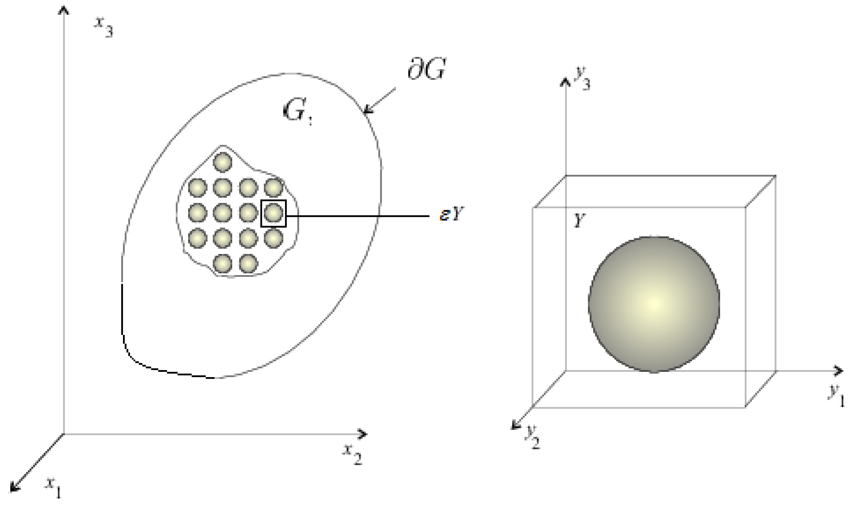
1.1. Asymptotic Expansions for the Elasticity Problem

The asymptotic expansions proposed in [2,3] for the problem without initial stresses can also be used for the analysis of the problem under consideration (for other homogenization techniques, see [4,5,6,7,8]). The expansions are the following: for displacements
u ε = u ( 0 ) ( x ) + k = 1 ε k u ( k ) ( x , y ) ,
for stresses
σ i j ε = k = 0 ε k σ i j ( k ) ( x , y ) .
We use the homogenization technique, which is based on the two-scale asymptotic approach [1,2,5]. In accordance with this approach, along with the initial variable x , we introduce the variable y = x / ε , which we formally consider independent. In the two-scale asymptotic approach, x is called a “slow” or “global” variable, and y is called a “fast” or “local” variable [1,3]. From a physical point of view, the first variable describes the behavior of the composite as a whole, globally, and second-locally.
Functions on the right-hand side (3), (4) are taken to be periodic in y with periodicity cell Y ( ε Y is the periodicity cell in the “slow” variables x and Y is the periodicity cell in the “fast” variables y ).
Denote by the average value over the periodicity cell Y in “fast” variables y .
Furthermore, for the functions u ( i ) ( x , y ) that are fast correctors to the homogenized solution u ( 0 ) ( x ) , we use the ansatz [1], Ch. 2
u ( i ) ( x , y ) = K i p q ( y ) u p ( 0 ) ( x ) x q , i = 1 , 2 , 3 ,
where K i p q ( y ) is periodic in y functions with the periodicity cell Y.
Using the two-scale expansion, we represent the differentiation operators as a sum of operators with respect to x and y [1,2]. For functions Z ( x , y ) of the variables x and y , as in (3), (4), this leads to the replacement of differentiation operators according to the following rule:
Z x i Z , i x + ε 1 Z , i y ( i = 1 , 2 , 3 ) ,
subscript “ , i x ” means / x i , and subscript “ , i y ” means / y i .
Following the general method developed in the homohenization theory [1,5], we have to derive the periodicity cell problem. By using the asymptotic expansion technique, the differentiation rule (6), and (5), we arrive at the following periodicity cell problem for a composite with initial stresses (see for details [9]):
( h i j m n ( x , y ) K m , n y p q + h i j p q ( x , y ) ) , j y = 0   in   Y , K p q ( y ) periodic   in   y with   the   periodic   cell   Y
and the following formula for the local stresses σ i j ( 0 ) in composite
σ i j ( 0 ) = ( h i j m n ( x , y ) K m , n y p q + h i j p q ( x , y ) ) u p , q x ( 0 ) ( x ) .
The function K p q ( y ) is defined by (7). The periodicity cell problem also refers to the “periodic cell problem” [1,5], “unit cell problem” [10] or “unit-cell problem” [11].
Averaging (8) over the periodicity cell Y, we obtain the homogenized constitutive equations
σ i j ( 0 ) = C i j k l ( σ ) u k , l x ( 0 ) ( x )
for the body with initial stresses. In (9),
C i j k l ( σ ) = h i j m n ( x , y ) K m , n y k l + h i j k l ( x , y )
are the homogenized elastic characteristics of the body with initial stresses.
The homogenized static equilibrium equation is the following:
( C i j k l ( σ ) u k , l x ( 0 ) ) , j x = f i .
From the boundary condition in (1) and expansion (3), we obtain the following boundary condition:
u ( 0 ) ( x ) = 0   on   G .
The problem (11), (12) is the homogenized static problem for a body with initial stresses. The homogenized dynamic problem has the form
( C i j k l ( σ ) u k , l x ( 0 ) ) , j x = ρ 2 u i ( 0 ) t 2 + f i .
Boundary conditions for Equation (13) have the form (12).
Equation (13) is valid under condition that the wavelength is significantly greater that the characteristic size ε of the periodic cell of the structure.
Unlike the homogenization problem for unstressed materials, now, the cell problem (7) depends on initial stresses. It leads to the dependence of the homogenized coefficients and the velocities of the elastic waves on the initial stresses.
Below, we will consider the orthotropic homogenized media. The velocities of the elastic waves in the direction of O x 1 -axis are: for longitudinal (compression) wave
c l ( σ ) = C 1111 ( σ ) ρ ,
for shear waves
c s h ( σ ) = C 2121 ( σ ) ρ ,
and
c s h ( σ ) = C 3131 ( σ ) ρ .
The velocities of the elastic waves in the other directions are obtained by the proper changing of the indices of the homogenized constants.
For the homogeneous bodies, the problems of elasticity theory as well as the velocities of the elastic waves also depend on the initial stresses [9,12]. The following questions appear:
-
These dependencies are the same or different for the homogeneous and the composite bodies;
-
If different, how large is the difference.

1.2. The Case of Small Initial Stresses

The initial stresses in the composite are limited by the strength limit of the components of the composite; thus, they do not exceed a few percent of the Young’s modulus. As we mention above, we suppose initial stresses are well within the elastic regime. Then, the coefficients h i j k l (2) can be represented as
h i j k l ( x , y ) = c i j k l ( y ) + S b i j k l ( x , y ) ,
m a x δ i k | σ j l * ( x , y ) | / c i j k l ( y ) S 0.01
for any x and y and i , j , k , l ; where b i j k l ( x , y ) are of the order of 1.
In (17), S is a small parameter. The meaning of S is the characteristic value of the initial stresses, usually, S 0.01.
To solve the cell problem (7) with the coefficients (17), we represent the solution in the form
K k l ( y ) = K 0 k l ( y ) + S K 1 k l ( y ) .
Substituting (18) into (7) and collecting the terms of the same order, we obtain
( c i j n m ( y ) K m , n y 0 k l + c i j k l ( y ) ) , j y = 0   in   Y , ( c i j n m ( y ) K m , n y 1 k l + b i j k l ( x , y ) + b i j k l ( x , y ) K m , n y 0 k l ( y ) ) , j y = 0   in   Y , K 0 k l ( y ) , K 1 k l ( y ) periodic   in   y   with   the   periodicity   cell   Y .
We note that
K 0 k l ( x ) = N k l ( x ) ,
where N k l is the solution to the cell problem for the body without initial stresses [1,2]:
( c i j n m ( y ) N m , n y k l + c i j k l ( y ) ) , j y = 0   in   Y , N k l ( y ) periodic   in   y   with   the   periodicity   cell   Y .
Formula (10) may be transformed into the following form [13]
C i j k l ( σ ) = C i j k l ( 0 ) + S σ q n * ( x , y ) δ i k + S C i j k l 1 ( σ ) ,
where C i j k l ( 0 ) represents the homogenized elastic constants of the body without initial stresses and
C i j k l 1 ( σ ) = σ q n * ( x , y ) N p , n y k l ( y ) N p , q y i j ( y ) ,
where N k l ( x ) is the solution to the cell problem (20).
The sum of the first and the second terms in the right-hand part of Equation (21) corresponds to the “intermediate” homogenization, when first, the homogenized constants are calculated for the composite material without initial stresses, and then, the composite is treated as a homogeneous material subjected to initial stresses. The first and the second terms in the right-hand part of Equation (21) represent the elastic constant and average value of the initial stresses. The last term in (21) arises as a result of the homogenization of the composite material with the initial stresses. For homogeneous materials, N k l ( x ) = 0 and the last term in (21) is zero. For inhomogeneous (composite) materials, the last term in (21) is, generally speaking, not zero.
Formula (22) involves the partial derivatives of N k l ( y ) . Write the Formula (22) in the terms of the strain tensor 2 e i j k l = N i , j k l + N j , i k l and the rotation tensor 2 ω i j = N i , j k l N j , i k l . We have
C i j k l 1 ( σ ) = σ q n * ( x , y ) ( e p n k l ( y ) + ω p n k l ( y ) ) ( e p q i j ( y ) + ω p q i j ( y ) ) .
Formula (23) is suitable for numerical computations with the commercial software. If the initial stresses σ q n * are determined from solutions to the elasticity theory problem (1), (2), then [1]
σ i j ( 0 ) = ( c i j m n ( x , y ) N m , n y p q + c i j p q ( x , y ) ) u p , q x ( 0 ) ( x ) = ( c i j m n ( x , y ) e m n p q + c i j p q ( x , y ) ) u p , q x ( 0 ) ( x ) .

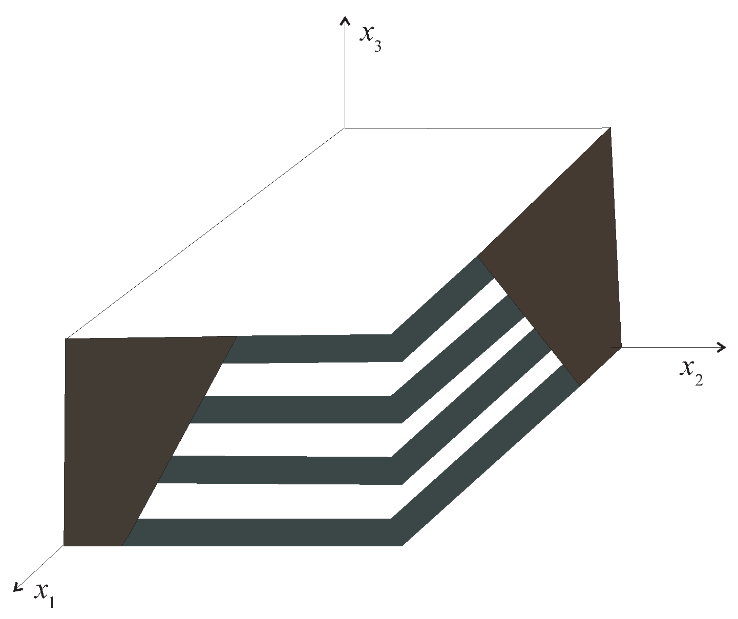
2. Laminated Materials with Initial Stresses

In this section, we apply the method developed above to the laminated materials with initial stresses. Let the layers be parallel to the plane O x 1 x 2 , as shown in Figure 2. In this case, all the functions of the variable y = ( y 1 , y 2 , y 3 ) become the functions of the variable y 3 . In particular, the periodicity cell problem (7) takes the form
( h i 3 k 3 ( x , y 3 ) K k p q + h i 3 p q ( x , y 3 ) ) = 0   in   [ 0 , 1 ] , K p q ( y 3 ) periodic   in y 3 with   period   [ 0 , 1 ] .
In (24), prime means the derivative with respect to y 3 .
Problem (24) is a periodic problem for a system of ordinary differential equations. It may be solved in explicit form.
From the equation in (24), it follows that h i 3 k 3 ( x , y 3 ) K k p q + h i 3 p q ( x , y 3 ) = C i p q . Thus,
K i p q = ( h i 3 k 3 ( x , y 3 ) ) 1 h i 3 p q ( x , y 3 ) + ( h i 3 k 3 ( x , y 3 ) ) 1 ( C i p q ) ,
where { C k p q } are constants, and symbol ( . . . ) 1 means the matrix inversion.
The constants C k p q in (25) are determinable from the periodicity condition for K p q , which may be written in the form
K p q = 0 .
For the laminated materials, the average value is computed as
Z = 0 1 Z ( y 3 ) d y 3 = I = 1 m Z I λ I ,
where λ I is the volume fraction of the I-th material, and m is the total number of materials.
The period is assumed to be 1, which does not restrict the generality of the computations.
Substituting (25) into (26), we obtain
( h i 3 k 3 ( x , y 3 ) ) 1 h i 3 p q ( x , y 3 ) = ( h i 3 k 3 ( x , y 3 ) ) 1 C i p q .
By solving this system of linear algebraic Equation (28) with respect to C k p q , we obtain
C k p q = ( h i 3 k 3 ( x , y 3 ) ) 1 1 ( h j 3 k 3 ( x , y 3 ) ) 1 h j 3 p q ( x , y 3 ) .
Substituting (29) into (25), we have
K k p q = ( h i 3 k 3 ( x , y 3 ) ) 1 h i 3 p q ( x , y 3 ) + ( h i 3 k 3 ( x , y 3 ) ) 1 ( h i 3 k 3 ( x , y 3 ) ) 1 1 ( h j 3 k 3 ( x , y 3 ) ) 1 h j 3 p q ( x , y 3 ) .
Since the initial stresses are relatively small, we have a matrix with prevailing diagonal terms. It is easy to show that this matrix is well conditioned, so its inversion is a well-posed problem.
In the case under consideration, Formula (10) for the homogenized characteristics takes the form
C i j k l ( σ ) = h i j p 3 ( x , y 3 ) K p k l + h i j k l ( x , y 3 ) .
Substituting (30) into (31), we obtain
C i j k l ( σ ) = h i j k l ( x , y 3 ) h i j m 3 ( x , y 3 ) ( h m 3 n 3 ( x , y 3 ) ) 1 h n 3 k l ( x , y 3 ) + h i j m 3 ( x , y 3 ) ( h m 3 n 3 ( x , y 3 ) ) 1 ( h n 3 p 3 ( x , y 3 ) ) 1 1 × ( h p 3 q 3 ( x , y 3 ) ) 1 h q 3 k l ( x , y 3 ) .
Consider the material formed of the layers of homogeneous orthotropic materials. In this case
h i 3 k 3 ( x , y 3 ) = c i 3 k 3 ( y ) + σ 33 * ( x , y 3 ) δ i k .
Note that h i 3 k 3 = 0   if   i k ( c i 3 k 3 = 0   if   i k for orthotropic materials [14]), i.e., h i 3 k 3 is a diagonal matrix, and its inverse matrix is
( h m 3 m 3 ( x , y 3 ) ) 1 = 1 h m 3 m 3 ( x , y 3 ) , ( h m 3 k 3 ( x , y 3 ) ) 1 = 0   if   m k ,
By virtue of (33), Equation (32) takes the form
C i j k l ( σ ) = h i j k l h i j m 3 h n 3 k l h m 3 n 3 + h i j m 3 h m 3 n 3 h q 3 k l h p 3 q 3 1 h n 3 p 3 .
By using the definition of the constants h i j k l (2) and equality (33), we write the homogenized constants (34), which depend on σ i j * , in the form
C 3333 ( σ ) = 1 1 c 3333 + σ 33 * ; C 3322 ( σ ) = c 3322 c 3333 + σ 33 * 1 c 3333 + σ 33 * ;
C 1313 ( σ ) = C 2323 ( σ ) = 1 1 c 2323 + σ 33 * ; C 3232 ( σ ) = c 3232 + σ 22 * c 2323 2 c 3333 + σ 33 * + c 2323 c 3333 + σ 33 * 2 1 c 3333 + σ 33 * ;
C 1111 ( σ ) = c 1111 + σ 11 * c 1133 2 c 3333 + σ 33 * + c 1133 c 3333 + σ 33 * 2 1 c 3333 + σ 33 * ;
C 1122 ( σ ) = c 1122 c 1133 c 2233 c 3333 + σ 33 * + c 3322 c 3333 + σ 33 * c 3322 c 3333 + σ 33 * 1 c 3333 + σ 33 * .
In (35), c i j k l = c i j k l ( y 3 ) and σ i j * = σ i j * ( x , y 3 ) .
The first formula in (35) coincides with the corresponding formula from [12]. Nevertheless, most of the formulas in (35) do not coincide with the formulas from [12].

2.1. One Special Case

Consider the initial stresses of the form
σ i i * = σ i i * ( y 3 )
with condition
σ i j * = σ i j = c o n s t .
The stresses (36) satisfy Equation (1) with f = f ( y 3 ) . Such a kind of stress-strain state arises in a laminated rock massif, for example, under the action of the force of gravity.
Substituting (36) into (35), we obtain C i j k l ( σ ) as a function of macroscopis stress σ i j .
Let us consider a body formed by layers of isotropic materials. In this case, the local elastic constants have the form
c i j k l = E ν ( 1 + ν ) ( 1 2 ν ) δ i j δ k l + E 1 + ν δ i k δ i k ,
where E = E ( y 3 ) is the local Young’s modulus and ν = ν ( y 3 ) is the local Poisson’s coefficient.
Substituting (36) and (38) into (35), we obtain
C 3333 ( σ ) = 1 ( 1 + ν ) ( 1 2 ν ) ( 1 ν ) E + σ 33 ( 1 + ν ) ( 1 2 ν ) ;
C 3232 ( σ ) = E 1 + ν E 2 ( 1 + ν ) E + ( 1 + ν ) 2 σ 33 + E E + ( 1 + ν ) σ 33 2 1 + ν E + ( 1 + ν ) σ 33 + σ 22 ;
C 1313 ( σ ) = C 2323 ( σ ) = 1 1 + ν E + σ 33 ( 1 + ν ) ;
C 1111 ( σ ) = ( 1 ν ) E ( 1 + ν ) ( 1 2 ν ) E 2 ν 2 ( 1 ν 2 ) ( 1 2 ν ) E + ( 1 + ν ) 2 ( 1 2 ν ) 2 σ 33 + E ν ( 1 ν ) E + ( 1 + ν ) ( 1 2 ν ) σ 33 2 ( 1 + ν ) ( 1 2 ν ) E + ( 1 ν ) σ 33 + σ 11 ;
C 1122 ( σ ) = E ν ( 1 + ν ) ( 1 2 ν ) E 2 ν 2 ( 1 ν 2 ) ( 1 2 ν ) E + ( 1 + ν ) 2 ( 1 2 ν ) 2 σ 33 + E ν ( 1 ν ) E + ( 1 + ν ) ( 1 2 ν ) σ 33 ( 1 + ν ) ( 1 2 ν ) E + ( 1 ν ) σ 33 .
As can be seen from Formula (39), the dependence of C i j k l ( σ ) on σ i j is rather complicated even in the considered simplest case of laminated material.
Figure 3 shows the graph of the function
z ( σ 33 ) = C 3333 ( σ 33 ) C 3333 + σ 33
in dependence on σ 33 for the case when all overall stresses, except for σ 33 , are zero. The function z ( σ 33 ) is computed for a two-layer composite. The Young’s moduli of the layers are E = 1 MPa and E = 2 MPa, and Poisson’s ratio is ν = 1 / 3 for both the layers.
Formula (40) gives the ratio of the velocities of elastic waves calculated by Formula (39) and by the “intermediate” homogenization. The value y ( 1.5 ) = 0 means that the velocities of elastic waves predicted by Formula (39) decrease faster than the one predicted by the “intermediate” homogenization.

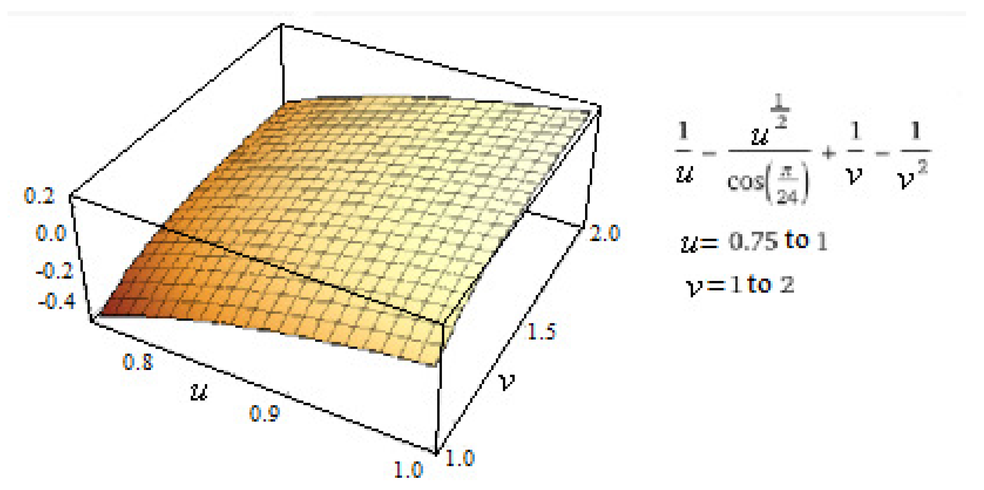
2.2. Small Initial Stresses

As noted, the initial stresses are small. By using this remark, one can expand Formula (39) in series with respect to the small dimensionaless parameter σ 33 / E . Keeping only the linear terms, we obtain:
C 3333 ( σ ) = C 3333 ( 0 ) + σ 33 + ( 1 + ν ) 2 ( 1 2 ν ) 2 ( 1 ν ) 2 E 2 ( 1 + ν ) ( 1 2 ν ) ( 1 ν ) E 2 1 σ 33 ;
C 3322 ( σ ) = C 3322 ( 0 ) + ν ( 1 + ν ) ( 1 2 ν ) ( 1 ν 2 ) E ( 1 + ν ) ( 1 2 ν ) ( 1 ν ) E + ν 1 + ν ( 1 + ν ) 2 ( 1 2 ν ) 2 ( 1 ν ) 2 E 2 ( 1 + ν ) ( 1 2 ν ) ( 1 ν ) E 2 σ 33 ;
C 2323 ( σ ) = C 2323 ( 0 ) + σ 33 + ( 1 + ν ) 2 E 2 1 + ν E 2 1 σ 33 ;
C 3232 ( σ ) = C 3232 ( 0 ) + σ 22 + ( 1 + ν ) 2 E 2 1 + ν E 2 1 σ 33 ;
C 1111 ( σ ) = C 1111 ( 0 ) + σ 11 + [ ν 2 ( 1 ν ) 2 2 ν ( 1 + ν ) ( 1 2 ν ) ( 1 ν ) 2 E ν 1 ν ( 1 + ν ) ( 1 2 ν ) ( 1 ν ) E + ν 1 ν ( 1 + ν ) 2 ( 1 2 ν ) 2 ( 1 v ) 2 E 2 ( 1 + ν ) ( 1 2 ν ) ( 1 ν ) E 2 ] σ 33 ;
C 1122 ( σ ) = C 1122 ( 0 ) + [ ν 2 ( 1 ν ) 2 2 ν ( 1 + ν ) ( 1 2 ν ) ( 1 ν ) 2 E ν 1 ν ( 1 + ν ) ( 1 2 ν ) ( 1 ν ) E + ν 1 ν ( 1 + ν ) 2 ( 1 2 ν ) 2 ( 1 ν ) 2 E 2 ( 1 + ν ) ( 1 2 ν ) ( 1 ν ) E 2 ] σ 33 .
Formula (41) has the form
C i j k l ( σ ) = [ C i j k l ( 0 ) + σ j l δ i k ] + C i j k l 1 σ 33 .
The bracketed expression in (42) corresponds to the “intermediate” homogenization. The last term in (42) arises as a result of the homogenization of the original composite material with the initial stresses.
In the case ν = c o n s t , Formula (42) is significantly simplified and takes the form
C 3333 ( σ ) = C 3333 ( 0 ) + ( 1 + L ) σ 33 , C 3322 ( σ ) = C 3322 ( 0 ) + ν 1 ν L σ 33 , C 2323 ( σ ) = C 2323 ( 0 ) + ( 1 + L ) σ 33 , C 3232 ( σ ) = C 2323 ( 0 ) + σ 22 + L σ 33 , C 1111 ( σ ) = C 1111 ( 0 ) + σ 11 + ν 2 1 ν 2 L σ 33 , C 1122 ( σ ) = C 1122 ( 0 ) + ν 2 1 ν 2 L σ 33 , C 1212 ( σ ) = C 1212 ( 0 ) ,
where
L = 1 E 2 / 1 E 2 1 .
It is seen that all coefficients C i j k l 1 in (43) depend on the only parameter L (44). By using the method of convex combinations [15,16], we conclude that the pair ( 1 / E 2 , 1 / E ) may take any values ( X , Y ) satisfying the condition X > Y 2 . Then, L can take an arbitrary positive value. As a result, for σ 33 > 0
C i j k l ( σ ) C i j k l + σ j l δ i k ,
and the difference between C i j k l ( σ ) and C i j k l + σ j l δ i k can take an arbitrary positive value.
Example. Consider a layered composite made of materials with E 1 = 1 × 10 10 , E 2 = 0.01 × 10 10 , and ν = 0.3 for both λ 1 = 0.9 and λ 2 = 0.1 . For this composite, L 10 2 and C 3333 = 0.136 × 10 10 ( C 3333 is computaed in accordance with the homogenization theory). Substituting these values to the first formula in (43), we arrive at the following:
C 3333 ( σ ) = C 3333 ( 0 ) + ( 1 + L ) σ 33 = 0.136 × 10 10 + σ 33 + 10 σ 33 .
In this formula
-
0.136 × 10 10 —the homogenized elastic constant of the composite without initial stresses;
-
σ 33 —the term corresponding to the “intermediate” homogenization;
-
10 σ 33 —the term C 3333 1 σ 33 .
The value of the last term significantly exceeds the term corresponding to the “intermediate” homogenization.

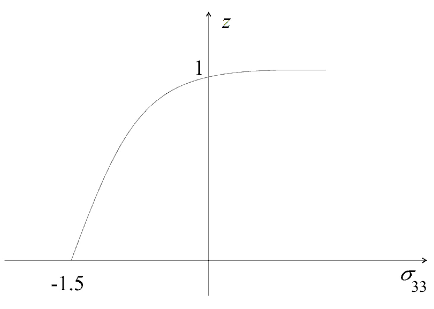
2.3. The Homogenized Velocity of the Elastic Waves

Using Formula (43), write the formulas for the velocities of the elastic waves: the velocity of the longitudinal (compression) wave in the direction of the O x 1 -axis
c l ( σ ) = C 1111 ( 0 ) + σ 11 + ν 2 1 ν 2 L σ 33 ρ ,
the velocity of the shear waves
c s h ( σ ) = C 2121 ( 0 ) ρ ,
and
c s h ( σ ) = C 2323 ( 0 ) + ( 1 + L ) σ 33 ρ .

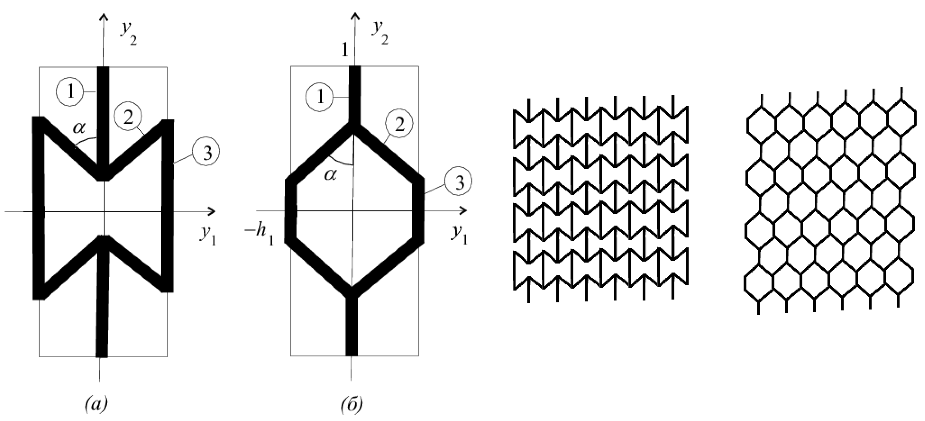
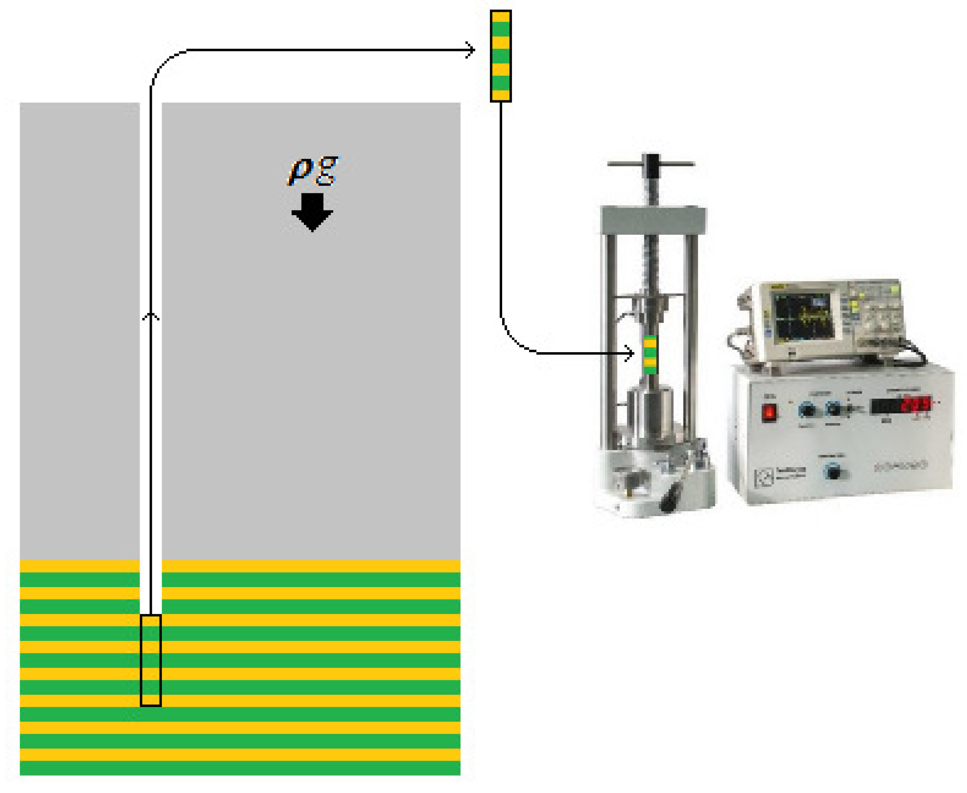
3. The Non-Trivial Dependence of Speed of Elastic Waves on the Initial Stress in the “Inverted Honeycomb” Frame Structure

The previous section provides us with an example of the quantitative defference of the dependence of elastic waves velocity on initial stress in the homogeneous and inhomogeneous media. In this section, we present an example of the qualitative difference of the dependence of elastic waves velocity on initial stress in the homogeneous and inhomogeneous media. For this reason, we conside special high-porous materials “honeycomb” framework materials. The “honeycomb” materials are widely used in paractice. The geometry of the honeycomb essentially influences the homogenized properties of the “honeycomb” material. The “honeycomb” materials are widely used as models of the foams and high-porous materials, see, e.g., [17,18]. The analyzed frame composite can be used for the modeling of porous media.
If the periodicity cell of a composite is formed by beams and/or plates (lattices, openwork ceilings, etc.), then the methods of the beam and/or plate theories can be applied to solve the cell problem. In some cases, the problem may be solved in explicit form.
Let us consider a periodic structure formed by rods. This is a special case of frame structures. In this case, Equations (17) and (7) can be replaced [19] by the cell problem for the corresponding cell structure formed from a system of beams and/or plates (see also [15,20]).
The velocity c 22 h ( σ ) of the longitudinal elastic waves along the axis O x 2 in the homogeneous elastic material with initial stress σ 22 is
c 22 h ( σ ) = c 2222 h + σ 22 ρ h ,
where c 2222 h is the elastic constant, and ρ h is the density of the homogeneous material.
The dependence of the velocity of the longitudinal long elastic waves for the homogeneous material is monotone: for σ 22 < 0
c 22 h ( σ ) < c 22 h ( 0 )
and for σ 22 > 0
c 22 h ( σ ) > c 22 h ( 0 ) .
The velocity of the longitudinal long elastic waves along the axis O x 2 in the elastic composite material is equal to
c 22 ( σ ) = C 2222 ( σ ) ρ ,
where C 2222 ( σ ) is the homogenized elastic constant, and ρ is the homogenized density of the composite material.
This section presents an example demonstrating that the dependence of the velocity of the elastic waves on the initial stress may be not monotonic for composite materials. Such a phenomenon never occurs in homogeneous bodies.
Consider the composite whose periodicity cell is shown in Figure 4a. It is the so-called inverted honeycomb. The inverted honeycomb was introduced in [19] to construct a composite with a negative Poisson’s ratio. It was modified in [21] to construct an isotropic three-dimensional structure with Poisson’s ratio equal to 1 . Following [19], the composite with a negative Poisson’s ratio was investigated by numerous authors, see, e.g., [22,23,24,25,26,27,28,29,30,31,32] (the list is not completed; see current references in [33,34,35,36,37,38]).
When applying an overall compressive stress
σ i j = σ 22 δ i 2 δ j 2 ,
in the elements of the standard honeycomb cell, see Figure 4b, only compressive stresses arise. In the elements of the inverted honeycomb cell, see Figure 4a, both compressive and tensile stresses arise.
Let us calculate C i j k l ( σ ) in the case when the overall stresses have the form σ 22 = σ < 0 (the coordinate axes are displayed in Figure 4) and σ i j = 0 for i j 22 . Let us calculate C 2222 ( σ ) . The other homogenized constants are calculated in the same way.
Compute the local initial stresses in the elements of the structure. We assume that the elements are rods and act only in the tension–compression mode (we can neglect the bending stresses in the rods). Denote by E 1 , E 2 , E 3 the axial stiffness of rods and by h 1 , h 2 , h 3 the thickness of rods. The element numbering is shown in Figure 4. The local stresses in periodicity cell elements σ 1 , σ 2 , σ 3 are the following:
σ 1 * = σ , h 3 σ 3 * = h 1 σ 1 , h 2 σ 2 * c o s α = h 1 σ 1 * .
The solution to (51) is
σ 1 * = σ , σ 3 * = h 1 h 3 σ , σ 2 * = h 1 h 2 1 c o s ( α ) σ .
In order to calculate C 2222 ( σ ) , one has to solve the cell problem for the structure shown in Figure 4, replacing the Young’s moduli E p to E p + σ p * ( p = 1 , 2 , 3 ), where σ p * are the initial stresses given by (52). Here, p is the number of the rod in the cell structure; see Figure 4. Denoting by e 1 , e 2 , e 3 the strains in the pre-stressed rods, we arrive at the equations (the total strain of the cell along the O y 2 axis is assumed to be 1)
( E 1 + σ 1 * ) e 1 h 1 = ( E 3 + σ 3 * ) e 3 h 3 , ( E 2 + σ 2 * ) e 2 h 2 c o s α = ( E 1 + σ 1 * ) e 1 h 1 , e 1 e 2 c o s α + e 3 = 1 .
From (53), we have
e 3 = E 1 + σ 1 * E 3 + σ 3 * h 1 h 3 e 1 , e 2 = E 1 + σ 1 * E 2 + σ 2 * h 1 h 2 1 c o s ( α ) e 1 , e 1 e 2 c o s α + e 3 = 1 .
The last equation in (54) leads to
[ 1 + E 1 + σ 1 * E 2 + σ 2 * h 1 h 2 + E 1 + σ 1 * E 3 + σ 3 * h 1 h 3 ] e 1 = 1 .
The effective elastic constant is
C 2222 ( σ ) = h 1 E 1 e 1 ,
where e 1 is determined from (55).
Substituting σ 1 * , σ 2 * , σ 3 * according to (52) into (55), we obtain from (56) that
C 2222 ( σ ) = h 1 E 1 · 1 1 + E 1 + σ 1 * E 2 + σ 2 * h 1 h 2 + E 1 + σ 1 * E 3 + σ 3 * h 1 h 3 .
Formula (57) is valid for any (arbitrary) stress σ 22 . Now, consider Formula (57) for small initial stresses, namely, for | σ 22 | E 1 . Let us rewrite (57) as follows:
C 2222 ( σ ) = h 1 E 1 · 1 1 + 1 + σ E 1 E 2 E 1 h 1 h 2 1 c o s ( α ) σ E 1 h 1 h 2 + 1 + σ E 1 E 3 E 1 + h 1 h 3 σ E 1 h 1 h 3 .
and consider the denominator in (58)
1 + 1 + s e 2 h 1 h 2 1 c o s ( α ) s h 1 h 2 + 1 + s e 3 + h 1 h 3 s h 1 h 3 .
Denoted: s = σ E 1 , r 2 = E 2 E 1 , r 3 = E 3 E 1 . Using expansion 1 r i + Θ 1 r i Θ r i 2 for small Θ , extract the linear term in σ in (59)
1 + 1 r 2 + σ r 2 1 r 2 2 h 1 h 2 1 c o s α s h 1 h 2 + 1 r 3 + r 3 1 r 3 2 h 1 h 3 s h 1 h 3 = 1 + 1 r 2 h 1 h 2 + 1 r 3 h 1 h 3 + σ r 2 h 1 h 2 1 r 2 2 h 1 h 2 1 c o s α s h 1 h 2 + σ r 3 h 1 h 3 1 r 3 2 h 1 h 3 s h 1 h 3 = 1 + 1 r 2 h 1 h 2 + 1 r 3 h 1 h 3 + 1 r 2 h 1 h 2 1 r 2 2 h 1 h 2 2 1 c o s α + 1 r 3 h 1 h 3 1 r 3 2 h 1 h 3 2 .
The sum in the first square brackets in the right-hand part of Equation (60) is the effective elastic constants C 2222 ( 0 ) of the frame structure without initial stresses. The sum in the second square brackets in the right-hand part of Equation (60) accounts for the initial stresses. In (60), we put h 1 = 1 . It does not restrict the generality of the consideration but simplifies the formulas below. For h 1 = 1 , the sum in the second square brackets in the right-hand part of Equation (60) can be written as follows:
1 r 2 h 2 1 r 2 2 h 2 2 c o s α + 1 r 3 h 3 1 r 3 2 h 3 2 .
Formula (61) has the form
1 u 1 u 2 c o s α + 1 v 1 v 2 ,
where u = r 2 h 2 and v = r 3 h 3 .
The plot of the function (62) is displayed in Figure 5 for α = π / 12 , 0.5 u 1.5 , 1.1 v 3.6 . It is seen that the function (62) can take both positive and negative values. Thus, the effective elastic constant C 2222 ( σ ) of the frame composite with initial stresses may be both less and greater than the effective elastic constant C 2222 ( 0 ) of the frame composite without initial stresses.
In particular, if σ 22 = σ < 0 , it is possible to satisfy the inequality
c 22 ( σ ) < c 22 ( 0 )
as well as the inequality
c 22 ( σ ) > c 22 ( 0 ) ,
where
c 22 ( 0 ) = C 2222 ( 0 ) ρ
is the velocity of the longitudinal elastic waves along the axis O x 2 in the composite without initial stresses. Thus, in the cellular materials, the compressed stress may both increase and decrease the velocity of the elastic waves.
For the standard honeycomb cell, Figure 4b, the sign of the axial stress in the structural elements coincides with the sign of the overall stress σ 22 . The standard honeycomb cell structure qualitatively demonstrates the behavior similar to the behavior of a homogeneous body.

4. The Problem of “Intermediate” Homogenization

The “intermediate” homogenization has been mentioned several times above. Let us discuss this concept in more detail. The “intermediate” homogenization method arises from the phenomenological approach to inhomogeneous bodies. If one investigates the properties of the bowels of a rock massif, one usually drills a well and extracts a core sample from the massif (Figure 6); see [39,40,41,42] for detail. When extracting the core sample from the massif, one determines the overall characteristics of the sample. The overall characteristics determined in such a way are exactly the homogenized elastic constants C i j k l ( 0 ) . When the homogenized elastic constants C i j k l ( 0 ) are determined, one solves the problem (11), (12) to determine the stresses σ i j in the rock massif. Then, C i j k l ( 0 ) and σ i j are used for subsequent computations in accordance with the classical theory of the homogeneous elastic bodies with initial stresses [12,43].
Since the scheme presented in Figure 6 is widely used, we would like to discuss the potential problems related to this scheme as applied to the computation of stong inhomogeneous materials with initial stresses.
The “intermediate” homogenization, generally, leads to a wrong result. Let us start with the mathematical aspects of the problem. From the mathematical point of view, we deal with the homogenization problem for the sum of the operators
L ε u = [ c i j k l ( x / " ) u k , l ) ] , j
and
M ε u = ( δ i k σ j l * ( x , x / " ) u k , l ) , j .
The problem of homogenization [44,45] for a sum of operators of the same order (this is our case) is not solved until now. The suggestion, which seems reasonable from the common point of view, is to follow the theory developed for homogeneous materials and calculate the homogenized constant as follows (compare with (2))
C i j k l ( σ ) = C i j k l ( 0 ) + δ i k σ j l * ( x , y ) ,
or, which is the same, write the homogenized problem in the form
L ( 0 ) u + M u = u ,
where
L ( 0 ) u = [ C i j k l ( 0 ) u k , l ) ] , j , M u = ( δ i k σ j l * u k , l ) , j .
Here, C i j k l ( 0 ) represents the homogenized constants of the body without initial stresses. Problem (65) is equivalent to the problem of minimization of the functional [43]
J 0 ( u ) + I 0 ( u ) ( f , u ) L 2 ,
where
J 0 ( u ) = 1 2 G C i j k l ( 0 ) e i j e k l d x , I 0 ( u ) = 1 2 G σ j l * e i j e i l d x .
In accordance with the homogenization theory [1] σ i j * = σ i j , where σ i j are the homogenized stresses computed from the problem (11), (12).
As was mentioned above, determining the effective elastic constant C i j k l ( σ ) is equivalent to calculating the G-limit of the sum L ε + M ε ; see (63), (64). In doing so, it is necessary to express the G-limit through limits (of any kind) of operator L ε (63) with the coefficients C i j k l ( x / ε ) and operator M ε (64) with the coefficients σ i j * ( x , x / ε ) . The equivalent problem is the computation of the limit l i m ε 0 ( I ε + J ε ) * ( v * ) (the asterisk means the dual functional), where I ε and J ε are potentials of the operators L ε and M ε , (63) and (64). Little is known about the mentioned problems. However, it is known [45] that no rule like “the limit of the sum is equal to the sum of the limits” (or another similar simple rule) exists for the discussed problems.
This is the reason for the appearance of the difference between the dependence of the elastic properties of inhomogeneous solids and the same dependence for homogeneous solids.
From the mechanical viewpoint, the inapplicability of the “intermediate” homogenization is the result of the occurrence of a general stress–strain state at the microlevel when the uniform homogenized stresses are applied at the macrolevel. There are other methods of micromechanics and simulations which may be potentially applied to the analysis of the pre-stressed composites, see, e.g., [46,47,48].

5. Conclusions

In the paper, the general approach to the homogenization of composites with initial stresses is presented.
We discuss an interesting question from the point of view of mechanics—how an inhomogeneous structure changes the dependence of the wave velocity on the initial stresses in comparison with the corresponding dependence for a homogeneous material. The question of the dependence of the velocity of elastic waves on the initial stresses is traditional for the theory of elasticity. The main result of our article can be formulated as follows: the microstructure can change the dependence of the wave velocity in the composite on the initial stresses both qualitatively and quantitatively. This result seems to us to be new, interesting, and confirmed by the above results.
In order not to overload the article with mathematical calculations, we considered several particular problems that are directly related to practice: the velocity of elastic waves in layered media with initial stresses and frame-like composites with initial stresses.
The analyzed frame composite can be used for the modeling of porous media.
Explicit formulas are obtained for the homogenized coefficients of the laminated and honeycomb composites. We investigated the dependencies of the homogenized coefficients and velocity of the elastic waves on the macroscopic initial stresses. It is found that the dependencies for composite bodies differ from the dependencies for homogeneous bodies. For the laminated bodies, the difference from homogeneous bodies is quantitative; see Section 2. The initial tension increases the velocity of elastic waves in both cases, but the quantitative effect of the increase can vary greatly. For frame composites modeling porous bodies, the initial tension can increase or decrease the velocity of elastic waves (the initial tension decreases the velocity of elastic waves in the porous body with inverted honeycomb periodicity cells). The decrease of the velocity of elastic waves is impossible in homogeneous media. Note that layered and porous structures with initial stresses are widely encountered in practice [39,40,41,42].
In Section 4, we pay the attention to the methodology of measuring and calculating core properties. For composite materials, it is a non-trivial problem. The solution to the problem, evident from the common point of view, is the “intermediate” homogenization. It is the case when the “evident” method is not valid.
The homogenization of the elasticity theory problem with initial stresses may be completed by obtaining special cases in explicit form. There is no explicit, or even simple, solution to the problem in the general case. In the general case, as follows from Section 1, the homogenization problem may be solved for specific material numerically by using the appropriate mathematical methods. Note that the commercial numerical sofware (ANSYS and similar FEM software) is not adopted for the solution of such kinds of problems.
The evident way to verify the results obtained in this manuscript is the numerical solution of the dynamical elasticity problem for a laminated media with initial stresses. The authors do not have information about such types of published papers. So, the authors cannot conclude for sure whether such a problem may be solved with commercial software. If it can be completed, the solution will require a separate paper.

Author Contributions

Conceptualization, A.G.K.; methodology, A.G.K., I.V.A. and S.I.R.; investigation, A.G.K., S.I.R. and A.G.K.; writing—original draft preparation, A.G.K.; software, S.I.R.; writing—review and editing, I.V.A. and A.G.K.; formal analysis, A.G.K., I.V.A. and S.I.R. All authors have read and agreed to the published version of the manuscript.

Funding

This research received no external funding.

Institutional Review Board Statement

Not applicable.

Informed Consent Statement

Not applicable.

Data Availability Statement

Data are contained within the article.

Conflicts of Interest

The authors declare no conflict of interest.

References

  1. Bakhvalov, N.S.; Panasenko, G.P. Homogenisation: Averaging Processes in Periodic Media; Kluwer: Dordrecht, The Netherlands, 1989. [Google Scholar]
  2. Sanchez-Palencia, E. Non-Homogeneous Media and Vibration Theory; Springer: Berlin/Heidelberg, Germany, 1980. [Google Scholar]
  3. Sanchez-Palencia, E. Equations aux deivees partielles. Solutions periodiques par repport aux variables d’espace et application. Comp. Rend. Acad. Sci. Paris Ser. A 1970, 271, 1129–1132. [Google Scholar]
  4. Alaire, G. Homogenization and two–scale convergence. SIAM J. Math. Anal. 1992, 23, 1482–1518. [Google Scholar] [CrossRef]
  5. Bensoussan, A.; Lions, J.-L.; Papanicolaou, G. Asymptotic Analysis for Periodic Structures; North–Holland Publ.: Amsterdam, The Netherlands, 1978. [Google Scholar]
  6. Jikov, V.V.; Kozlov, S.M.; Oleinik, O.A. Homogenization of Differential Operators and Integral Functionals; Springer: Berlin/Heidelberg, Germany, 1994. [Google Scholar]
  7. Kolpakov, A.G. Averaging of some systems of ordinary differential equations. Math. USSR-Sb. 1982, 119, 534–547. [Google Scholar] [CrossRef]
  8. Spagnolo, S. Sul limite delle soluzioni di problemi di Cauchy relativi all’equazione dell calore. Annali della Scuola Normale Superiore di Pisa 1967, 21, 657–699. [Google Scholar]
  9. Kolpakov, A.G. Stressed Composite Structures: Homogenized Models for Thin–Walled Nonhomogeneous Structures with Initial Stresses; Springer: Berlin/Heidelberg, Germany, 2004. [Google Scholar]
  10. Xing, Y.F.; Gao, Y.H.; Chen, L.; Li, M. Solution methods for two key problems in multiscale asymptotic expansion method. Compos. Struct. 2017, 160, 854–866. [Google Scholar] [CrossRef]
  11. Fergoug, M.; Parret-Freaud, A.; Feld, N.; March, B.; Forest, S. A general boundary layer corrector for the asymptotic homogenization of elastic linear composite structures. Compos. Struct. 2022, 285, 115091. [Google Scholar] [CrossRef]
  12. Guz, A.N. Elastic Waves in Bodies with Initial Stresses. In 2 Volumes. Vol. 1. General Questions. Vol. 2. Regularities of Wave Propagation; Naukova Dumka: Kiev, Ukraine, 1986. (In Russian) [Google Scholar]
  13. Kolpakov, A.G. Effect of influation of initial stresses on the homogenized characteristics of composite. Mech. Mater. 2005, 37, 840–854. [Google Scholar] [CrossRef]
  14. Lekhnitskii, S.G. Theory of Elasticity of an Anisotropic Elastic Body; Holden-Day: San Francisco, CA, USA, 1963. [Google Scholar]
  15. Kalamkarov, A.L.; Kolpakov, A.G. Analysis, Design and Optimization of Composite Structures; John Wiley & Sons: Chichester, UK, 1997. [Google Scholar]
  16. Kolpakov, A.A.; Kolpakov, A.G. Capacity and Transport in Contrast Composite Structures: Asymptotic Analysis and Applications; CRC Press: Boca Raton, FL, USA, 2010. [Google Scholar]
  17. Gibson, L.J.; Ashby, M.F. Cellular Solids; Cambridge Univ. Press: Cambridge, UK, 1987. [Google Scholar]
  18. Bahrant, J.; Ashby, M.F.; Fleck, N.A. Cellular Metals and Metal Foaming Technology; Verlag MIT Publ.: Bremen, Germany, 2001. [Google Scholar]
  19. Kolpakov, A.G. Determination of the average characteristics of elastic frameworks. J. Appl. Math. Mech. 1985, 49, 739–745. [Google Scholar] [CrossRef]
  20. Andrianov, I.; Awrejcewicz, J.; Manevitch, L.I. Asymptotical Mechanics of Thin–Walled Structures; Springer: Berlin/Heidelberg, Germany, 2004. [Google Scholar]
  21. Almgren, R.F. An isotropic three–dimensional structure with Poisson’s ratio = −1. J. Elast. 1985, 15, 427–430. [Google Scholar]
  22. Friis, E.A.; Lakes, R.S.; Park, J.B. Negative Poisson’s ratio polymeric and metalic foams. J. Mater. Sci. 1988, 23, 4406–4414. [Google Scholar] [CrossRef]
  23. Evans, K.E. Tensile network microstructures exhibiting negative Poisson’s ratios. Phys. D Appl. Phys. 1989, 22, 1870–1876. [Google Scholar] [CrossRef]
  24. Alderson, K.L.; Evans, K.E. The fabrication of microporous polyethylene having a negative Poisson’s ratio. Polymer 1992, 33, 4435–4438. [Google Scholar] [CrossRef]
  25. Boal, D.H.; Seifert, U.; Shillcock, J.C. Negative Poisson’s ratio in two–dimensional network under tension. Phys. Rev. E 1993, 48, 4274–4283. [Google Scholar] [CrossRef] [PubMed]
  26. Grima, J.; Alderson, A.; Evans, K.E. An alternative explanation for the negative Poisson’s ratios in auxetic foams. J. Phys. Soc. Jpn. 2005, 74, 1341–1342. [Google Scholar] [CrossRef]
  27. Lakes, R. Foam structures with negative Poisson’s ratio. Science 1987, 235, 1038. [Google Scholar] [CrossRef] [PubMed]
  28. Lakes, R. Deformation mechanisms of negative Poisson’s ratio materials: Structural aspects. J. Mater. Sci. 1991, 26, 2287–2292. [Google Scholar] [CrossRef]
  29. Lakes, R. Advances in negative Poisson’s ratio materials. Adv. Mater. 1993, 5, 293–296. [Google Scholar] [CrossRef]
  30. Larsen, U.D.; Sigmund, O.; Bouwstra, S. Design and fabrication of compliant micromechanisms and structures with negative Poisson’s ratio. J. Microelectromech. Syst. 1997, 6, 99–106. [Google Scholar] [CrossRef] [Green Version]
  31. Lee, J.; Choi, J.B. Application of homogenization FEM analysis to regular and re-entrant honeycomb structures. J. Mater. Sci. 1996, 31, 4105–4110. [Google Scholar] [CrossRef]
  32. Milton, G.W. Composite materials with Poisson’s ratio close to −1. J. Mech. Phys. Solids 1992, 40, 1105–1137. [Google Scholar] [CrossRef]
  33. Ninarello, A.; Ruiz-Franco, J.; Zaccarelli, E. Onset of criticality in hyper-auxetic polymer networks. Nat. Commun. 2022, 13, 527. [Google Scholar] [CrossRef] [PubMed]
  34. Choi, H.Y.; Shin, E.J.; Lee, S.H. Design and evaluation of 3D-printed auxetic structures coated by CWPU/graphene as strain sensor. Sci. Rep. 2022, 12, 7780. [Google Scholar] [CrossRef] [PubMed]
  35. Meeusen, L.C.; Idori, S.; Micoli, L.L.; Guidi, G.; Stankovic, T.; Graziosi, S. Auxetic structures used in kinesiology tapes can improve form-fitting and personalization. Sci. Rep. 2022, 12, 13509. [Google Scholar] [CrossRef] [PubMed]
  36. Cheng, X.; Zhang, Y.; Ren, X.; Han, D.; Jiang, W.; Gang, X.; Hui, Z.; Luo, C.; Xie, Y.M. Design and mechanical characteristics of auxetic metamaterial with tunable stiffness. Int. J. Mech. Sci. 2022, 223, 107286. [Google Scholar] [CrossRef]
  37. Acuna, D.; Gutierrez, F.; Silva, R.; Palza, H.; Nunez, A.S.; During, G. A three step recipe for designing auxetic materials on demand. Commun. Phys. 2022, 5, 113. [Google Scholar] [CrossRef]
  38. Dudek, K.K.; Martinez, J.A.; Ulliac, G.; Kadic, M. Micro-scale auxetic hierarchical mechanical metamaterials for shape morphing. Adv. Mater. 2022, 34, 2110115. [Google Scholar] [CrossRef]
  39. Reshetova, G.; Cheverda, V.; Khachkova, T. Numerical experiments with digital twins of core samples for estimating effective elastic parameters. In Russian Supercomputing Days; Voevodin, V., Sobolev, S., Eds.; Springer: Cham, Switzerland, 2019; pp. 290–301. [Google Scholar]
  40. Available online: https://www.slb.com/resource-library/article/2015/defining-coring (accessed on 20 May 2022).
  41. Monicard, R.P. Properties of Reservoir Rocks: Core Analysis; Technips: Paris, France, 1980. [Google Scholar]
  42. McPhee, C.; Reed, J.; Zubizarreta, I. (Eds.) Core Analysis. A Best Practice Guide; Elsevier: Amsterdam, The Netherlands, 2015. [Google Scholar]
  43. Wasidzu, K. Variational Methods in the Theory of Elasticity and Plasticity; Pergamon Press: Oxford, UK, 1982. [Google Scholar]
  44. Marcellini, P. Su una convergenza di funzioni convesse. Boll. Dell’Unione Mat. Ital. 1973, 8, 137–158. [Google Scholar]
  45. Marcellini, P. Un teorema di passagio de limite per la somma di convesse. Boll. Dell’Unione Mat. Ital. 1975, 4, 107–124. [Google Scholar]
  46. Zhou, S.; Jia, Y.; Wang, C. Global Sensitivity Analysis for the Polymeric Microcapsules in Self-Healing Cementitious Composites. Polymers 2020, 12, 2990. [Google Scholar] [CrossRef]
  47. Bazighifan, O.; Moaaz, O.; El-Nabulsi, R.A.; Muhib, A. Some new oscillation results for fourth-order neutral differential equations with delay argument. Symmetry 2020, 12, 1248. [Google Scholar] [CrossRef]
  48. Zadobrischi, E.; Cosovanu, L.-M.; Dimian, M. Traffic flow density model and dynamic traffic congestion model simulation based on practice case with vehicle network and system traffic intelligent communication. Symmetry 2020, 12, 1172. [Google Scholar] [CrossRef]
Figure 1. Body of periodic structure—left, and its periodicity cell—right.
Computation 11 00015 g001
Figure 2. Laminated material.
Computation 11 00015 g002
Figure 3. Plot of the function (40).
Computation 11 00015 g003
Figure 4. Honeycomb-like periodicity cells: (a) inverted honeycomb-like cell and (b) standard honeycomb cell and the corresponding composites.
Computation 11 00015 g004
Figure 5. Plot of the function (62).
Computation 11 00015 g005
Figure 6. Extraction of a core sample from a stressed massif for investigation.
Computation 11 00015 g006
Disclaimer/Publisher’s Note: The statements, opinions and data contained in all publications are solely those of the individual author(s) and contributor(s) and not of MDPI and/or the editor(s). MDPI and/or the editor(s) disclaim responsibility for any injury to people or property resulting from any ideas, methods, instructions or products referred to in the content.

