


Solutions of the Yang–Baxter Equation Arising from Brauer Configuration Algebras


Abstract
:1. Introduction
1.1. Motivations
1.2. Contributions
2. Background and Related Work
2.1. Yang–Baxter Equation and Its Solutions
- is an abelian group.
- is a group and
- 1.
- .
- 2.
- .
- 3.
- The map defined by is a non-degenerate involutive set-theoretical solution of the YBE.
2.2. Multisets and Brauer Configuration Algebras
- ;
- .
Brauer Configuration Algebras
- is in bijective correspondence with the set of polygons , i.e., each vertex corresponds to a unique polygon .
- Each covering defined by the orientation defines an arrow , i.e., and . The cycles given by a vertex are said to be special cycles.
- Q is bounded by an admissible ideal (or simply I if no confusion arises) generated by the following three types of relations:
- , for any pair of special cycles and associated with vertices , , fixed (i.e., special cycles defined by vertices in the same polygon are equivalent).
- , where f is the first arrow of the special cycle associated with the vertex . In particular, if is a loop associated with a vertex with , then a relation of the form also generates the ideal I.
- Quadratic monomial relations of the form , if , is an arrow contained in an special cycle , and is contained in an special cycle with .
- 1.
- There is a bijection between the set of indecomposable projective modules over Λ and .
- 2.
- If is an indecomposable projective module over a BCA Λ defined by a polygon V in , then , where is a simple Λ-module for any and r is the number of (non-truncated) vertices of V.
- 3.
- I is admissible, whereas Λ is a multiserial symmetric algebra. Moreover, if M is connected, then Λ is indecomposable as an algebra.
- 4.
- If () denotes the radical (socle) of an indecomposable projective module P and , then the number of summands in the heart of P equals the number of non-truncated vertices of the polygons in M corresponding to P counting repetitions.
- 5.
- If and are BCAs, induced by Brauer configurations and , where , , and , then is isomorphic to .
- ;
- ;
- ;
- , , ;
- Successor sequences: , , ;
- , , ;
- ;
- .
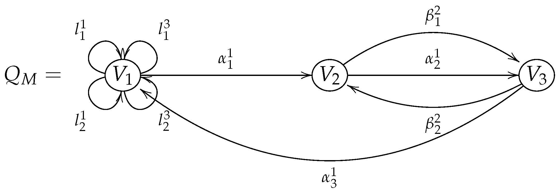
- , , , for all possible values of i and j.
- , , , , , , for all possible special cycles associated with Vertices 1, 2, and 3.
3. Main Results
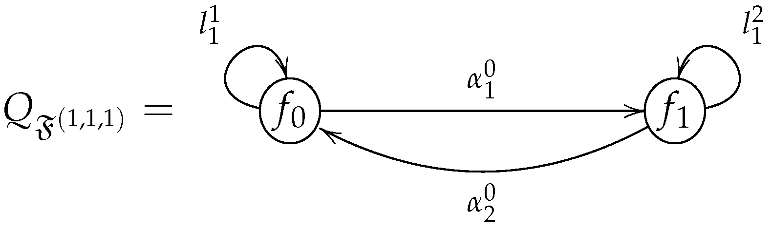
3.1. Brauer Configurations of Type
- ;
- , , for all possible values of i and j;
- , .
- ;
- ;
- ;
- .
3.2. Specializations
- They are piecewise linear and orientation-preserving.
- In the pieces where the maps are linear, the slope is a power of 2.
- Points where slopes change their values are said to be breakpoints, which are dyadic, i.e., they belong to the set , where .
4. Concluding Remarks
Future Work
- To determine braces of type associated with Thompson’s groups of type T and V.
- To determine braces based on the Cayley graph of Thompson’s group, , and V.
- To give applications of the obtained results in graph energy theory, cryptography, and coding theory.
Author Contributions
Funding
Institutional Review Board Statement
Informed Consent Statement
Data Availability Statement
Conflicts of Interest
Abbreviations
| BCA | Brauer configuration algebra |
| Dimension of a Brauer configuration algebra | |
| Dimension of the center of a Brauer configuration algebra | |
| Field | |
| Set of vertices of a Brauer configuration M | |
| Brauer message of a Brauer configuration P | |
| nth triangular number | |
| Valency of a vertex | |
| The word associated with a polygon | |
| YBE | Yang–Baxter equation |
References
- Yang, C.N. Some exact results for the many-body problem in one dimension with repulsive delta-function interaction. Phys. Rev. Lett. 1967, 19, 1312–1315. [Google Scholar] [CrossRef]
- Baxter, R.J. Partition function for the eight-vertex lattice model. Ann. Phys. 1972, 70, 193–228. [Google Scholar] [CrossRef]
- Caudrelier, V.; Crampé, N. Exact results for the one-dimensional many-body problem with contact interaction: Including a tunable impurity. Rev. Math. Phys. 2007, 19, 349–370. [Google Scholar] [CrossRef] [Green Version]
- Cedó, F.; Jespers, E.; Oniński, J. Braces and the Yang–Baxter equation. Commun. Math. Phys. 2014, 327, 101–116. [Google Scholar] [CrossRef] [Green Version]
- Nichita, F.F. Introduction to the Yang–Baxter equation with open problems. Axioms 2012, 1, 33–37. [Google Scholar] [CrossRef] [Green Version]
- Nichita, F.F. Yang–Baxter equations, computational methods and applications. Axioms 2015, 4, 423–435. [Google Scholar] [CrossRef] [Green Version]
- Massuyeau, G.; Nichita, F.F. Yang–Baxter operators arising from algebra structures and the Alexander polynomial of knots. Comm. Algebra 2005, 33, 2375–2385. [Google Scholar] [CrossRef] [Green Version]
- Kauffman, L.H.; Lomonaco, S.J. Braiding operators are universal quantum gates. New J. Phys. 2004, 6, 134. [Google Scholar] [CrossRef]
- Turaev, V. The Yang–Baxter equation and invariants of links. Invent. Math. 1988, 92, 527–533. [Google Scholar] [CrossRef]
- Rump, W. Modules over braces. Algebra Discret. Math. 2006, 2, 127–137. [Google Scholar]
- Rump, W. Braces, radical rings, and the quantum Yang–Baxter equation. J. Algebra 2007, 307, 153–170. [Google Scholar] [CrossRef]
- Ballester-Bolinches, A.; Esteban-Romero, R.; Fuster-Corral, N.; Meng, H. The structure group and the permutation group of a set-theoretical solution of the quantum Yang–Baxter equation. Mediterr. J. Math. 2021, 18, 1347–1364. [Google Scholar] [CrossRef]
- Green, E.L.; Schroll, S. Brauer configuration algebras: A generalization of Brauer graph algebras. Bull. Sci. Math. 2017, 121, 539–572. [Google Scholar] [CrossRef] [Green Version]
- Cañadas, A.M.; Gaviria, I.D.M.; Vega, J.D.C. Relationships between the Chicken McNugget Problem, Mutations of Brauer Configuration Algebras and the Advanced Encryption Standard. Mathematics 2021, 9, 1937. [Google Scholar] [CrossRef]
- Moreno Cañadas, A.; Rios, G.B.; Serna, R.J. Snake graphs arising from groves with an application in coding theory. Computation 2022, 10, 124. [Google Scholar] [CrossRef]
- Agudelo, N.; Cañadas, A.M.; Espinosa, P.F.F. Brauer configuration algebras defined by snake graphs and Kronecker modules. Electron. Res. Arch. 2022, 30, 3087–3110. [Google Scholar]
- Espinosa, P.F.F. Categorification of Some Integer Sequences and Its Applications. Ph.D. Thesis, Universidad Nacional de Colombia, Bogotá, Colombia, 2021. [Google Scholar]
- Drinfeld, V.G. On unsolved problems in quantum group theory. Lect. Notes Math. 1992, 1510, 1–8. [Google Scholar]
- Etingof, P.; Schedler, T.; Soloviev, A. Set-theoretical solutions to the quantum Yang–Baxter equation. Duke Math. J. 1999, 100, 169–209. [Google Scholar] [CrossRef] [Green Version]
- Gateva-Ivanova, T.; Van den Bergh, M. Semigroups of I-type. J. Algebra 1998, 308, 97–112. [Google Scholar] [CrossRef] [Green Version]
- Guarnieri, L.; Vendramin, L. Skew braces and the Yang–Baxter equation. Math. Comput. 2017, 85, 2519–2534. [Google Scholar] [CrossRef]
- Andrews, G.E. The Theory of Partitions; Cambridge University Press: Cambridge, UK, 2010. [Google Scholar] [CrossRef]
- da Fontoura Costa, L. Multisets. arXiv 2021, arXiv:2110.12902. [Google Scholar]
- Schroll, S. Brauer Graph Algebras. In Homological Methods, Representation Theory, and Cluster Algebras, CRM Short Courses; Assem, I., Trepode, S., Eds.; Springer: Cham, Switzerland, 2018; pp. 177–223. [Google Scholar]
- Sierra, A. The dimension of the center of a Brauer configuration algebra. J. Algebra 2018, 510, 289–318. [Google Scholar] [CrossRef]
- Belk, J.M. Thompson’s group F. Ph.D. Thesis, Cornell University, Ithaca, NY, USA, 2004. [Google Scholar]
- Burillo, J.; Cleary, S.; Stein, M.; Taback, J. Combinatorial and Metric Properties of Thompson’s Group T. Trans. Amer. Math. Soc. 2009, 361, 631–652. [Google Scholar] [CrossRef]


Disclaimer/Publisher’s Note: The statements, opinions and data contained in all publications are solely those of the individual author(s) and contributor(s) and not of MDPI and/or the editor(s). MDPI and/or the editor(s) disclaim responsibility for any injury to people or property resulting from any ideas, methods, instructions or products referred to in the content. |
© 2022 by the authors. Licensee MDPI, Basel, Switzerland. This article is an open access article distributed under the terms and conditions of the Creative Commons Attribution (CC BY) license (https://creativecommons.org/licenses/by/4.0/).
Share and Cite
Cañadas, A.M.; Ballester-Bolinches, A.; Gaviria, I.D.M. Solutions of the Yang–Baxter Equation Arising from Brauer Configuration Algebras. Computation 2023, 11, 2. https://doi.org/10.3390/computation11010002
Cañadas AM, Ballester-Bolinches A, Gaviria IDM. Solutions of the Yang–Baxter Equation Arising from Brauer Configuration Algebras. Computation. 2023; 11(1):2. https://doi.org/10.3390/computation11010002
Chicago/Turabian StyleCañadas, Agustín Moreno, Adolfo Ballester-Bolinches, and Isaías David Marín Gaviria. 2023. "Solutions of the Yang–Baxter Equation Arising from Brauer Configuration Algebras" Computation 11, no. 1: 2. https://doi.org/10.3390/computation11010002