
Chebfun Solutions to a Class of 1D Singular and Nonlinear Boundary Value Problems


Tiberiu Popoviciu Institute of Numerical Analysis, Romanian Academy, P.O. Box 68-1, 401010 Cluj-Napoca, Romania
Computation 2022, 10(7), 116; https://doi.org/10.3390/computation10070116
Submission received: 8 June 2022
/
Revised: 22 June 2022
/
Accepted: 6 July 2022
/
Published: 8 July 2022
(This article belongs to the Special Issue Mathematical Modeling and Study of Nonlinear Dynamic Processes)
Abstract
:The Chebyshev collocation method implemented in Chebfun is used in order to solve a class of second order one-dimensional singular and genuinely nonlinear boundary value problems. Efforts to solve these problems with conventional ChC have generally failed, and the outcomes obtained by finite differences or finite elements are seldom satisfactory. We try to fix this situation using the new Chebfun programming environment. However, for tough problems, we have to loosen the default Chebfun tolerance in Newton’s solver as the ChC runs into trouble with ill-conditioning of the spectral differentiation matrices. Although in such cases the convergence is not quadratic, the Newton updates decrease monotonically. This fact, along with the decreasing behaviour of Chebyshev coefficients of solutions, suggests that the outcomes are trustworthy, i.e., the collocation method has exponential (geometric) rate of convergence or at least an algebraic rate. We consider first a set of problems that have exact solutions or prime integrals and then another set of benchmark problems that do not possess these properties. Actually, for each test problem carried out we have determined how the Chebfun solution converges, its length, the accuracy of the Newton method and especially how well the numerical results overlap with the analytical ones (existence and uniqueness).
Keywords:
Chebfun; differential equation; non-linearity; singularity; convergence; Bernstein growth; improper integrals; boundary layerMSC:
65L10; 65L60; 65L70; 65D301. Introduction
The idea of solving nonlinear boundary problems as accurate as possible using spectral collocation methods is not new in the author’s work. Thus, we published the paper [1] and posted the problem [2] on the colorgreenChebfun website. In both situations, we considered nonlinear boundary value problems on the half line.
In this paper, we consider the following class of nonlinear and possible singular problems:
where
To ensure existence we will assume the following conditions are satisfied:
For the results of the existence and uniqueness of the solutions of these problems, we rely on the paper [3] and the works cited there.
We must note from the beginning that the mathematical literature abounds with such theoretical results, but their numerical illustration is often lacking. We want to fill this gap as much as possible.
Notice that f may not be a Caratheodory function because of the singular behavior of the u variable, i.e., f may be singular at . Problems of the above form have been discussed extensively in the literature usually when reduces to with (see for instance [4]).
The main purpose of our study is to solve numerically such problems as accurately as possible.
In general, attempts are made to attenuate singularity by algebraic manipulations, but these, along with non-linearities, raise serious problems for any numerical algorithm.
Traditionally, they have been overcome using variants of the shooting method. We will never resort to such methods. As the methods with finite differences, finite elements or volumes, or conventional ChC have shown their limits, we want to show that the use of Chebfun variant of ChC method can address most of these issues.
The work has the following structure. In Section 2, we elaborate a brief comparison between Chebfun and the conventional ChC method. The core of the paper is Section 3. Here, we report the numerical results of solving eight problems with varying degrees of non-linearity and even singularity. In each case, we establish the type of convergence of the Chebyshev collocation method implemented with Chebfun. In Section 4, we draw some conclusions on the usefulness and performance of the Chebfun system. We believe that additional experiments are needed in order to draw even firmer conclusions.
2. Chebfun vs. Conventional ChC Method
Feel symbolic but run at the speed of numerics! [5].
This quote contains the essence of the Chebfun system. It is implemented in object-oriented MATLAB and has been introduced in 2004. The algorithms involved amount to spectral collocation methods on Chebyshev grids of automatically determined resolution.
In a latter extension, the chebop class has been introduced (see [6]). We extensively use the codes from this class. In [6] the authors observe that “the central principle of the Chebfun system is to evaluate functions in sufficiently many Chebyshev points for a polynomial interpolant to be accurate to machine precision”.
The chebop system is implemented by means of four MATLAB classes, namely: domain, chebop, oparray, and varmat, where the last two classes are not normally relevant at user level. Instead, at the user level one has to specify the domain ( being default), the differential operator along with boundary conditions such that the boundary value problem is well defined, and possible initial guess for Newton’s method. Such a Chebfun code contains only a few lines, it is very intuitive and delivers very valuable output parameters relative to the convergence of the method and the evolution of Newton iterations.
Chebfun normally represents solutions to BVPs by polynomial approximations, typically with an accuracy of about 10 digits, whose degree N (the resolution) may be quite high (actually ). Due to the bad conditioning of Chebyshev differentiation matrices, on a usual computing station the maximum N one can hope for is around 1000. The polynomials can be interpreted as interpolants through a sufficiently large number of samples at Chebyshev points defined by
From this representation of the solution starts the essential difference from conventional ChC. In the case of the second method, it is impossible to establish this resolution apriori. Thus, although the Chebyshev collocation remains one and the same method, there are some algorithmic advancements incorporated in Chebfun. We only mention the concept of quasi-matrix, chopping algorithm, lazy evaluation, to name just a few.
Moreover, implementing conventional ChC is a much more laborious thing as it appears for instance from our work [1]. First of all, it is a challenging matter of establishing the right resolution. In most cases, this is reduced to repeated tests. Imposing less common boundary conditions (mixed or non-local) is another “thorny”issue. Finally, obtaining output parameters similar to those provided by Chebfun requires additional effort, such as a fast Chebyshev transform.
Chebfun’s code is open source and available on Github, https://github.com/chebfun/chebfun, last accessed date 15 February 2022.
3. Numerical Results
3.1. A Test Problem with Known Solution
The exact solution is known. It reads
Among other phenomena, this problem models conductive heat transfer with nonlinear heat generation.
It is important to state that Chebfun works in the physical (values) space, i.e., computes the nodal values of a solution in the nodes defined by (3). At the same time it computes the values of the coefficients of the solution expansion in phase (coefficients) space. The latter reads
where are the usual Chebyshev polynomials and N is the length of the solution provided by Chebfun.
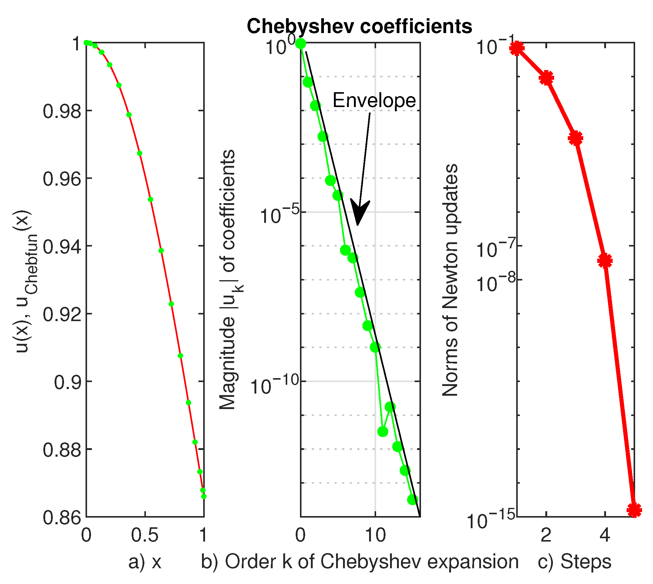
The Chebfun solution to this problem is depicted in panel (a) of Figure 1. It is clear that it perfectly overlaps with the exact solution. The error in the norm is of the order .
The second panel of this figure shows that the Chebyshev coefficients of the solution decrease almost linearly to the machine precision and the length of solution is . A straight line which bounds them from above, the so called envelope, is also drawn. This parallelizes the straight line through origin of the equation
where It means that the (asymptotic) rate of convergence of Chebfun is exponential or geometric (see the monograph [9], Chapter 2 for the definition of the rate of convergence).
From panel (c) of the same figure, we understand that the Newton method is of the second order and uses five iterations.
Chebfun provides precise details on the accuracy with which the boundary conditions are enforced. In this case the residue vanishes.
In [7] a classic method with finite differences is used in order to solve this problem and the authors expect an accuracy of order In a recent paper [8], the authors make use of the Haar wavelet method in order to solve a quasi-linearized version of this problem. Nor do they expect for better accuracy than something of order
Finally, we solved the problem with MATLAB’s bvp4c routine (see [10] for this routine). In this case we could not find the solution with an error better than
Due to limited space, we are not able to repeat and report all these comparisons for every problem which follows. However, we will sum up conclusions in the last section.
3.2. A Bernstein Type Boundary Value Problem
In [11], the authors consider a problem of type (1) in which the nonlinear term f satisfies the so called Bernstein growth condition. Actually, it means that f can grow at most quadratically in its derivative variable.
We consider the following example from this paper:
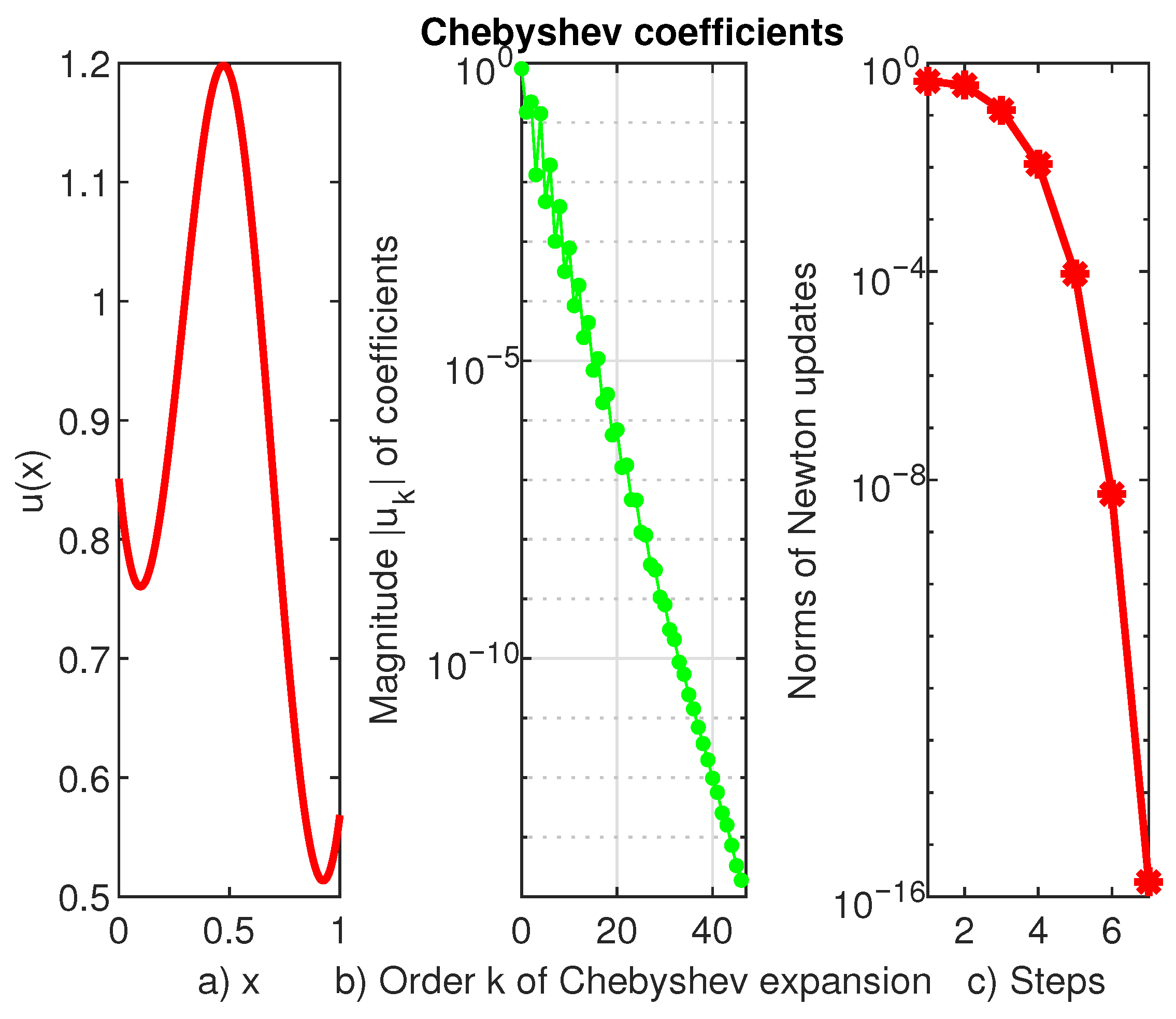
The Chebfun solution to this problem is depicted in panel (a) of Figure 2. This has exactly the same shape as the one obtained in [11] by shooting along with continuation with respect to the initial data. The Newton’s method in solving the Chebfun discretization has second order (see panel (b)) and the coefficients of Chebfun solution decrease smoothly and linearly to the level of machine precision. The convergence of the method remains exponential but the slope m approximately equals in (7), i.e., less optimal than in the previous example.
We have intentionally chosen this example from the paper quoted above to show that the enforcement of mixed conditions is extremely simple in Chebfun and especially very precise, i.e., the final error in solving them is of order . Such an estimate is practically impossible with conventional ChC or bvp4c.
3.3. Lane-Emden Equation of the Second Kind
The equations of Lane-Emden-Fowler type arise in various applications in mechanics, nuclear physics, gas-dynamics, stellar structures, and chemically reacting systems. In [12], the author considers the nonlinear ODE
supplied with boundary conditions
or
For and the problems (9) and (10) admits the following exact first integral
where and denotes the exponential integral
In order to see how accurate this integral is satisfied we take first and and then from the boundary conditions we introduce and (the symmetry of solution with respect to x). The values and have been computed by Chebfun.
Thus, in our computation, regardless of the values of parameters and , the first integral (12) is satisfied with a precision of order
Chebfun has no difficulty solving problems (9)–(11). The solutions to the problems (9) and (10) are displayed in Figure 3. The Newton method has effectively second order and no more than two or three iterations are used in each case.
The convergence of the method is exponential with the slope m approximately equaling in (7). Improper integrals
in the first integral (12) are also calculated without any difficulty by Chebfun. It uses sum operator along with option ‘splitting’, ‘on’. In each case, the Newton process started from the initial guess .
3.4. A Singular Problem from the Theory of the Pseudo-Plastic Fluids
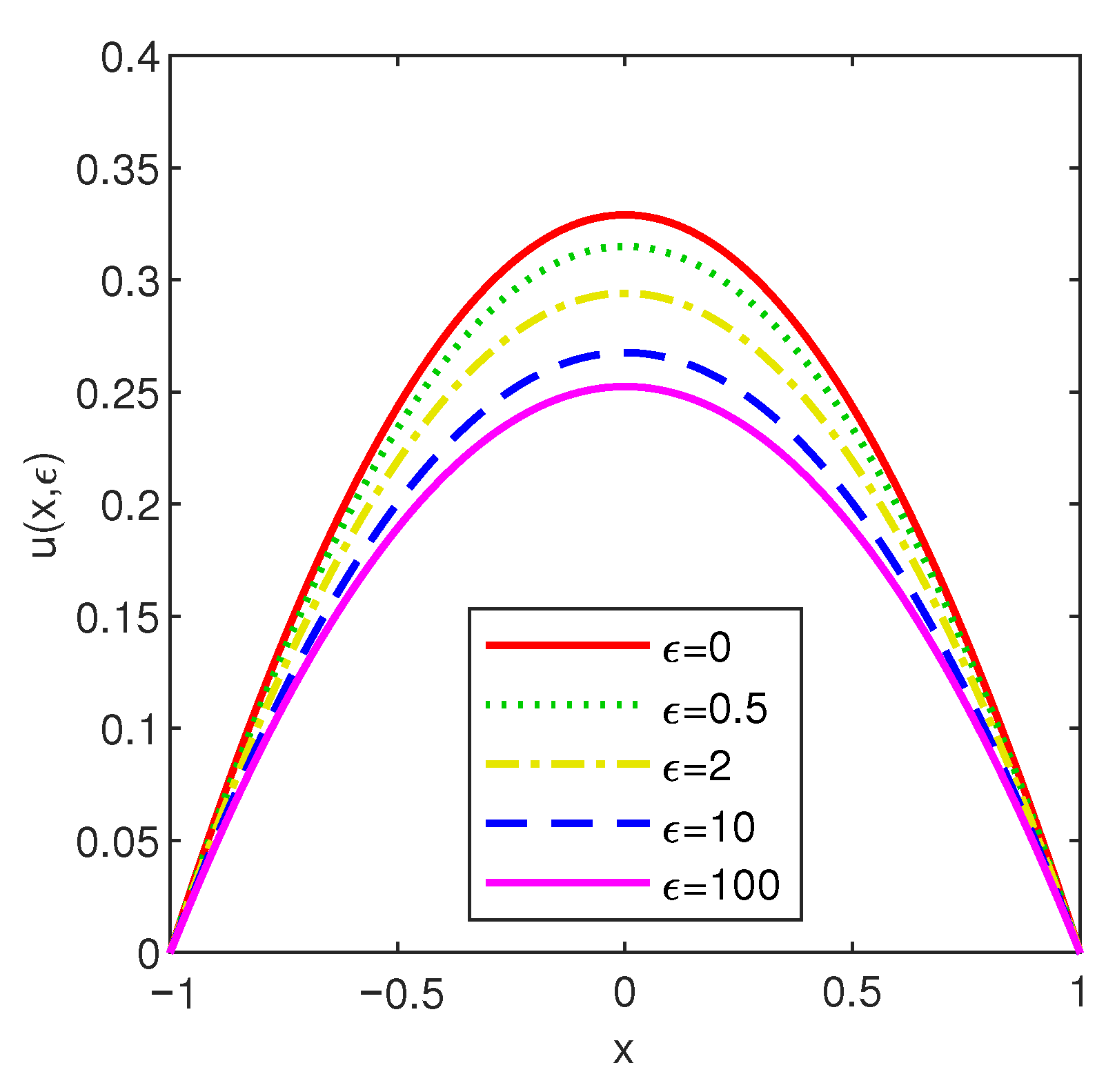
In [13], the authors consider the existence issue for the problem
where The case corresponds to the Newtonian fluid.
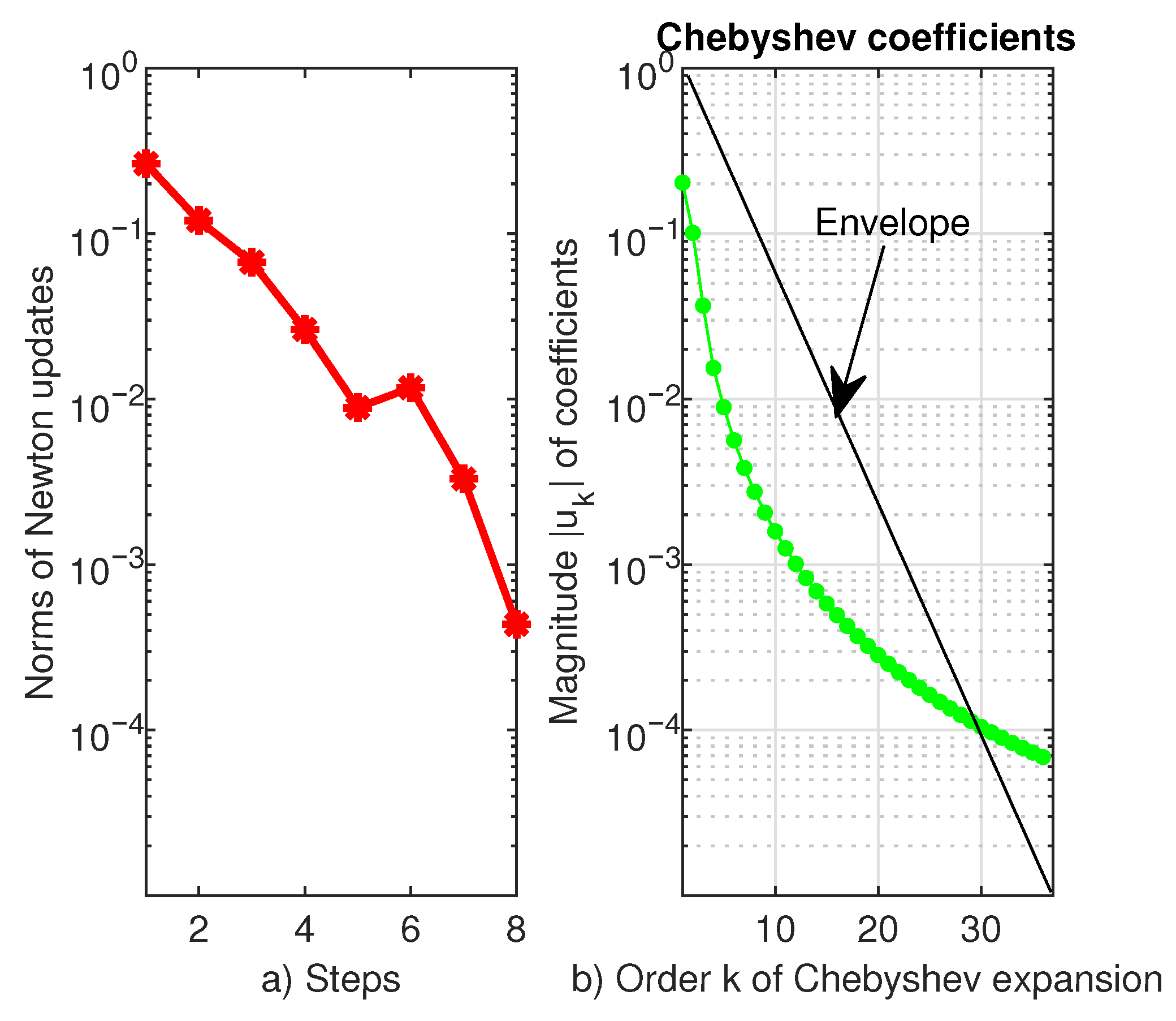
This problem is much more difficult than the previous one in the following sense. If, in the previous case, Chebfun used a tolerance of order for Newton’s solver in this case we had to loosen this tolerance to in order to guarantee a convergent procedure.
In the left panel of Figure 5, we display the norm of Newton’s updates vs. iteration number in the worst case, i.e., . It is apparent that the order of the Newton’s method is much less than 2.
From the right panel of Figure 5 we see that the solution has length 37 and its coefficients decrease smoothly but remain very far from the machine precision level. We also drew the envelope for these coefficients and from the log-linear plot (b) of Figure 5 we can only infer that asymptotically, i.e., for large k, the coefficients of expansion (6) of solution satisfy
which means that the rate of convergence is only algebraic.
The point where the envelope intersects the coefficients’ curve is (roughly!) the magnitude of the error. In fact, the coefficients decrease slightly below the level
The problem of finding an initial guess in order to ensure the convergence of Newton’s iterates is not at all simple in this case. Repeated attempts led us to an initial date of the form
This initial guess satisfies the boundary conditions of problem (13) and has a curvature close to that of numerical outcomes.
It should be noted that for values of the parameter in the range (0, 1/2) Chebfun completely failed!
In order to solve this problem for arbitrary values of in [14] the authors have introduces an iterative technique which reduces the problem to a sequence of usual eigenvalue problems. We have tested the capabilities of Chebfun in solving various Sturm–Liouville problems in some previous papers thus we are not interested in these iterative techniques (see for instance our contribution [15]).
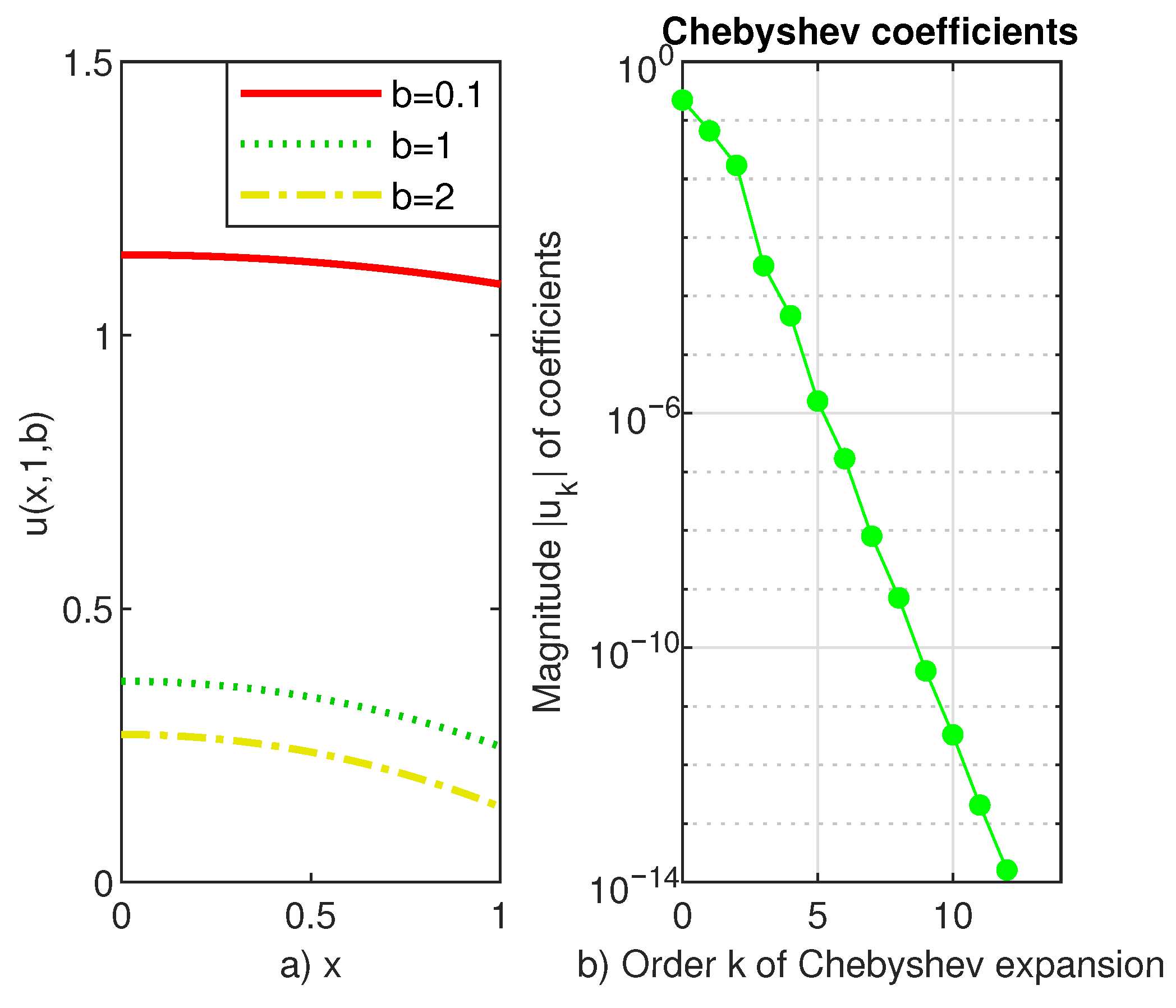
3.5. A Nonlinear Heat Conduction Model of the Human Head
The analytical study of the problem
has been initiated in [16]. Roughly speaking in this model the right hand side is the heat production rate per unit volume, is the absolute temperature, x is the radial distance from the centre, a is the inverse of the average thermal conductivity inside the head and b is a heat exchange coefficient.
Three solutions of this problem are reported in the panel (a) of Figure 6.
The behavior of Chebyshev coefficients in the panel (b) of Figure 6 shows that the rate of convergence is definitely exponential.
Although the problem has received some attention over time, we have not found numerical results with which to compare ours. In any case, in its solution Newton’s method keeps the second order and does not use more than six iterative steps.
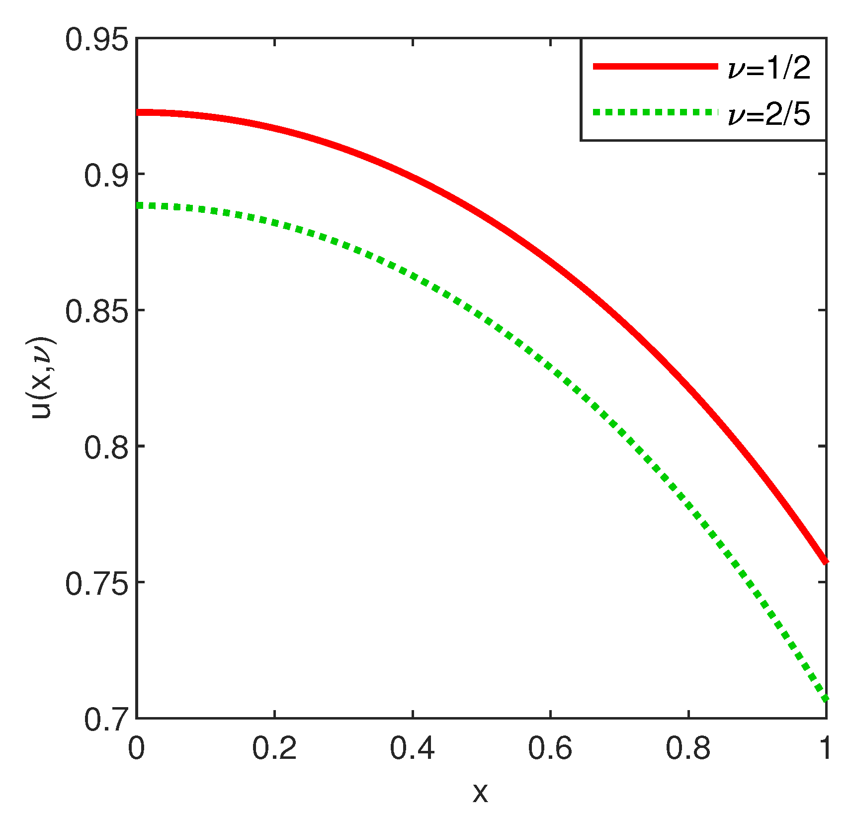
3.6. Membrane Buckling
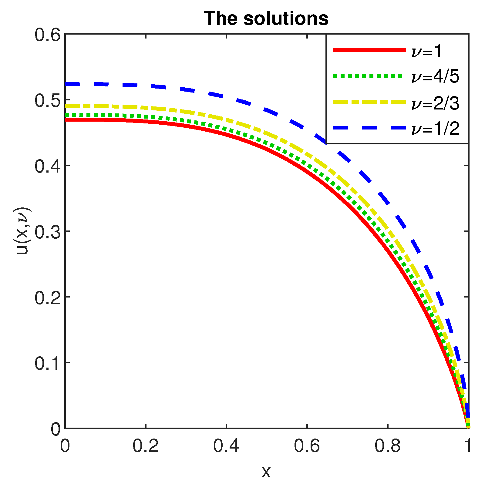
In [17] the authors consider, among other problems, the following nonlinear and singular problem:
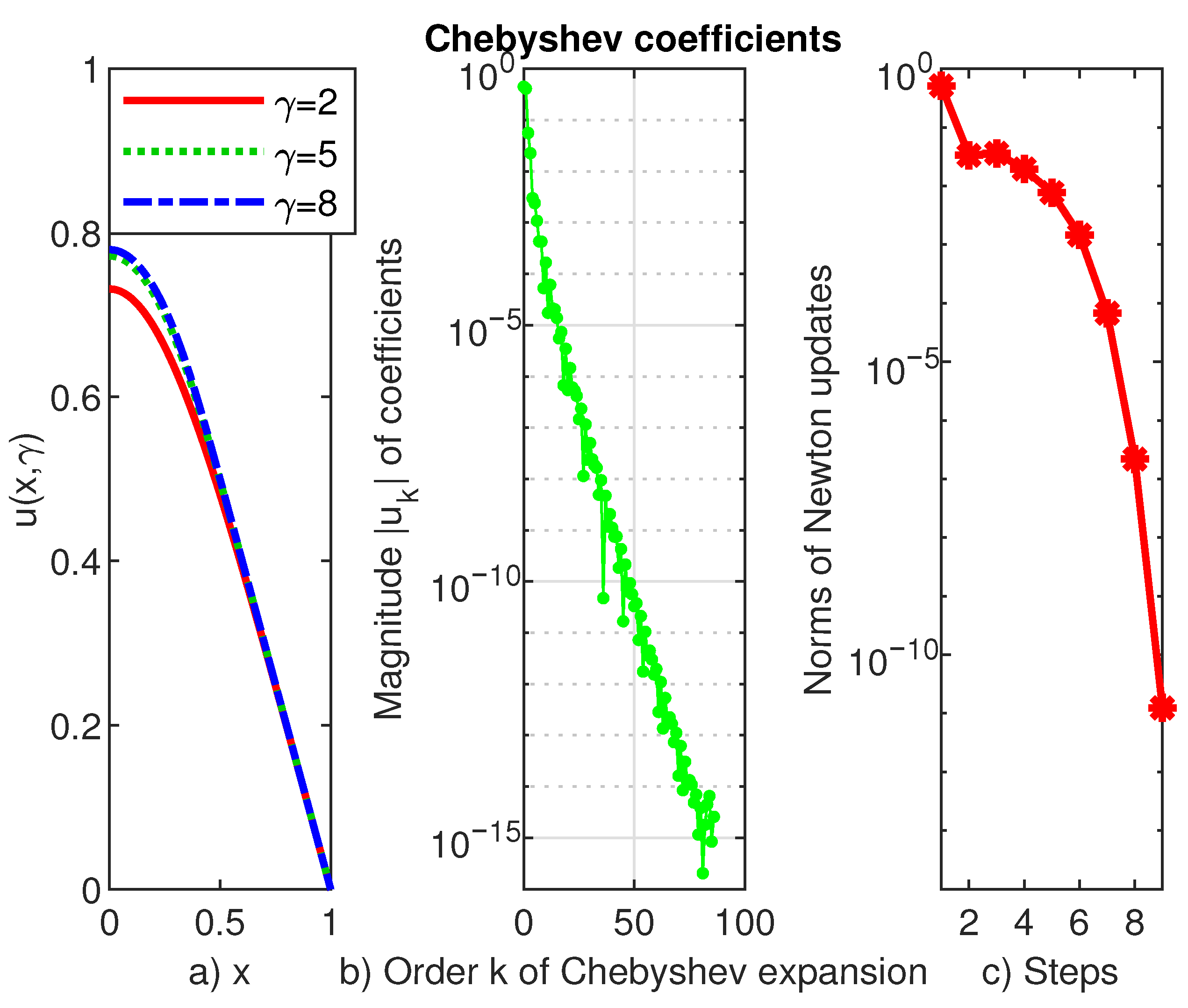
which describes a flat, circular elastic membrane which is deformed by an axisymmetric pressure applied to its surface. The edge of the membrane is restrained from deforming normal to its mid-plane. Either a compressive radial thrust or a contractile radial displacement is applied to the edge. The dependent variable stands for the radial stress and x is the dimensionless radius. The parameter stands for Poisson ration of the membrane material.
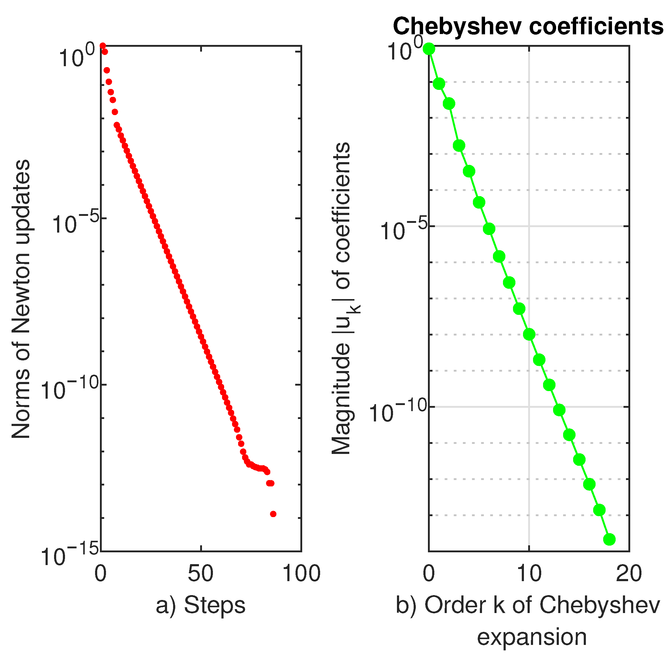
The calculation of the two solutions differs fundamentally. In the first case () Chebfun produces the solution in five iterations and the Newton’s method has the second order. In the other case, Chebfun produces the solution in 86 iterations and the order of Newton’s method is far from order two. This aspect is visible in the left panel of Figure 8.
The behavior (almost linear decrease to the machine precision level) of the Chebyshev coefficients of the solution suggests a still exponential convergent process (see the (b) panel in Figure 8).
One remark is suitable at this stage. For lower values of the Poison parameter (membrane made of stiffer materials), Chebfun simply failed.
3.7. A Nonlinear (Super-Linear) Singular Problem
Our observations from many numerical experiments lead us to the conclusion that singularity is more difficult to manage than non-linearity for Chebfun. In order to strengthen this assertion we consider another example.
Thus, in [18] the authors are concerned the singular and non-linear problem:
Three solutions of this problem are displayed in the panel (a) of Figure 9.
For higher values of than 1, Chebfun could not solve the problem even though the tolerance was considerably lower. This is not the case for the exponent .
For the highest value of , the convergence rate remains exponential and the Newton’s method has an order close to two. These result from panels (b) and (c) of the same figure.
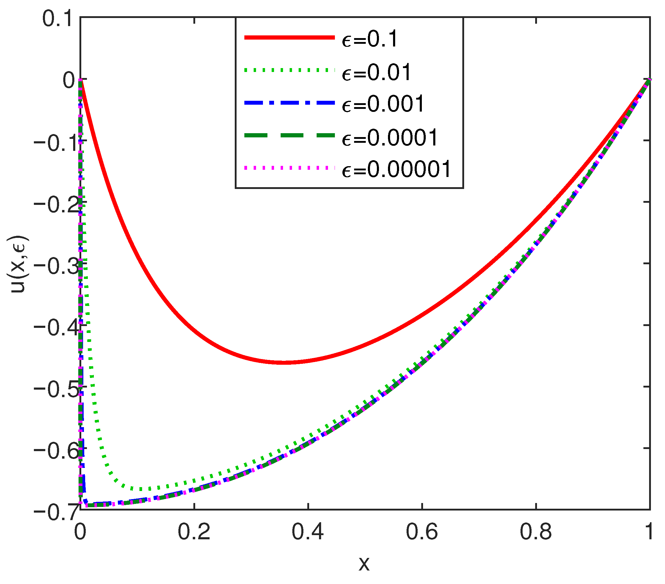
3.8. A Singularly Perturbed Nonlinear Problem
In [19] the authors analyze the following problem:
Five solutions of this problem are reported in Figure 10. They correspond to
and confirm that there exists a sharp boundary layer at the right of
In order to reach the lowest value we have used continuation with respect to this parameter and we have loosen the tolerance to As a result, the convergence of the Newton method is no longer quadratic but is reduced to something around the unit.
It is very important to underline that for Chebfun uses a solution of length 97 and for : it uses a much larger solution of length The Newton’s method resolved the first case mentioned above using 7 iterations while for the later case it resolved the problem only in four iterations. The order of the Newton method is close to two, but the Chebyshev coefficients of the solution decrease only to the level
We have not found numerical results in the literature to compare with ours. Some other listed problems in [19] have been solved by Chebfun without any difficulty.
The exact solution to (17) has the form:
When : the infinity norm of the error
reaches the value of order which emphasizes the accuracy of the computations.
4. Discussion
Chebfun is not a universal panacea!
There are nonlinear and singular problems for which no matter how much we have reduced tolerance, i.e., bvpTol, Chebfun fails. An example is the problem (13). This seems to be the most difficult problem in the multitude of our numerical experiments.
The exponential accuracy is proved by the rate the Chebyshev coefficients of solutions decay. Again the problem (13) is in the worst situation. The rate of convergence is only algebraic. A slightly better situation is found relative to the singular problem (15). Otherwise, in all other cases, the problems are solved with exponential accuracy.
Another advantage of Chebfun compared to conventional ChC is the lack of rounding-off plateau in the analysis of solution coefficients. This is due to the way Chebfun truncates.
The main conclusion of the paper is that, up to date, collocation in form of Chebfun provides the most accurate solution in solving genuinely nonlinear and/or singular 1D BVPs.
We believe that the complete treatment of these difficult BVPs, until finding the effective order of accuracy of numerical methods, shows current limitations of numerical analysis.
Funding
This research received no external funding.
Data Availability Statement
Samples of the Chebfun codes are available from the author by request.
Acknowledgments
The author would like to thank the Computation editors for their careful collaboration and the reviewers for their comments. These comments considerably improved the paper.
Conflicts of Interest
The author declares no conflict of interest.
Abbreviations
The following abbreviations are used in this manuscript:
| BVP | Boundary Value Problem |
| ChC | the Chebyshev collocation method |
| Chebfun | is a software system in object-oriented MATLAB; |
| it extends many MATLAB operations on vectors and matrices to functions and operators; | |
| it is compatible with MATLAB 7.9 (R2009b) or later | |
| 1D | one-dimensional |
| tilde | asymptotic equivalence |
References
- Gheorghiu, C.I. Pseudospectral solutions to some singular nonlinear BVPs. Numer. Algor. 2015, 68, 1–14. [Google Scholar] [CrossRef]
- Gheorghiu, C.I. A Third-Order Nonlinear BVP on the Half-Line. Available online: https://www.chebfun.org/examples/ode-nonlin/GulfStream.html (accessed on 30 January 2020).
- Agarwal, R.P.; O’Regan, D. A singular Homann differential equation. ZAMM Z. Angew. Math. Mech. 2003, 83, 344–350. [Google Scholar] [CrossRef]
- Agarwal, R.P.; O’Regan, D. Singular initial and boundary value problems with sign changing nonlinearity. IMA J. Appl. Math 2000, 65, 173–198. [Google Scholar] [CrossRef]
- Trefethen, L.N.; Birkisson, A.; Driscoll, T.A. Exploring ODEs; SIAM: Philadelphia, PA, USA, 2018; pp. 51–62. [Google Scholar]
- Driscoll, T.A.; Bornemann, F.; Trefethen, L.N. The chebop system for automatic solution of differential equations. Bit Numer. Math. 2008, 48, 701–723. [Google Scholar] [CrossRef]
- Russell, R.D.; Shampine, L.F. Numerical methods for singular boundary value problems. SIAM J. Numer. Anal. 1975, 12, 13–36. [Google Scholar] [CrossRef]
- Singh, R.; Guleria, V.; Singh, M. Haar wavelet quasi-linearization method for numerical solution of Emden–Fowler type equations. Math. Comput. Simul. 2020, 174, 123–133. [Google Scholar] [CrossRef]
- Boyd, J.P. Chebyshev and Fourier Spectral Methods, 2nd ed.; Dover: Mineola, NY, USA, 2001; pp. 19–57. [Google Scholar]
- Kierzenka, J.; Shampine, L.F. A BVP solver based on residual control and the Maltab PSE. ACM Trans. Math. Softw. 2001, 27, 299–316. [Google Scholar] [CrossRef]
- Granas, A.; Guenther, R.B.; Lee, J.W. Continuation and shooting methods for boundary value problems of Bernstein type. J. Fixed Point Theory Appl. 2009, 6, 27–61. [Google Scholar] [CrossRef]
- Van Gorder, R.A. Exact fist integral for a Lane-Emden equation of the second kind modeling a thermal explosion in a rectangular slab. New Astron. 2011, 16, 492–497. [Google Scholar] [CrossRef]
- Agarwal, R.P.; O’Regan, D. Singular Problems Modelling Phenomena in the Theory of Pseudoplastic Fluids. ANZIAM J. 2003, 45, 167–179. [Google Scholar] [CrossRef] [Green Version]
- Flagg, R.C.; Luning, C.D.; Perry, W.L. Implementation of New Iterative Techniques for Solutions of Thomas-Fermi and Emden-Fowler Equations. J. Comput. Phys. 1980, 38, 396–405. [Google Scholar] [CrossRef]
- Gheorghiu, C.-I. Accurate Spectral Collocation Computation of High Order Eigenvalues for Singular Schrödinger Equations. Computation 2021, 9, 2. [Google Scholar] [CrossRef]
- Duggan, R.C.; Goodman, A.M. Pointwise Bounds for a Nonlinear Heat Conduction Model of the Human Head. Bull. Math. Biol. 1986, 48, 229–236. [Google Scholar] [CrossRef]
- Callegari, A.J.; Reiss, E.L.; Keller, H.B. Membrane Buckling: A Study of Solution Multiplicity. Commun. Pure Appl. Math. 1971, 24, 499–527. [Google Scholar] [CrossRef]
- Agarwal, R.P.; O’Regan, D. Nonlinear Super-linear Singular and Non-singular Second Order Boundary Value Problems. J. Differ. Equ. 1998, 143, 60–95. [Google Scholar] [CrossRef] [Green Version]
- Mazzia, F.; Sgura, I. Numerical approximation of nonlinear BVPs by means of BVMs. Appl. Numer. Math. 2002, 42, 337–352. [Google Scholar] [CrossRef]
Figure 1.
(a) The exact solution (5) (green dots) and Chebfun solution (6) to problem (4) are displayed. (b) In a log-linear plot the behaviour of Chebyshev coefficients of solution to problem (4) (green dots) is reported. The envelope is depicted by a black straight line. (c) This panel shows that Newton’s method is of second order and uses five iterative steps.

Figure 2.
(a) The Chebfun solution to problem (8) is depicted. (b) In this panel we report the behaviour of Chebyshev coefficients of solution to problem (8) when . (c) Newton’s method appears to be of second order and uses seven iterative steps.


Figure 4.
Chebfun solutions to problem (13) for various values of .
Figure 4.
Chebfun solutions to problem (13) for various values of .

Figure 5.
(a) The convergence of Newton’s method in solving problem (13) when . (b) In a log-linear plot we display the decreasing behavior of the Chebyshev coefficients (green dots) of solution to the same problem.
Figure 5.
(a) The convergence of Newton’s method in solving problem (13) when . (b) In a log-linear plot we display the decreasing behavior of the Chebyshev coefficients (green dots) of solution to the same problem.

Figure 6.
(a) Three solutions to the problem (14). (b) This panel shows that when b: the Chebyshev coefficients of solution decrease almost linearly, close to the machine precision level, with a slope a little bit larger than .
Figure 6.
(a) Three solutions to the problem (14). (b) This panel shows that when b: the Chebyshev coefficients of solution decrease almost linearly, close to the machine precision level, with a slope a little bit larger than .

Figure 7.
Two solutions to the problem (15).
Figure 7.
Two solutions to the problem (15).

Figure 8.
(a) The norm of the Newton’s updates when Chebfun computes the solution . (b) The Chebyshev coefficients of solution to problem (15) with .
Figure 8.
(a) The norm of the Newton’s updates when Chebfun computes the solution . (b) The Chebyshev coefficients of solution to problem (15) with .

Figure 9.
(a) Three solutions to the problem (16) when . (b) This panel shows that when the Chebyshev coefficients of solution decrease almost linearly close to the machine precision with a slope a little bit larger than . (c) Newton updates are illustrated for the same value of
Figure 9.
(a) Three solutions to the problem (16) when . (b) This panel shows that when the Chebyshev coefficients of solution decrease almost linearly close to the machine precision with a slope a little bit larger than . (c) Newton updates are illustrated for the same value of

Figure 10.
Five solutions to problem (17) for various values of the parameter .
Figure 10.
Five solutions to problem (17) for various values of the parameter .

Publisher’s Note: MDPI stays neutral with regard to jurisdictional claims in published maps and institutional affiliations. |
© 2022 by the author. Licensee MDPI, Basel, Switzerland. This article is an open access article distributed under the terms and conditions of the Creative Commons Attribution (CC BY) license (https://creativecommons.org/licenses/by/4.0/).
Share and Cite
MDPI and ACS Style
Gheorghiu, C.-I. Chebfun Solutions to a Class of 1D Singular and Nonlinear Boundary Value Problems. Computation 2022, 10, 116. https://doi.org/10.3390/computation10070116
AMA Style
Gheorghiu C-I. Chebfun Solutions to a Class of 1D Singular and Nonlinear Boundary Value Problems. Computation. 2022; 10(7):116. https://doi.org/10.3390/computation10070116
Chicago/Turabian StyleGheorghiu, Călin-Ioan. 2022. "Chebfun Solutions to a Class of 1D Singular and Nonlinear Boundary Value Problems" Computation 10, no. 7: 116. https://doi.org/10.3390/computation10070116
Note that from the first issue of 2016, this journal uses article numbers instead of page numbers. See further details here.