Article

Balanced Circular Packing Problems with Distance Constraints

by
Tetyana Romanova
1,2,
Olexandr Pankratov
1,2,
Igor Litvinchev
3,
Petro Stetsyuk
4,
Oleksii Lykhovyd
4,
Jose Antonio Marmolejo-Saucedo
5,* and
Pandian Vasant
6
1
Department of Mathematical Modeling and Optimal Design, A. Pidhornyi Institute for Mechanical Engineering Problems, National Academy of Sciences of Ukraine, 61046 Kharkiv, Ukraine
2
Department of Systems Engineering, Kharkiv National University of Radioelectronics, 14 Nauky Ave., 61166 Kharkiv, Ukraine
3
Faculty of Mechanical and Electrical Engineering, Nuevo Leon State University (UANL), Av. Universidad s/n, Col. Ciudad Universitaria, San Nicolas de los Garza 66455, Mexico
4
Department of Nonsmooth Optimization Methods, V. Glushkov Institute of Cybernetics, National Academy of Sciences of Ukraine, 40 Academika Glushkova Ave., 03187 Kyiv, Ukraine
5
Facultad de Ingenieria, Universidad Panamericana, Augusto Rodin 498, Ciudad de Mexico 03920, Mexico
6
Modeling Evolutionary Algorithms Simulation & Artificial Intelligence (MERLIN), Faculty of Electrical & Electronic Engineering, Ton Duc Thang University, Ho Chi Minh City 700000, Vietnam
*
Author to whom correspondence should be addressed.
Computation 2022, 10(7), 113; https://doi.org/10.3390/computation10070113
Submission received: 5 April 2022 / Revised: 20 June 2022 / Accepted: 30 June 2022 / Published: 4 July 2022
(This article belongs to the Special Issue Intelligent Computing, Modeling and its Applications)

Abstract

:
The packing of different circles in a circular container under balancing and distance conditions is considered. Two problems are studied: the first minimizes the container’s radius, while the second maximizes the minimal distance between circles, as well as between circles and the boundary of the container. Mathematical models and solution strategies are provided and illustrated with computational results.

1. Introduction

The circular packing problem (CPP) consists of placing several circles in a larger object called a container. The circles must be arranged without mutual overlapping (the non-overlapping condition) and completely inside the container (the containment condition). CPPs (including CPPs in non-Euclidean geometry) form a broad category at the boundary between computational geometry and combinatorics [1,2,3]. The optimized CPP aims to find “the best” layout, e.g., maximizing the space utilization of the container or minimizing the size of the container. Optimized CPPs have multiple applications in logistics and production planning, biology and medicine, chemistry and additive manufacturing [4,5,6].
Various types of CPP can differ according to circle sizes (different or equal) [4,7,8,9] and container shapes (circles or polyhedrons) [10,11,12]. In open-dimension CPPs, the shape of the container is typically fixed, while the size is optimized [13,14]. The problem of packing circles into containers with prohibited zones is considered in [15,16,17,18]. Prohibited zones typically result in non-convex, multiconnected and/or disconnected containers.
Additional constraints motivated by applications can be introduced. For example, in a satellite module layout design, equilibrium/balance constraints are imposed to assure the proximity of the gravity center of the container to the corresponding center of the circles [19,20,21,22,23]. In many applications, CPPs are formulated for circles defined in non-Euclidean norms [17,24,25]. Nesting, i.e., the stacking of circular disks one over another, can also be considered [26,27,28,29,30].
Solution approaches to CPPs can be roughly divided into four large classes [4,6,31]. The techniques of the first group are based on nonlinear programming formulations of the CPP, and these approaches apply different exact or approximation methods for this class of optimization problems [5,11,12,15,20,21]. The second class of approaches is based on tessellating or approximating the container with a finite grid [24,26,32,33,34]. Then, the CPP is approximately reduced to a large-scale discrete programming problem in order to assign the centers of the circles to grid nodes. Using metaheuristic techniques for CPPs forms the third class of approaches [35,36]. The last group is represented by hybrid approaches combining the algorithmic ideas of the previous groups [7,8,10,13,14,19,28,31]. A collection of benchmark problem instances and corresponding best-known solutions is presented on E. Specht’s website [37], specifically for the problem of packing circles into various containers.
The objective in most optimized packing problems is to find the densest possible packing arrangement, e.g., maximizing the occupation of the container or finding the minimal container for an open-dimension problem. However, in many up-to-date applications, the dense packing concept must be revised.
In sparse packing [38], the distance between the objects, as well as between the objects and the container, must be sufficiently large. In container-loading applications, these conditions arise to facilitate access to the objects during loading/unloading. Generating lightweight void structures by 3D printing requires sufficient distance between the voids to assure the mechanical strength of the part [39]. Sparse packing arises in thermal deburring, which is a state-of-the-art technology for cleaning 3D-printed parts of non-sintered powder particles [38]. The burrs are removed from 3D objects by exploding gas mixtures in a closed chamber. To achieve a reasonable processing quality and a “uniform” distribution of power and thermal effects, the parts must be placed at sufficient distances from one another.
In this work, the packing of different circles in a circular container under balancing and distance conditions is considered. Dense and sparse formulations are studied. The first problem aims to minimize the container’s radius. In the second, the minimal distance between circles, and between the circles and the container’s boundary, is maximized.

2. Dense Packing Circular Problem with Distance and Balancing Conditions

In this section, a circular packing problem is studied under balancing and distance conditions. The objective is to obtain the smallest possible circular container (dense packing).
Let S i , i = 1 , 2 , , n be a family of circles with radii r i and weights w i . Let S be an external circle (container) centered at the origin and having radius r. By the definition, the center of gravity of the circle S is also located at the origin. Denote by ( x i , y i ) the unknown center coordinates of S i , and let x = ( x 1 , x 2 , , x n ) and y = ( y 1 , y 2 , , y n ) .
Let ρ i j > 0 be the minimum permitted distance between S i and S j , 1 i < j n . In addition, let ρ i > 0 be the minimum permitted distance between S i and the boundary of the object S * = R 2 \ int S , i = 1 , , n . More specifically, let
d i s t ( S i ( v i ) , S j ( v j ) ) ρ i j ,   1 i < j n ,   d i s t ( S i ( v i ) , S * ) ρ i ,   i = 1 , , n  
where d i s t ( A , B ) = m i n a A , b B d i s t ( a , b ) and d i s t ( a , b ) refer to the (Euclidean) distance between two points a and b .
A dense circular balanced packing (DCBP) problem can be stated as follows. Pack the circles S i , i = 1 , 2 , , n in a minimum-radius circular container S subject to the distance constraints in (1), such that the gravitation center of the family of circles S i , i = 1 , 2 , , n is located at the origin (i.e., coincides with the gravity center of S).
A trivial lower bound on the minimal radius of S is
r l o w = m a x i = 1 , , n r i + ρ , ρ = max { m a x i = 1 , , n ρ i , 0.5 m a x 1 i < j n ρ i j }
The DCBP is stated as a nonlinear optimization problem in R 2 n + 1 :
r * = min r , x , y r
subject to
( x i x j ) 2 + ( y i y j ) 2 ( r i + r j + ρ i j ) 2 , 1 i < j n ,  
x i 2 + y i 2 ( r r i ρ i ) 2 , i = 1 , , n ,
i = 1 n λ i x i = 0 , i = 1 n λ i y i = 0 ,
r r l o w
where λ i = w i / j = 1 n w j .
The constraints in (3) guarantee that the distance between the pair of circles S i and S j is at least ρ i j , 1 i < j n , while the constraints in (4) assure that the distance between S i and the boundary of S is at least ρ i   i = 1 , 2 , , n . The linear constraints in (5) state that the gravity center of the family S i , i = 1 , 2 , , n coincides with the origin, while the “dummy” constraint in (6) provides the lower bound for the objective value.

2.1. Sequential Algorithm for DCBPs

Using penalty functions, the problem in (1)–(5) can be transformed into the unconstrained minimization of a non-smooth function
m i n r , x , y { f ( r , x , y ) = r + Φ P ( r , x , y ) }  
where the penalty function Φ P ( r , x , y ) has the form
Φ P ( r , x , y ) = P 1 F 1 ( r , x , y ) + P 2 F 2 ( x , y ) + P 3 max { 0 , r + r l o w }  
Here P = { P 1 , P 2 , P 3 } , where the penalization coefficients P k , k = 1 , 2 , 3 are positive, and the functions F 1 ( r , x , y ) and F 2 ( x , y ) are as follows:
F 1 ( r , x , y ) = i = 1 n max { 0 , x i 2 + y i 2 ( r r i ρ i ) 2 } + i = 1 n j = i + 1 n max { 0 , ( x i x j ) 2 ( y i y j ) 2 + ( r i + r j + ρ i j ) 2 }
F 2 ( x , y ) = max { 0 , i = 1 n λ i x i , i = 1 n λ i x i } + max { 0 , i = 1 n λ i y i , i = 1 n λ i y i } ,
The local minimization in (2)–(6) is equivalent to the local minimization in the unconstrained non-smooth problem in (7)–(10). If Φ P ( r , x , y ) = 0 in the local minimum of the function f ( r , x , y ) for certain values of the coefficients P = { P 1 , P 2 , P 3 } , then this point is also a local minimum for the problem in (2)–(6). The choice of the penalty coefficients P 1 , P 2 and P 3 allows the adjustment of the violation of the constraints in (3)–(6). The coefficient P 1 corresponds to the “total violation” of the quadratic constraints in (3)–(4), P 2 “controls” the linear constraints in (5), while P 3 adjusts the constraint in (6).
The sequential algorithm to obtain the best local solution to the problem in (2)–(6) uses the multistart method with randomly selected starting points and is based on a variant of Shor’s r-algorithm (see, e.g., [40,41,42,43] and Appendix A) to locally minimize f ( r , x , y ) . The feasible starting points for the problem in (2)–(6) are not necessary. This algorithm can also be used for the particular case of (2)–(6), where constraints on the center of gravity of the system of circles are eliminated. It is sufficient to set P 2 = 0 ; that it is equivalent to excluding the constraints in (4) from the problem in (2)–(6).
To present the sequential algorithm, denote by ntest the number of starting points uniformly distributed inside the circular container of radius r u p (the best upper bound for the container’s radius). At the beginning of the process, r u p = i = 1 n ( r i + ρ ) ,   ρ = max { m a x i = 1 , , n ρ i , 0.5 m a x 1 i < j n ρ i j } . If the value of the local minimum decreases, then r u p is sequentially updated for all starting points. To obtain the local minimum of f ( r , x , y ) , the r-algorithm with an adaptive step-size and fixed space dilation [41] is used. The best local minimum of the function f ( r , x , y ) , corresponding to the penalty Φ P ( r , x , y ) close to zero, is considered a solution to the problem in (2)–(6). This way, the best value r u p of the radius is obtained, together with the coordinates ( x u p , y u p ) of the circles.

2.2. Sequential Implementation of a Parallel Algorithm for DCBP

In a parallel algorithm, multiple searches for local solutions are implemented using the modification of the r-algorithm. This differs from a sequential approach that starts only one search. The parallel algorithm is implemented using the ( k + 1 ) -processor “master–slave” technique. One processor is selected as the “main” (Master), while the others are “subordinate” (Slave).
In the Master processor, k starting points are randomly generated in a circle with a radius r u p = i = 1 n ( r i + ρ ) ,   ρ = max { m a x i = 1 , , n ρ i , 0.5 m a x 1 i < j n ρ i j } . Then, these points are sent to the Slave processors. Each Slave processor starts the local minimization of the function f ( r , x , y ) from its starting point. When the r-algorithm terminates on any Slave processor, the results are transferred to the Master processor. As soon as the local minimum of the problem in (2)–(6) is obtained, the radius of the container must be compared with the best value r u p . If the radius is smaller than r u p , the value of r u p is updated correspondingly, and the values ( x u p , y u p ) of the coordinates of the centers of the circles are saved. Then, the Master processor selects a new starting point, which is passed to the Slave processor on which the r-algorithm just finished to begin the new search for the local minimum. The process stops either when all starting points have been investigated or the computational time limit has been exceeded.
The parallel algorithm is implemented using the C++ programming language and the MPI parallel programming environment. The standard rand function is used to generate pseudo-random numbers. For local minimization, the module ralgb5 is used, corresponding to the Octave code [44] of the modification of the r-algorithm presented in [41]. The program is coded to work for a cluster in an MPI environment and on a Linux operating system. It can be executed on a single processor or on several processors in parallel.
Here, the cluster SKIT-4 of the V.M. Glushkov Institute of Cybernetics [45] is used. The speedup of the parallel algorithm for the DCBP problem is studied for an instance with 50 circles: 20 circles of radius 10, 15 circles of radius 20, 10 circles of radius 30 and 5 circles of radius 40. It is assumed that w i = r i ,   i = 1 , 2 , , n . The multistart strategy is implemented with 5000 starting points, and the number of processors ranges from 1 to 32. The results are presented in Table 1. Here, k denotes the number of processors, t k is the problem solution time in seconds, C k is the parallel algorithm speedup and E k is the parallel algorithm efficiency. The parallel speedup is calculated by the formula C k = t 0 / t k , k = 1 , 4 , 8 , 12 , 16 , 24 , 32 , where t 0 is the solution time for the serial algorithm with one processor, and t k is the solution time for the parallel algorithm with k processors. The effect of parallelization is estimated as E k = C k / k . It follows from Table 1 that for 4 processors the solution time is reduced by 2.95 times, for 8–5.78 times, for 16–13.43 times, for 24–14.31 times and for 32–15 times.
Figure 1 presents the solution time compared to the number of processors used, Figure 2 shows the speedup diagram and Figure 3 provides the efficiency diagram of the parallel algorithm for the problem instance. We may conclude that, once there are 16 processors in use, further increasing the number of processors does not result in a significant impact on the solution time. This is due to the rising cost of information exchange between parallel processors.
For a problem instance with 100 circles (40 circles with radius 10, 30 with radius 20, 20 with radius 30 and 10 with radius 40) the sequential algorithm results in r u p = 257.35311 . For the same instance, the parallel algorithm with eight processors and 100,000 starting points gives an improved value r u p = 257.1951 in 64,649 s (approximately 17 h 58 min). Sequential and parallel solutions are presented in Figure 4 and Figure 5, respectively, while Table 2 and Table 3 provide corresponding center coordinates. As can be seen from Figure 4 and Figure 5, the layout for the circles differs significantly.

2.3. Solving DCBP Using IPOPT

Several instances of the DCBP problem were solved by the NLP solver IPOPT [46] available at https://projects.coin-or.org/Ipopt (accessed on 4 April 2022). A computer with an AMD Athlon 64 X2 5200+ was used for numerical experiments with the decomposition algorithm [31].
Three problem instances were considered, having the following circle distributions characterized by the indicator (the number of equal circles):(their radius), as follows: (a) total 50 circles (20:10, 15:20, 10:30 and 5:40); (b) total 150 circles (50:10, 40:20, 30:30, 20:40 and 10:50); (c) total 300 circles, two collections of the 150 circles specified in (b). It was assumed that w i = r i for i = 1 , 2 , n .
Figure 6 shows arrangements of circles corresponding to the local minima of DCBP for cases (a), (b) and (c).

3. Sparse Balanced Packing Problem with Balancing Conditions

In this section, a sparse circular packing problem is considered under balancing conditions. The objective is to place the circles in a fixed circular container maximizing the smallest distance between the circles, as well as the distance between the circles and the boundary of the container.
Denote the Euclidean distance between two circles by d i j for i > j = 1 , 2 , , n and the distance between a circle and the boundary of the circular container by d i , i = 1 , 2 , , n . Let d = min { d i j , i > j = 1 , 2 , , n , d i , i = 1 , 2 , , n } be the minimum among all these distances.
A sparse circular balanced packing (SCBP) problem is as follows. Pack the circles S i , i = 1 , 2 , , n , into a fixed circular container S, maximizing d, subject to a limited deviation between the origin and the gravitation center of all circles S i , i = 1 , 2 , , n . The maximal allowed deviation is denoted by ε .
The SCBP problem is stated as follows:
d * = max d > 0 , x , y d
subject to
( x i x j ) 2 + ( y i y j ) 2 ( r i + r j + d ) 2 , 1 i < j n ,
x i 2 + y i 2 ( r r i d ) 2 , i = 1 , , n ,
ε i = 1 n w i x i ε , ε i = 1 n w i y i ε .
The constraints in (12) and (13) assure that the corresponding distances are at least d. The constraint in (14) guarantees that the component-wise difference between the center of gravity and the origin (the center of the container) is at most ε .
The problem in (11)–(14) has n ( n 1 ) / 2 quadratic nonconvex constraints (12), n quadratic non-convex constraints (13) and 4 n linear balanced constraints (14).
The following technique is applied for the problem in (11)–(14):
Stage 1. Generate several feasible starting points by homothetic transformations of the circles [21].
Stage 2. Obtain a local minimum for (11)–(14), starting from the points obtained at Stage 1 and using the optimization procedure proposed in [47]. The procedure substitutes solving the problem in (11)–(14) with O(n2) nonlinear constraints by analyses of several optimization subproblems with O(n) constraints.
Stage 3. Consider the best local solution from Stage 2 as a solution to the original problem in (11)–(14).
For computational experiments, a computer with an AMD Athlon 64 X2 5200+ was used.
Three problem instances were considered: (a) total 50 circles (20:10, 15: 20, 10:30 and 5:40); (b) total 100 circles (40:10, 30:20, 20:30 and 10:40); (c) total 150 circles (50:10, 40:20, 30:30, 20:40 and 10:50). Note that here, instances (a) and (c) coincide with instances (a) and (b) from Section 2. For all problem instances, ε = 0 and w i = r i for i = 1 , 2 , n . Moreover, the radii of the containers in instances (a) and (b) were chosen as follows: R a = 182.6996 , R b = 257.3531 , R c = 368.4018 , such that R a and R c coincide with corresponding radii obtained in Section 2 for the dense packing problem. The radius of container S was found as a solution to the dense packing problem considered in the previous section.
Figure 7 shows arrangements of circles corresponding to the local minima of SCBP for cases (a), (b) and (c).

4. Conclusions

Two circular packing problems are considered in this work: dense and sparse. In the first problem, the objective is to find the smallest possible circular container under distance and balancing conditions for the circular objects. In the second problem, the circular container is fixed, and the objective is to locate the circles as distant from one another as possible, as well as from the boundary of the container.
A mathematical model and sequential/parallel algorithms are presented for the dense packing problem. Parallel algorithms use computing technology with distributed memory (clusters). Solution algorithms apply the multistart strategy together with non-smooth minimization methods to search for the local minimum. The results of computational experiments for parallel algorithms on cluster SKIT-4 from the V.M. Glushkov Institute of Cybernetics of the National Academy of Sciences of Ukraine are presented. It is demonstrated that using the parallel approach can significantly reduce the solution time. The parallel solution allows finding good local minima for problem instances with several hundred circles in a reasonable time. The parallel solution also results in an improved value for the container’s radius compared with the sequential technique.
The mathematical formulation for the sparse circular packing problem was presented. The corresponding nonlinear optimization problem was solved by the open-source local solver IPOPT [46], combined with the decomposition algorithm in [47] to cope with large dimensions. Numerical results are presented for the arrangement of circular containers obtained by dense packing. The corresponding solutions provide a visually more uniform distribution of the circles compared with dense packing. Obtaining a sparse layout is important in many practical applications, e.g., in thermal deburring [39], where it is used to ensure the uniformity of power and thermal effects in a deburring chamber (container).
Both formulations considered in this work result in large-scale optimization problems. To use the specific structure of the constraints, special-purpose decomposition/aggregation techniques [48,49] can be used to either relax the binding constraints or form an approximate aggregated problem of lower dimension.
An interesting direction for future research is using parallel algorithms for irregular packing problems with distance and balancing conditions. Some results in this direction are on the way [50]. Parallel techniques used in this work demonstrate their efficiency for traditional optimization approaches. We may expect that combining evolution algorithms [33] with parallel frameworks for packing problems may provide more computational savings.

Author Contributions

Conceptualization, T.R. and O.P.; methodology, T.R., O.P., I.L. and J.A.M.-S.; software, O.P. and O.L.; validation, I.L. and J.A.M.-S.; formal analysis, T.R.; investigation, P.S. and P.V.; resources, T.R.; data curation, O.P. and O.L.; writing—original draft preparation, T.R.; writing—review and editing, J.A.M.-S. and I.L.; visualization, O.P.; supervision, T.R.; project administration, T.R. and P.V. All authors have read and agreed to the published version of the manuscript.

Funding

This research received no external funding.

Acknowledgments

The research was supported by the Volkswagen Foundation (grant #Az97775, P. Stetsyuk and T. Romanova, grant #9C086, T. Romanova) and the National Research Foundation of Ukraine (grant # 02.2020/167, T. Romanova).

Conflicts of Interest

The authors declare no conflict of interest.

Appendix A. Shor’s r ( α ) -Algorithm

Here, we give a short description of the r ( α ) -algorithm. This algorithm belongs to the family of subgradient methods for minimizing non-smooth convex functions known as Shor’s r-algorithms. These algorithms use the steepest possible descent combined with space transformation and ensure monotonic (or almost monotonic) objective function decrees. A space transformation in the direction of the difference of two subsequent subgradients is used in r-algorithms; this improves the behavior of ravine functions in the transformed space of the variables.
Let x be an n-vector of variables and f ( x ) be a convex function. Assuming α > 1 , using the r ( α ) -algorithm to minimize f ( x ) is an iterative technique to obtain vectors { x k } k = 0 and matrices { B k } k = 0 such that:
x k + 1 = x k h k B k ξ k , B k + 1 = B k R β ( τ k ) , k = 0 , 1 , 2 , ,
where
ξ k = B k T g f ( x k ) B k T g f ( x k ) , h k = arg m i n h 0 f ( x k h B k ξ k ) ,
τ k = B k T r k B k T r k , r k = g f ( x k + 1 ) g f ( x k ) , β = 1 α < 1 .
In (A1)–(A3), x 0 is an arbitrary starting point, and B 0 = I n is an identity n × n -matrix ( B 0 also can be defined as a diagonal matrix D n with positive diagonal elements). The step-size multiplier h k is obtained by minimizing f ( x ) in the direction of the subgradient in the transformed space; the coefficient α is used for space dilation, and the operator R β ( τ ) = I n + ( β 1 ) τ τ T is used for “pressing” subgradients in the normalized direction τ with a coefficient β = 1 α < 1 . Vectors g f ( x k ) and g f ( x k + 1 ) denote subgradients of f ( x ) at x k and x k + 1 . The process in (14)–(16) stops if g f ( x k ) = 0 and x k is a minimum point of f ( x ) .
This algorithm is implemented as an Octave program ralgb5. This program can find an approximate value of x r * , which is a minimizer of the function f ( x ) . Its name indicates that the recalculation of the matrix B in algorithms (A1)–(A3) needs the 5 n 2 arithmetical operation. The program ralgb5 can find more precise approximations x r * than the existing program ralgb4, economizing n 2 arithmetical operations per iteration. Control parameters are the same in both programs.
Adaptive step regulation is related to approximately minimizing the objective function in the subgradient direction and uses h 0 , q 1 , n h , and q 2 as parameters. Here, h 0 is an initial step-size (this value is updated after the first iteration), q 1 is a coefficient of the step reduction ( q 1 1 ) if the condition of stopping descent is satisfied in one step and q 2 is a coefficient of the step increasing ( q 2 1 ). The integer n h denotes the number of steps in a one-dimensional descent ( n h > 1 ). After n h steps, the step size is q 2 times greater.
The choice of the coefficient of space transformation and the parameters of the adaptive step-size regulation aims to improve the accuracy of minimizing the function along a direction, with the number of steps along a direction being moderate.
Stopping rules for the r ( α ) -algorithm are defined by the parameters ε x and ε g : iterations are terminated at x k + 1 if x k + 1 x k ε x (criterion in the space of variables) or if g f ( x k + 1 ) ε g (criterion in the objective space, used for smooth functions). For values of f ( x ) not bounded below, or for too-small values of the initial step h 0 , the algorithm may terminate in an abnormal manner. In the latter case, the initial step-size must be enlarged.
The following parameter values are recommended for minimizing non-smooth functions: α = 2 ÷ 3 , h 0 = 1.0 , q 1 = 1.0 , q 2 = 1.1 ÷ 1.2 , n h = 2 ÷ 3 . If a priory estimation of the distance between a starting point x 0 and a minimum point x   * is available, then a reasonable choice for the initial step h 0 is approximately x 0 x   * .
Basically, the same parameters can be used for minimizing smooth functions. However, q 1 = 0.8 ÷ 0.95 is recommended. The reason is that the additional size decomposition provides a more accurate directional minimum of the function; for smooth functions, this provides a better convergence rate. For these parameters, the number of descents is usually less than two, and after n steps, the accuracy in terms of the objective is three to five times better. Choosing ε x , ε g 10 6 ÷ 10 5 for the minimization of a convex function gives good approximations of the optimal objective.
According to numerous tests and applied calculations, for non-smooth functions, we usually have f ( x r * ) f ( x * ) | f ( x * ) | + 1 10 6 ÷ 10 5 ( 10 12 ÷ 10 10 for smooth functions).

References

  1. Bowers, P.L.; Stephenson, K. Uniformizing Dessins and BelyiMaps via Circle Packing; American Mathematical Soc.: Providence, RI, USA, 2004; Volume 170. [Google Scholar]
  2. Stephenson, K. Introduction to Circle Packing: The Theory of Discrete Analytic Functions; Cambridge University Press: Cambridge, UK, 2005. [Google Scholar]
  3. Bowers, P.L. Introduction to Circle Packing: A Review. 2005. Available online: https://www.math.fsu.edu/~aluffi/archive/paper356.pdf (accessed on 27 March 2022).
  4. Hifi, M.; M’Hallah, R. A Literature Review on Circle and Sphere Packing Problems: Models and Methodologies. Adv. Oper. Res. 2009, 2009, 1–22. [Google Scholar] [CrossRef]
  5. Castillo, I.; Kampas, F.J.; Pintér, J.D. Solving circle packing problems by global optimization: Numerical results and industrial applications. Eur. J. Oper. Res. 2008, 191, 786–802. [Google Scholar] [CrossRef]
  6. Yagiura, M.; Umetani, S.; Imahori, S.; Hu, Y. Cutting and Packing Problems: From the Perspective of Combinatorial Optimization; Springer: Berlin/Heidelberg, Germany, 2022. [Google Scholar]
  7. Zeng, Z.; Yu, X.; He, K.; Huang, W.; Fu, Z. Iterated tabu search and variable neighborhood descent for packing un-equal circles into a circular container. Eur. J. Oper. Res. 2016, 250, 615–627. [Google Scholar] [CrossRef]
  8. He, K.; Ye, H.; Wang, Z.; Liu, J. An efficient quasi-physical quasi-human algorithm for packing equal circles in a circular container. Comput. Oper. Res. 2018, 92, 26–36. [Google Scholar] [CrossRef] [Green Version]
  9. Astarkov, S. On regular covering/packing of the Euclidean plane with circles. In Proceedings of the International Conference on Geometric Analysis in Honor of the 90th Anniversary of Academician Yu. G. Reshetnyak, Novosibirsk, Russia, 22–28 September 2019; pp. 13–15. [Google Scholar]
  10. Huang, W.Q.; Li, Y.; Akeb, H.; Li, C.M. Greedy algorithms for packing unequal circles into a rectangular container. J. Oper. Res. Soc. 2005, 56, 539–548. [Google Scholar] [CrossRef]
  11. Birgin, E.; Sobral, F. Minimizing the object dimensions in circle and sphere packing problems. Comput. Oper. Res. 2008, 35, 2357–2375. [Google Scholar] [CrossRef]
  12. Birgin, E.G.; Gentil, J.M. New and improved results for packing identical unitary radius circles within triangles, rectangles and strips. Comput. Oper. Res. 2010, 37, 1318–1327. [Google Scholar] [CrossRef] [Green Version]
  13. Akeb, H.; Hifi, M. Algorithms for the circular two-dimensional open dimension problem. Int. Trans. Oper. Res. 2008, 15, 685–704. [Google Scholar] [CrossRef]
  14. Akeb, H.; Hifi, M.; Negre, S. An augmented beam search-based algorithm for the circular open dimension problem. Comput. Ind. Eng. 2011, 61, 373–381. [Google Scholar] [CrossRef]
  15. Stoyan, Y.; Yaskov, G. Packing equal circles into a circle with circular prohibited areas. Int. J. Comput. Math. 2012, 89, 1355–1369. [Google Scholar] [CrossRef]
  16. Zhuang, X.; Yan, L.; Chen, L. Packing equal circles in a damaged square. In Proceedings of the International Joint Conference on Neural Networks (IJCNN), Killarney, Ireland, 12–17 July 2015; pp. 1–6. [Google Scholar]
  17. Kazakov, A.L.; Lempert, A.A.E.; Nguyen, H.L. An algorithm of packing congruent circles in a multiply connect-ed set with non-euclidean metrics. Numer. Methods Program. 2016, 17, 177–188. [Google Scholar]
  18. López, C.O.; Beasley, J.E. Packing a fixed number of identical circles in a circular container with circular prohibited areas. Optim. Lett. 2018, 13, 1449–1468. [Google Scholar] [CrossRef] [Green Version]
  19. He, K.; Mo, D.; Ye, T.; Huang, W. A coarse-to-fine quasi-physical optimization method for solving the circle pack-ing problem with equilibrium constraints. Comput. Ind. Eng. 2013, 66, 1049–1060. [Google Scholar] [CrossRef]
  20. Kovalenko, A.; Romanova, T.; Stetsyuk, P. Balance packing problem for 3D-objects: Mathematical model and solution methods. Cybern. Syst. Anal. 2015, 51, 556–565. [Google Scholar] [CrossRef]
  21. Stetsyuk, P.; Romanova, T.; Scheithauer, G. On the global minimum in a balanced circular packing problem. Optim. Lett. 2016, 10, 347–1360. [Google Scholar] [CrossRef]
  22. Fasano, G.; Pinter, J.D. Modeling and Optimization in Space Engineering: State of the Art and New Challenges; Springer: Berlin/Heidelberg, Germany, 2019. [Google Scholar]
  23. Wang, Y.; Wang, Y.; Sun, J.; Huang, C.; Zhang, X. A stimulus–response-based allocation method for the circle packing problem with equilibrium constraints. Phys. A Stat. Mech. Its Appl. 2019, 522, 232–247. [Google Scholar] [CrossRef]
  24. Litvinchev, I.; Infante, L.; Ozuna, L. Packing circular-like objects in a rectangular container. J. Comput. Syst. Sci. Int. 2015, 54, 259–267. [Google Scholar] [CrossRef]
  25. Kazakov, A.L.; Lempert, A.A.; Nguyen, H.L. The Problem of the Optimal Packing of the Equal Circles for Special Non-Euclidean Metric. In International Conference on Analysis of Images, Social Networks and Texts; Springer: Cham, Switherland, 2017; pp. 58–68. [Google Scholar] [CrossRef]
  26. Litvinchev, I.; Ozuna, E. Approximate Packing Circles in a Rectangular Container: Valid Inequalities and Nesting. J. Appl. Res. Technol. 2014, 12, 716–723. [Google Scholar] [CrossRef]
  27. Pedroso, J.P.; Cunha, S.; Tavares, J.N. Recursive circle packing problems. Int. Trans. Oper. Res. 2016, 23, 355–368. [Google Scholar] [CrossRef]
  28. Gleixner, A.; Maher, S.J.; Müller, B.; Pedroso, J.P. Price-and-verify: A new algorithm for recursive circle packing using Dantzig–Wolfe decomposition. Ann. Oper. Res. 2018, 284, 527–555. [Google Scholar] [CrossRef] [Green Version]
  29. Ekanayake, D.B.; Ranpatidewage, M.M.; LaFountain, D.J. Optimal packings for filled rings of circles. Appl. Math. 2020, 65, 1–22. [Google Scholar] [CrossRef]
  30. Scholz, M.; Dietmeier, M. Packing and stacking rings into rectangular bins. Procedia Comput. Sci. 2022, 200, 768–777. [Google Scholar] [CrossRef]
  31. Miyazawa, F.K.; Wakabayashi, Y. Techniques and results on approximation algorithms for packing circles. São Paulo J. Math. Sci. 2022, 16, 585–615. [Google Scholar] [CrossRef]
  32. Galiev, S.I.; Lisafina, M.S. Linear models for the approximate solution of the problem of packing equal circles into a given domain. Eur. J. Oper. Res. 2013, 230, 505–514. [Google Scholar] [CrossRef]
  33. Torres-Escobar, R.; Marmolejo-Saucedo, J.A.; Litvinchev, I. Binary monkey algorithm for approximate packing non-congruent circles in a rectangular container. Wirel. Netw. 2020, 26, 4743–4752. [Google Scholar] [CrossRef]
  34. Ryu, J.; Lee, M.; Kim, D.; Kallrath, J.; Sugihara, K.; Kim, D.-S. VOROPACK-D: Real-time disk packing algorithm using Voronoi diagram. Appl. Math. Comput. 2020, 375, 125076. [Google Scholar] [CrossRef]
  35. He, K.; Tole, K.; Ni, F.; Yuan, Y.; Liao, L. Adaptive large neighborhood search for solving the circle bin packing problem. Comput. Oper. Res. 2020, 127, 105140. [Google Scholar] [CrossRef]
  36. Yuan, Y.; Tole, K.; Ni, F.; He, K.; Xiong, Z.; Liu, J. Adaptive simulated annealing with greedy search for the circle bin packing problem. Comput. Oper. Res. 2022, 144, 105826. [Google Scholar] [CrossRef]
  37. E. Specht. 2018. Available online: http://packomania.com (accessed on 4 April 2022).
  38. Romanova, T.; Pankratov, A.; Litvinchev, I.; Plankovskyy, S.; Tsegelnyk, Y.; Shypul, O. Sparsest packing of two-dimensional objects. Int. J. Prod. Res. 2020, 59, 3900–3915. [Google Scholar] [CrossRef]
  39. Romanova, T.; Stoyan, Y.; Pankratov, A.; Litvinchev, I.; Avramov, K.; Chernobryvko, M.; Yanchevskyi, I.; Mozgova, I.; Bennell, J. Optimal layout of ellipses and its application for additive manufacturing. Int. J. Prod. Res. 2019, 59, 560–575. [Google Scholar] [CrossRef]
  40. Shor, N.Z. Nondifferentiable Optimization and Polynomial Problems; Kluwer Academic: Boston, MA, USA; Dordrecht, The Netherland; London, UK, 1998; p. 412. [Google Scholar] [CrossRef]
  41. Stetsyuk, P.I. Shor’s r-Algorithms: Theory and practice. In Optimization Methods and Applications: In Honor of Ivan V. Sergienko’s 80th Birthday; Butenko, S., Pardalos, P.M., Shylo, V., Eds.; Springer: Berlin/Heidelberg, Germany, 2017; pp. 495–520. [Google Scholar]
  42. Stetsyuk, P.I. Theory and Software Implementations of Shor’s r-Algorithms*. Cybern. Syst. Anal. 2017, 53, 692–703. [Google Scholar] [CrossRef]
  43. Shor, N.Z.; Zhurbenko, N.G.; Likhovid, A.P.; Stetsyuk, P.I. Algorithms of Nondifferentiable Optimization: Development and Application. Cybern. Syst. Anal. 2003, 39, 537–548. [Google Scholar] [CrossRef]
  44. Octave [Free Access Electronic Resource]. Available online: http://www.octave.org (accessed on 14 March 2022).
  45. Cluster SKIT. Available online: https://icybcluster.org.ua/ (accessed on 4 April 2022).
  46. Wächter, A.; Biegler, L.T. On the implementation of an interior-point filter line-search algorithm for large-scale nonlinear programming. Math. Program. 2005, 106, 25–57. [Google Scholar] [CrossRef]
  47. Romanova, T.; Stoyan, Y.; Pankratov, A.; Litvinchev, I.; Marmolejo, J.A. Decomposition Algorithm for Irregular Placement Problems. In Advances in Intelligent Systems and Computing; Intelligent Computing and Optimization ICO 2019; Vasant, P., Zelinka, I., Weber, G.W., Eds.; 2020; Volume 1072, pp. 214–221. [Google Scholar]
  48. Litvinchev, I.S.; Rangel, S. Localization of the optimal solution and a posteriori bounds for aggregation. Comput. Oper. Res. 1999, 26, 967–988. [Google Scholar] [CrossRef]
  49. Litvinchev, I. Decomposition-aggregation method for convex programming problems. Optimization 1991, 22, 47–56. [Google Scholar] [CrossRef]
  50. Romanova, T.E.; Stetsyuk, P.I.; Chugay, A.M.; Shekhovtsov, S.B. Parallel Computing Technologies for Solving Optimization Problems of Geometric Design. Cybern. Syst. Anal. 2019, 55, 894–904. [Google Scholar] [CrossRef]
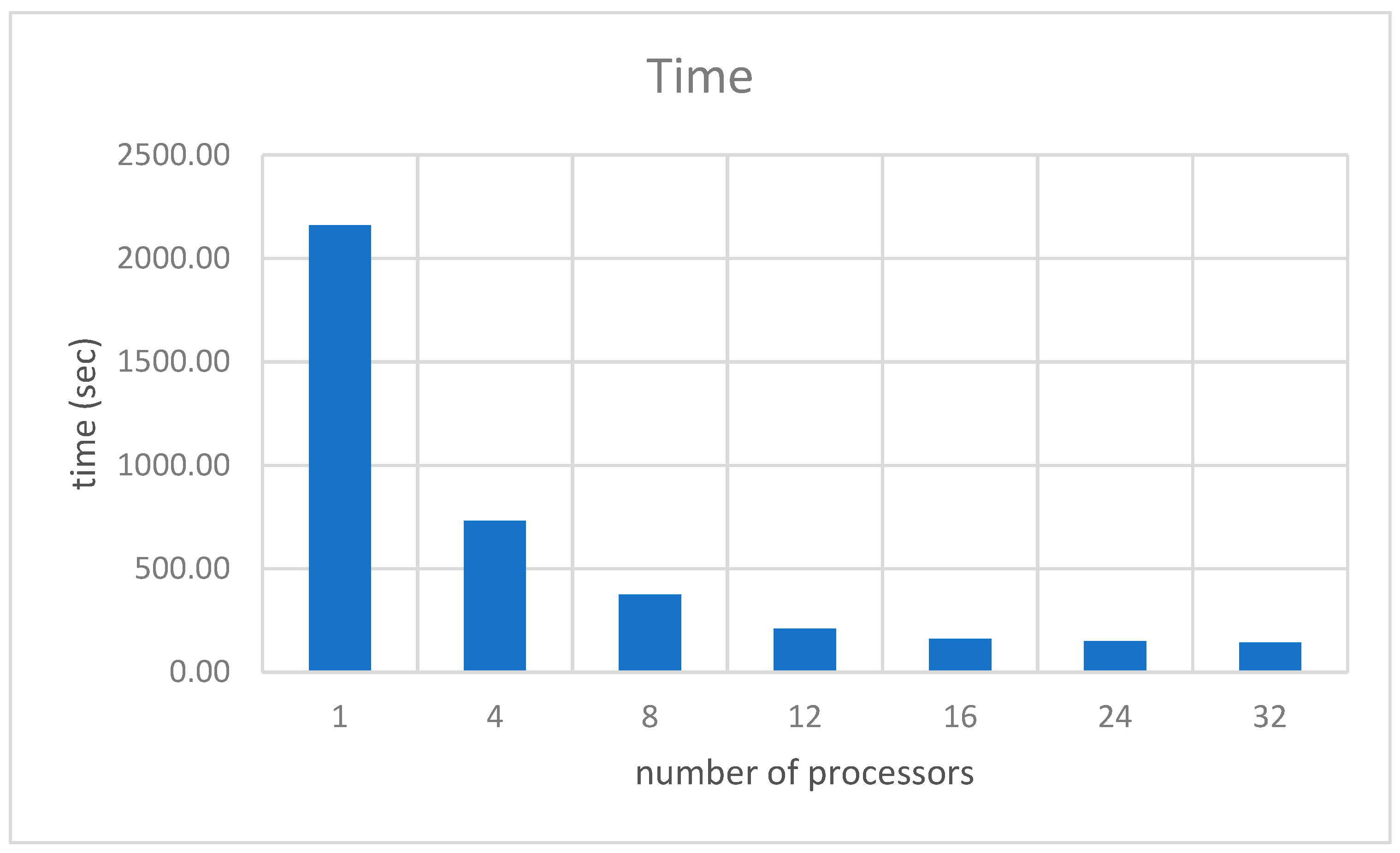
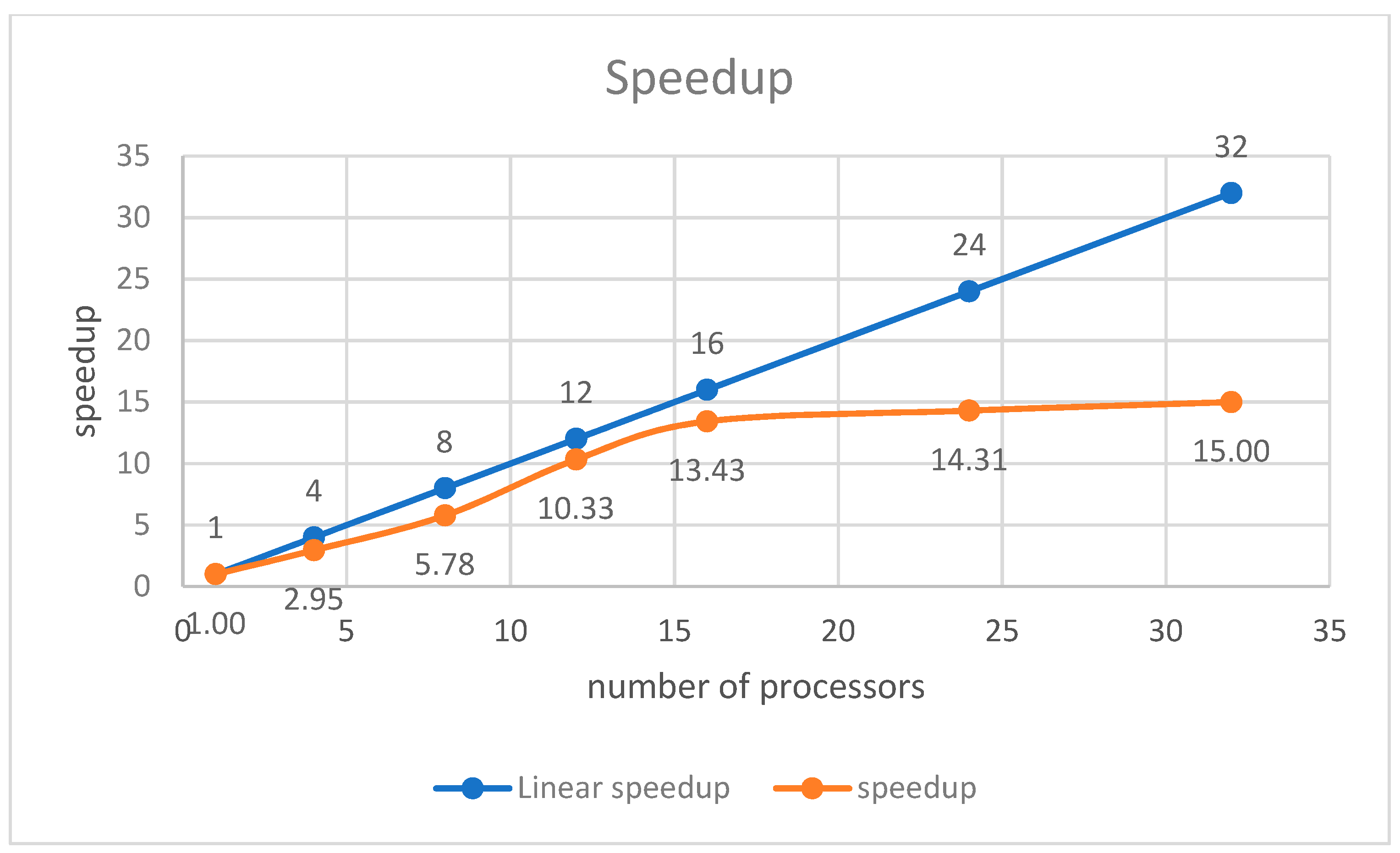
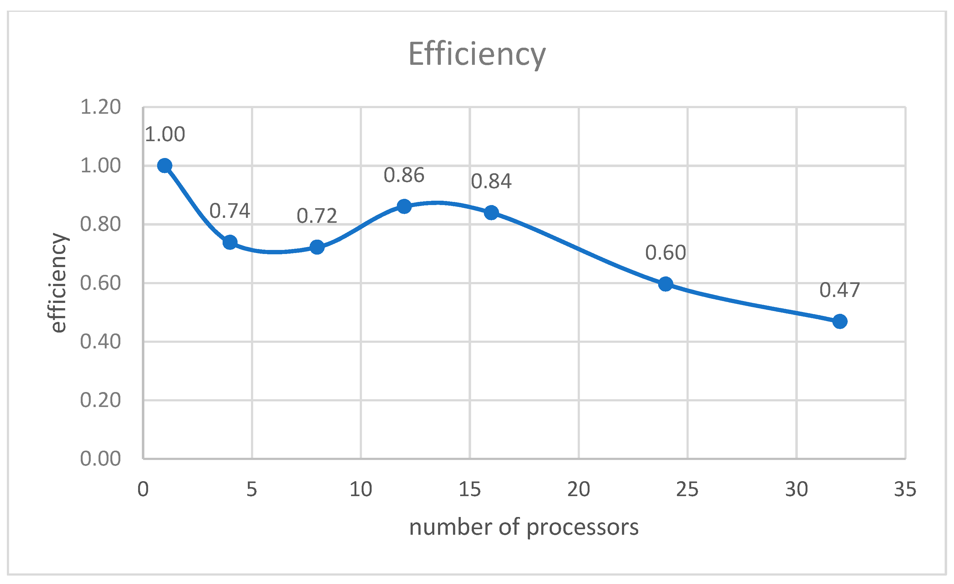
Figure 1. Diagram of solution time/number of processors.
Computation 10 00113 g001
Figure 2. Speedup diagram.
Computation 10 00113 g002
Figure 3. Efficiency diagram.
Computation 10 00113 g003
Figure 4. Placement of 100 circles for the sequential solution, r u p = 257.35311 .
Computation 10 00113 g004
Figure 5. Placement of 100 circles for the parallel solution, r u p = 257.1951 .
Computation 10 00113 g005
Figure 6. Locally optimal layouts of circles in DCBP: (a) n = 50, r * = 182.6996, CPU 1355.85 s for 100 runs; (b) n = 150, r * = 368.4018, CPU 45,910.3 s for 50 runs; (c) n = 300, r * = 520.5562, CPU 24,185.24 s for 50 runs.
Computation 10 00113 g006
Figure 7. Locally optimal arrangement of circles in SCBP: (a) n = 50, d * = 2.05510, CPU 1201.32 s for 100 runs; (b) n = 100, d * = 2.04864, CPU 8090.16 s for 100 runs; (c) n = 150, d * = 2.05183, CPU 19,571.66 s for 100 runs, CPU 8090.16 s for 100 runs.
Computation 10 00113 g007
Table 1. Solution time, speedup and efficiency for a DCBP problem instance with 50 circles solved on the cluster SKIT-4.
ktkCkEk
12159.681.001.00
4731.082.950.74
8373.855.780.72
12209.0410.330.86
16160.7913.430.84
24150.9314.310.60
32144.0215.000.47
Table 2. Coordinates of the placement of 100 circles for the sequential solution, r u p = 257.35311 .
i x i u p y i u p i x i u p y i u p i x i u p y i u p
1139.4106−148.720335−192.0113152.741169−57.0781139.3253
2165.9300−180.735636−20.282057.62837065.7095−121.7164
3−10.4564139.366837−33.4277−76.256371−60.8956205.8394
490.6188−228.005238−25.6351−26.402972−66.4087−215.3460
5−85.8170−120.550939153.564988.77277395.7131204.0172
673.5905127.77104014.8656116.241174−174.886352.7062
7−157.6668127.7678415.8499−16.75817531.2989−218.4935
8−177.5573169.32674265.947343.622076−23.650799.4930
9−70.5784−169.397443−25.8560167.417777−224.790415.9151
1095.745655.28664450.5852229.852678−81.311812.9985
11−109.328144.917845175.1576157.197079−170.0251−13.1497
12150.5197110.560946125.654643.908880219.216552.2319
13−74.5636166.125647178.0610−69.802781−16.3268−178.7973
14−171.4504144.914748−29.88285.314082−196.1507110.9455
15−15.5382−136.804749137.0313139.579283−62.7066−46.1440
16171.818216.293450−18.1262−234.65418414.758534.4732
17−39.7282242.115351−53.789857.118185−1.2195225.3498
18141.1580−200.680352−47.5357−137.203986111.898594.0562
19−158.900091.544853187.9781−110.61518749.906193.0860
20201.8791−139.43815434.1020−166.111388−194.0441−70.3082
2137.9330−105.827255165.984659.281189192.4508108.1568
22−28.672337.29115696.9196152.031290−183.1233−131.3388
23−235.9375−67.31755715.3707−128.51959195.2733−176.2139
24−132.935254.730958171.4069−149.207892−122.5708−170.2925
2593.602127.521859−62.9718−98.143493214.4583−19.6107
26146.8699−169.748860218.3642−81.620494132.4803−17.7144
2711.389876.337961−225.342067.912295−101.784296.3677
2834.5368−2.57846273.82242.36709653.6401−56.2562
29154.235229.516163144.4278185.827197−123.5010−84.7191
30−224.2984−99.440364−8.4552−56.246898−125.8419174.7592
3169.8306−235.205965−232.6625−35.485699123.4839−99.2194
32−174.5260−172.449566−132.392122.735510036.0347163.7371
335.5154−85.036167−118.9449−22.8867
34−79.2399−141.544768−19.4571−105.0456
Table 3. Coordinates of the placement of 100 circles for the parallel solution, r u p = 257.1951 .
i x i u p y i u p i x i u p y i u p i x i u p y i u p
1−45.4108106.959635122.9228−7.10566984.742674.1280
270.2790−41.627736−80.7209−121.059770127.1753−38.8218
382.4623106.046637−75.589378.13917113.1500149.8033
452.482082.934838185.211959.839672−224.0971−22.2112
595.4186−34.883639−65.320397.599273−138.314165.5081
655.495961.142240−27.8345158.983174−35.0326−222.4535
7−10.649672.861641−110.2915−108.829675−98.0049202.3002
8−37.8368−20.61034221.151876.421676−8.7590−155.9050
9−135.0830−88.596443−12.8746104.784277−77.057436.1647
10−52.8890−4.565544−81.7715−18.34247828.2801−41.9345
11−95.1176−137.694945154.9222−7.292379−68.9963−170.5838
1237.291148.789646230.5373−45.383980−68.5395−74.5900
13−151.8092−16.017247114.3888103.878981206.22851.1733
14123.9678−111.075248−97.9383105.109382−149.7678168.1739
15−29.3590132.211649−176.2423−42.556383122.4704180.7840
16−167.0885−73.21915086.9860137.738384−124.5224−47.9457
17−190.43862.910651−23.2266−49.080385−68.3349147.8602
18115.1268−131.220652−11.5071−103.289686−209.5402−82.4969
19−109.4713156.333453−194.4786−132.267987−189.9519120.9591
20101.1534−78.399954218.337887.437788177.8639−53.9579
2120.2577108.409155−42.572375.084989133.262755.4251
22−54.4610−35.01995631.4821−93.84019051.6126−141.7886
23176.970439.44165769.5126−73.61859174.929112.9096
2414.9748−121.25385851.7187114.925792−140.5877−162.9234
25130.605613.509359230.408347.20959355.7506207.8480
26198.756342.503360−157.351617.118394171.4856128.0440
2796.7626−56.842561−97.7063−213.939795173.2629−127.6280
28−110.8739134.378262133.0906−80.403296−26.5284210.9667
29161.219924.08196392.0306−109.071997112.9423−183.1747
30244.497918.478064−138.0666117.507598−208.939951.5080
3155.0646146.750365−48.7620−122.68219936.2227−212.1246
320.9221−73.802166218.9989−85.7685100−6.669421.0142
33−97.009973.122867−162.6154−104.9049
34−173.1583−10.705368−117.59003.5901
Publisher’s Note: MDPI stays neutral with regard to jurisdictional claims in published maps and institutional affiliations.

