Article

Stability Evaluations of Unlined Horseshoe Tunnels Based on Extreme Learning Neural Network

by
Thira Jearsiripongkul
1,
Suraparb Keawsawasvong
2,
Rungkhun Banyong
2,
Sorawit Seehavong
2,
Kongtawan Sangjinda
2,
Chanachai Thongchom
2,
Jitesh T. Chavda
3 and
Chayut Ngamkhanong
4,*
1
Department of Mechanical Engineering, Thammasat School of Engineering, Thammasat University, Pathumthani 12120, Thailand
2
Department of Civil Engineering, Thammasat School of Engineering, Thammasat University, Pathumthani 12120, Thailand
3
Department of Civil Engineering, Sardar Vallabhbhai National Institute of Technology, Surat 395007, India
4
Department of Civil Engineering, Faculty of Engineering, Chulalongkorn University, Bangkok 10330, Thailand
*
Author to whom correspondence should be addressed.
Computation 2022, 10(6), 81; https://doi.org/10.3390/computation10060081
Submission received: 10 April 2022 / Revised: 18 May 2022 / Accepted: 20 May 2022 / Published: 24 May 2022
(This article belongs to the Special Issue Numerical Methods in Geotechnical Engineering)

Abstract

:
This paper presents an Artificial Neural Network (ANN)-based approach for predicting tunnel stability that is both dependable and accurate. Numerical solutions to the instability of unlined horseshoe tunnels in cohesive-frictional soils are established, primarily by employing numerical upper bound (UB) and lower bound (LB) finite element limit analysis (FELA). The training dataset for an ANN model is made up of these numerical solutions. Four dimensionless parameters are required in the parametric analyses, namely the dimensionless overburden factor γD/c′, the cover-depth ratio C/D, the width-depth ratio B/D, and the soil friction angle ϕ. The influence of these dimensionless parameters on the stability factor is explored and illustrated in terms of a design chart. Moreover, the failure mechanisms of a shallow horseshoe tunnel in cohesive-frictional soil that is influenced by the four dimensionless parameters are also provided. Therefore, the current stability solution, based on FELA and ANN models, is presented in this paper, allowing for the efficient and accurate establishment and evaluation of an optimum surcharge loading of shallow horseshoe tunnels in practice.

1. Introduction

The major goal during the construction phase of urban areas is to minimize the destruction of adjacent structures and roadways above the ground surface due to the ground settlement [1,2,3]. For this reason, geotechnical engineers are increasingly concerned with the stability of subsurface structures such as tunnels, underground spaces, abandoned mine workings, and pipelines. The most influential factor regarding shallow h tunnel construction is a lack of stability, which is mostly caused by a surcharge loading above the ground [4,5,6,7,8,9,10,11]. In this study, an artificial neural network (ANN) technique is introduced to solve the tunnel stability problem in the form of a black-box-type prediction model which aims to determine the critical surcharge loading imposed on the ground surface above a shallow elliptical tunnel in cohesive-frictional soil.
The finite element limit analysis (FELA), a sophisticated numerical approach for determining factors of safety and ultimate loads, has recently become an extensive tool for developing precise plastic solutions to tunnel stability problems. To numerically determine genuine plastic collapse loads, this approach employs optimization and finite element discretization techniques by including upper bound (UB) and lower bound (LB) bracketing, which are based on plastic bound theorems to obtain the exact solutions. It is worth noting that the UB and LB approaches are based on either kinematics or equilibrium [12,13]. Sloan [14] provides further information on the features and evolution of UB and LB FELA. Moreover, various researchers, including Sloan and Assadi [15], Wilson et al. [16,17,18], Yamamoto et al. [19,20], Keawsawasvong and Ukritchon [21,22], Keawsawasvong and Likitlersuang [23], Keawsawasvong and Shiau [24], Ukritchon and Keawsawasvong [25,26], Yang et al. [27,28,29], Zhang et al. [30], and Dutta and Bhattacharya [31], have previously performed FELA to overcome the problems of unlined tunnels and trapdoors. In addition, the influence of the non-associated flow rule on the face stability of tunnels was investigated by Di et al. [32] and Zhang et al. [33]. The experimental investigation of mechanical characteristics for linings of twin tunnels was also carried out by Zheng et al. [34]. Note that these investigations were carried out with the constrained shapes of circular, square, rectangular, and elliptical tunnels.
The pain point for maintaining the stability of an underground tunnel is the minimum support pressure. Horseshoe-shaped tunnels can be utilized to minimize the amount of support pressure required and to increase the amount of useable area for openings. To minimize the excavation volume and satisfy the requirements of the geometrical constraints for the construction of roads and related walkways, horseshoe-shaped tunnels are requested. Various past constructions of horseshoe-shaped tunnels can be found in [35,36,37]. A few earlier studies on the stability of horseshoe tunnels are relevant to the present study. The initial study of horseshoe tunnels was carried out by Wilson et al. [18]; the analyses were only conducted in undrained clay, and they provided a comparison with square and rectangular tunnels, indicating that the horseshoe tunnel necessitates a lower support pressure under the same conditions. Subsequently, the stability of dual horseshoe tunnels in cohesive-frictional soil was investigated by Zhang et al. [38]. They employed upper bound analysis to determine the critical unit weight. Later on, Bhattacharya and Sriharsha [39] explored the stability of a long horseshoe tunnel in cohesive-frictional soil under plane strain conditions. The internal support pressure was obtained via lower bound limit analysis. Furthermore, the results were provided in terms of design charts, as were most of the earlier horseshoe tunnel stability solutions. Therefore, it is complicated to apply their results since there are no exact solutions provided, and approximation or interpolation is required to obtain the stability solution.
In this study, the numerical solutions regarding the stability of horseshoe tunnels in cohesive-frictional soils (or sandy soils) under plane strain conditions are presented by employing the numerical technique of FELA to derive UB and LB solutions. In FELA, four dimensionless parameters, namely soil strength parameters, soil unit weight ratio, width-depth ratio, and cover-depth ratio, are utilized to perform a parametric analysis to demonstrate their influence. The relationship between the parameters under consideration is provided, as well as the failure mechanisms. An artificial neural network (ANN) technique, which is one of the soft computing approaches, is used to construct a black-box-type prediction model. This artificial intelligence technique may acquire data from a sufficiently compact information gathering and then establish a black-box-type prediction model to resolve the problems represented by a closed-form equation. This study established an improved model for promptly and reliably evaluating the stability of horseshoe tunnels in cohesive-frictional soils via the combination of ANN and FELA techniques. It should be emphasized that earlier investigations that combined the ANN and FELA techniques were fairly restricted. Only a few investigations by Li et al. [40,41] and Qian [42], which adopted the ANN technique for soil slope stability predictions based on FELA solutions, have been reported. Keawsawasvong et al. [43] later employed a similar method to construct an ANN model for rock tunnel stability problems, employing FELA solutions in conjunction with the HB model as an input data set. Nevertheless, none of the preceding studies have determined an ANN model for horseshoe tunnel stability. Therefore, this study introduces novel soft computing techniques for assessing the stability of horseshoe tunnels in cohesive-frictional soils, resulting in a practical tool that relies on the ANN and FELA methodologies. The concept proposed in this study will allow for the rapid evaluation of these concerns in practice for shallow tunnel designs and construction in metropolitan regions.

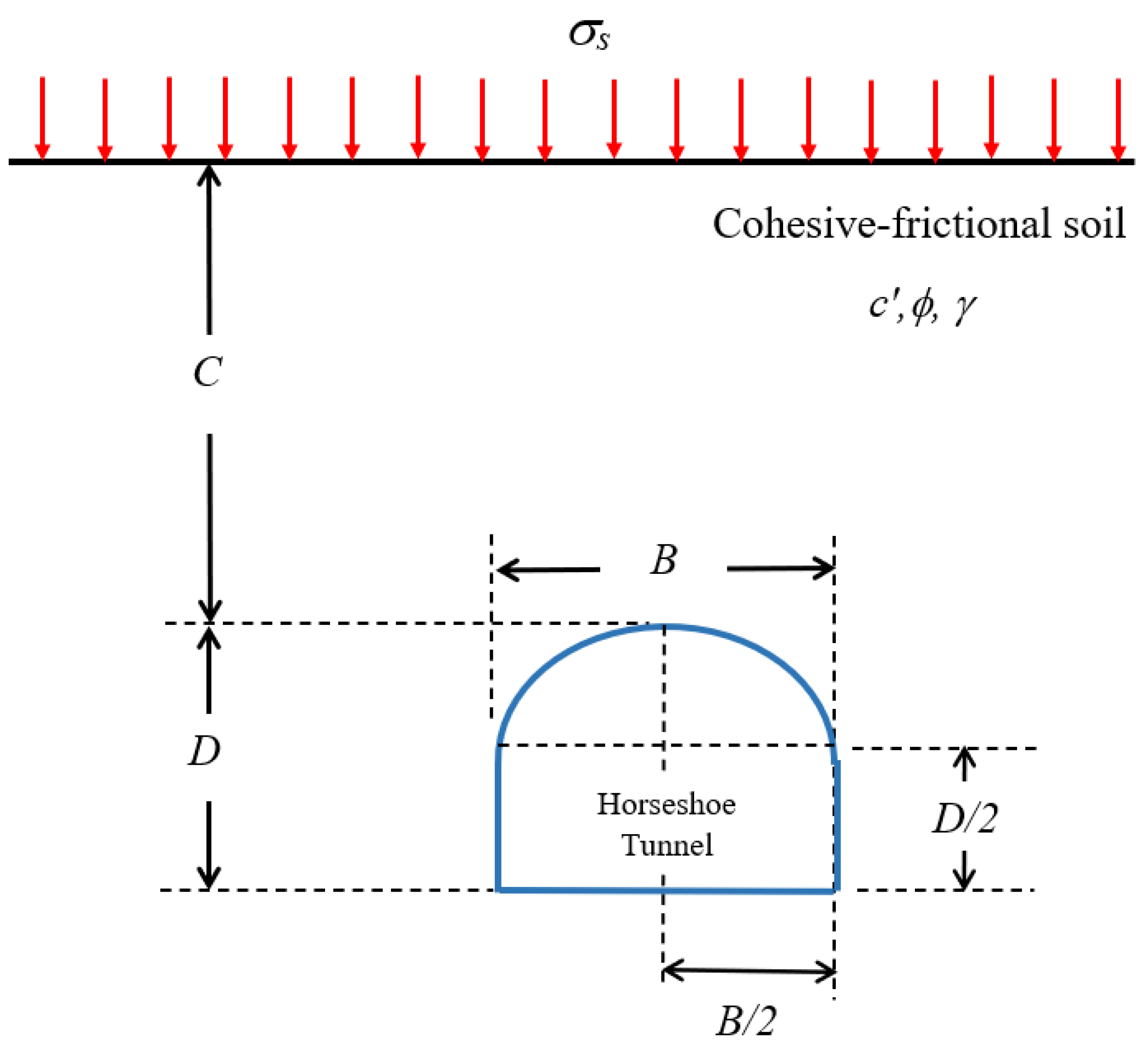
2. Problem Statement

Figure 1 shows the problem definition of an unsupported infinitely long horseshoe tunnel in cohesive-frictional soil under plane strain conditions. The geometry of the tunnel consists of two parts, which are the half-circular tunnel roof with a diameter B and the rectangular section with a width B and a vertical height of D/2. The tunnel has an overall height of D, which is located beneath the ground level with a cover depth C. With the accompanying flow rule, the soil mass around the tunnel is assumed to obey the Mohr-Coulomb yield criterion. According to the Mohr-Coulomb yield criterion, the soil profile is controlled by three parameters: effective cohesion (c′), effective friction angle (ϕ), and unit weight (γ). The ground surface is subjected to a vertical surcharge loading (σs). It is worth noting that the soil unit weight and the surface surcharge operate as vertical driving forces leading to the event of a collapse, while the effective cohesion operates as an uplift force that resists the driving force.
To simplify the analyzed parameters, a dimensionless technique Butterfield [44] was adopted with six considered dimensional input parameters, namely C, D, B, γ, c′, and ϕ, which mainly influence the outcome of critical surcharge loading (σs) at the surface of the ground. Moreover, the six dimensional input parameters are reduced into four dimensionless input parameters, which can be stated in terms of the stability factor of horseshoe tunnels in cohesive-frictional soil as follows:
σ s c = f ( γ D c , C D , B D , ϕ )
where σs/c′ represents the stability factor of horseshoe tunnel;
γD/c′ represents the dimensionless overburden factor;
C/D represents the cover-depth ratio;
B/D represents the width-depth ratio;
ϕ represents the soil friction angle.
The parametric analysis for the considered parameters provides a variety of alternatives that are useful in practice. More details on the chosen range of the four dimensionless parameters encompassed in this study are provided in Table 1. The dimensionless input and output data examined by FELA, on the other hand, are critical for developing a nonlinear input–output mapping of the problem of horseshoe tunnel instability in cohesive-frictional soils, which applies a neural network trained throughout an extreme learning neural network.

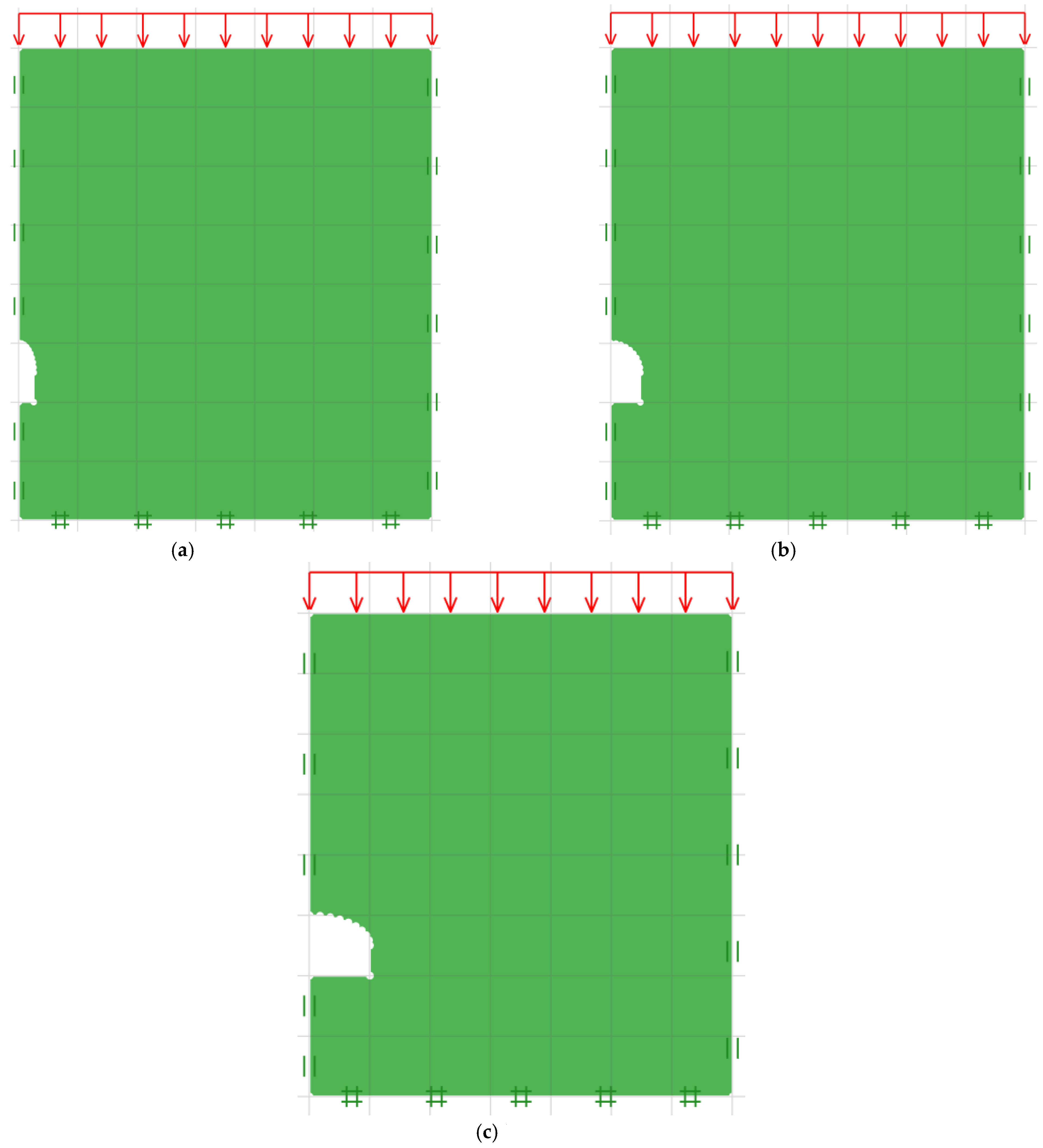
3. Method of Analysis

The present study employs the numerical program OptumG2 FELA [45] to analyze the stability problems of a horseshoe tunnel in cohesive-frictional soil. The numerical results obtained by FELA will be utilized as input data in the ANN model. Numerous geotechnical engineering concerns have been solved entirely by applying FELA to evaluate the stability solution in terms of safety factors and limit loads (e.g., [46,47,48,49,50,51,52,53,54,55,56,57,58]). A depth ratio of C/D = 4 and varied values of B/D = 0.5, 1, and 2 are the selected cases of the models developed by OptumG2, as seen in Figure 2a–c. Only half of the domain of the horseshoe tunnel was simulated, with the line of symmetry placed to the domain’s left boundary which is also represented in Figure 2a–c. In the FELA analysis, all numerical models are subjected to the standard boundary conditions, where the left and right boundaries are considered to be roller support that only allows the movement in the vertical direction. The bottom boundary is considered to be a fixed support in which no movement is allowed in both the horizontal and vertical directions along the plane. Free surfaces are provided within the horseshoe tunnel and on the ground surface to indicate that free movement is permitted. Furthermore, the loading multiplier function in OptumG2 is employed to place a uniform surcharge vertically across the top of the ground surface. The critical surcharge loading (σs) in the event of collapse is optimized according to the UB and the LB FELA.
In both the LB and the UB FELA, the soils are discretized into a series of triangular components that are dispersed throughout the domain of the horseshoe tunnel problems. The LB solutions are obtained in the LB FELA analysis by establishing a statically acceptable stress field, located inside three-noded triangle elements, that has its own fundamental unknowns of stress components. Through the loading multiplier approach, the collapse surcharge is maximized by obeying all equilibrium requirements based on the LB FELA technique that is developed throughout the whole domain of the problem. Moreover, a kinematically acceptable velocity field in the domain is generated in the UB FELA analysis, using each node’s vertical and horizontal velocities as the fundamental unknowns. The loading multiplier approach is used to reduce the collapse surcharge by comparing the level of current activity performed by the external pressure with the total internal power dissipation. The domain sizes are selected to be broad enough to include the plastic shear zone in all simulations of the LB and UB FELA models. The overlapping of the plastic shear zone at the right or bottom boundary should not be observed, since this would affect the correctness of the solution. Thus, the sizes of the right and bottom boundaries are set to be 7D and 2D, respectively, which are sufficient to avoid the effect of insufficient boundaries (see Figure 2).
In order to provide better precise limit solutions, the significant function of mesh adaptivity in OptumG2 is enabled in all UB and LB simulations. An autonomously adaptable mesh refinement was used to achieve the tight UB and LB solutions. Furthermore, the effective approach of automatic mesh adaptivity with shear dissipation optimization ensures that the generated LB and UB solutions are more accurate. With a starting mesh amount of 5000 elements that will be raised to the final mesh amount of 10,000 elements, this study applies five adaptive meshing phases. The finalized adaptive meshes may be utilized to display the horseshoe tunnel’s failure processes in cohesive-frictional soil. Ciria et al. [59] have written a paper that goes into further detail about this mesh adaptivity characteristic.

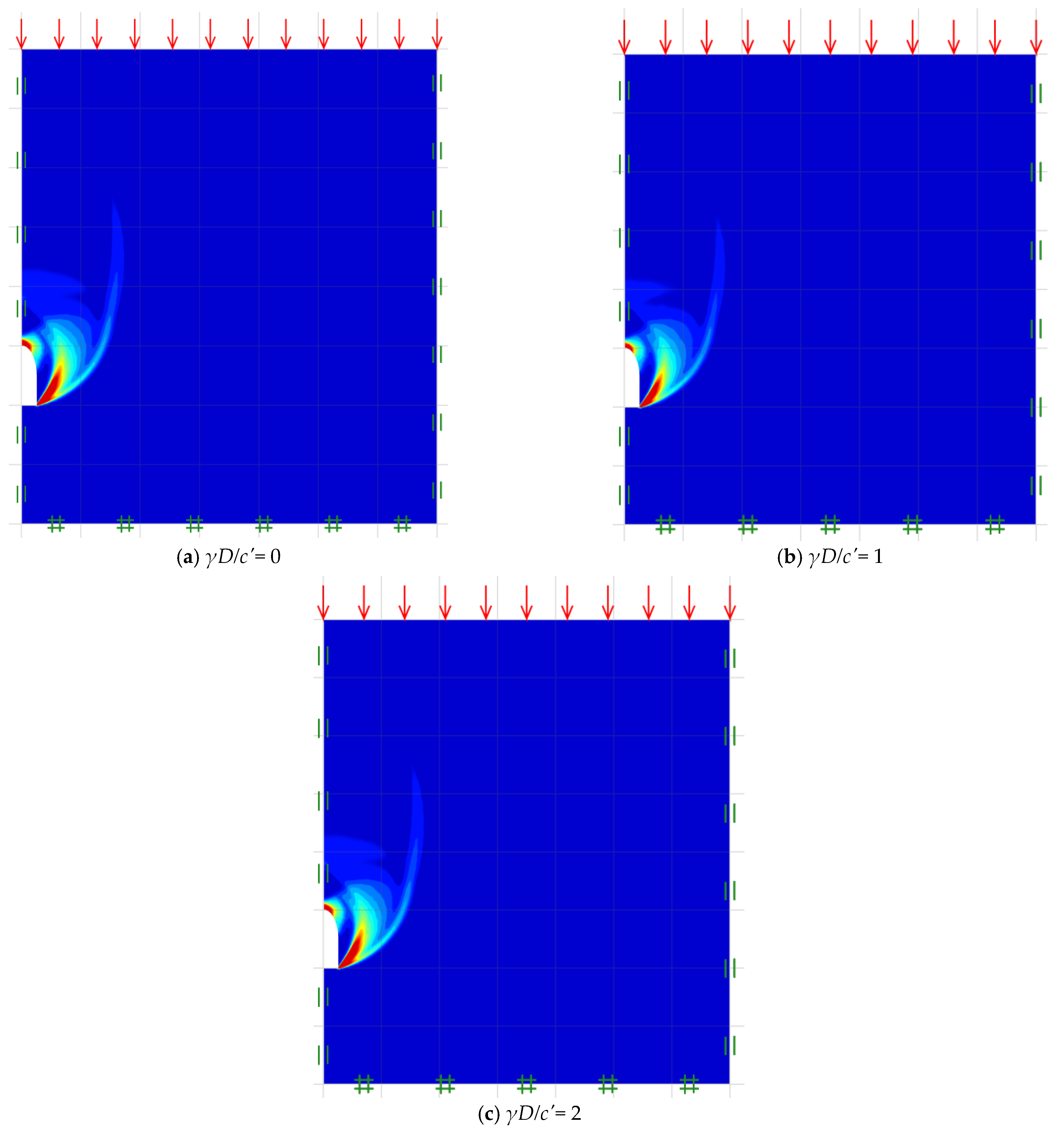
4. Results and Discussion

Since the differences between the current UB and LB solutions are very small (less than 1%), the average (Ave) solutions computed from the average values of the UB and LB FELA solutions, which can be considered as rigorous solutions, are presented in this study. Note that only the solutions of the active collapse of tunnels are considered in this study. Figure 3, Figure 4, Figure 5 and Figure 6 and Table 2 demonstrate the average solution of the stability factor of a horseshoe tunnel in cohesive-frictional soil. Table 2 contains the results data that will eventually be utilized as input data in the ANN technique, which will be described in the next section. Note that the sign conventions for the dimensionless load factors presented in Table 2 show that a positive sign corresponds to the cases where the ground above the tunnel can support the compressive normal stress and the self-weight of soil masses. In contrast, a negative sign corresponds to the cases where only the tensile normal stress can apply on the ground surface. The later cases of the negative sign rarely happen in practice since compressive normal stress is mostly applied on the ground surface. Nevertheless, these cases can indicate that if there is no tensile normal stress applied on the ground surface, the soils around the tunnel will certainly collapse due to the driving force from the self-weight of soil masses.
Throughout all numerical results, Figure 3a,b represents the influence of the soil friction angle on the stability factor in the selected cases of γD/c′ = 0 and C/D = 1 and 4, respectively, with various values of B/D = 0.5, 0.75, 1, 1.333, and 2. A non-linear increasing relationship between ϕ on σs/c′ is discovered, in other words as the soil frictional angle increases, the strength of soil around the tunnel also increases. The influences of the overburden factor γD/c′ on the stability number σs/c′ with the selected cases of C/D = 0 and ϕ = 0° and 5 are shown in Figure 4a,b, respectively. A decreasing linear relationship is found, with an increase in γD/c′ leading to a decrease in σs/c′. Figure 5a,b demonstrates the trend of the cover-depth ratio C/D on the stability factor σs/c′ for ϕ = 25° and γD/c′ = 0 and 1, respectively. A nonlinear rising relationship is observed, with an increase in C/D resulting in an increase in σs/c′. Moreover, the influence of the width-depth ratio B/D on the stability factors σs/c′ of horseshoe tunnels with ϕ = 25° and γD/c′ = 0 and 1 is investigated and displayed in Figure 6a,b. The charts include four distinct values of C/D = 1, 2, 3, and 4. It is discovered that a nonlinear decreasing relationship occurs, implying that higher B/D values result in a lower stability factor σs/c′.
The adaptive meshes concept is finally utilized to monitor the failure mechanisms of unlined horseshoe tunnels in cohesive-frictional soil. Figure 7a–c illustrates samples of final adaptive meshes for the selected values C/D = 5, γD/c′ = 0, and ϕ = 25° with varying values of B/D = 0.5, 1, and 2. More details are described earlier. In addition, the influence of analyzed parameters such as γD/c′, C/D, B/D, and ϕ on the horseshoe tunnel failure mechanisms are explored and demonstrated in Figure 8, Figure 9, Figure 10, Figure 11 and Figure 12. The illustrated failure mechanisms are related to the shear dissipations of unlined horseshoe tunnels in cohesive-frictional soil. Figure 8a–c, for varied values of B/D = 0.5, 1, and 2, clearly indicates that the failure zone extent gets larger and higher off the ground surface as the tunnel gets wider (higher B/D). In Figure 9a–d and Figure 10a–d, it seems like the soil frictional angle of the overburden factor does not have much influence on the failure mechanisms for the case of the narrow tunnel as well as the overburden factor. Figure 11a–d illustrates the influence of the cover-depth ratio on the failure mechanisms. The failure zone appears to extend in both vertical and horizontal planes as the tunnel is placed deeper (higher C/D). Thus, the deeper the tunnel, the greater the failure zone. In all figures, the type of failure mechanism of the horseshoe tunnel is mostly unchanged, resembling a half-spiral opening failure.
The current average FELA solutions of an unlined horseshoe tunnel are compared to prior investigation to validate the stability factor obtained from this solution. The comparison was made up in terms of stability numbers from the present solution to those reported by Yamamoto et al. [19,20], as shown in Figure 12. It should be noted that the solutions given by Yamamoto et al. [19,20] are restricted to circular and square tunnels with B/D = 1. The soil unit weight is set to zero in comparison to eliminate the overburden factor. Therefore, the current results are equivalent to those in Yamamoto et al. [19,20], demonstrating that the developed FELA solution is exceptionally exact and trustworthy in practice.

5. Proposed Predictive Models

5.1. Multiple Linear Regression

Linear regression is the simplest method to construct a linear relationship between scalar responses (output known as dependent variables) and explanatory variables (input known as independent variables). In this study, four independent variables are considered; therefore, the process is called “multiple linear regression”.
As indicated in Equation (2), the output is a dependent variable that may be determined from the combination of the input or independent variables.
y i = β 0 + β 1 x i 1 + β 2 x i 2 + + β p x i p + ϵ  
where
y i = dependent variable (output);
x i 1 ,   x i 2 ,     x i p = independent variables (input);
β 0 = y-intercept (constant term);
β 1 ,   β 1 , ,   β p = slope coefficients for each explanatory variable;
ϵ = the model’s error term (also known as the residuals).

5.2. Artificial Neural Network (ANN)

An Artificial Neural Network (ANN) is a data prediction framework based on existing features created from the human mind structure. In order to handle complicated information, it mimics the neural system’s processing method in the human brain. With many nodes (or neurons) wired together, a neural network is a computer model that may be used for many different purposes.
ANN comprises three layers: an input layer, a hidden layer, and an output layer, as shown in Figure 13. In this study, the input layer consists of four nodes representing C/D, B/D, γD/c′, and ϕ. The second layer is the hidden layer, consisting of one or more threshold logic unit layers. Generally, the number of hidden layers and hidden neurons is chosen via the trial-and-error method. It is generally recommended to start from one hidden layer. The number of hidden neurons is varied from one to the number that can create the proper model with high accuracy. This layer aims to convert the information into content that the output layer can use to predict the data. It is within this layer that the weighted sums of the inputs are calculated and a step function is applied to them before they are sent off as an output through the use of the rectified linear unit (ReLU) activation function, which provides nonlinearity in the network. The final layer is the output layer presenting the dependent variables. In this paper, the output layer consists of one node, which is a predicted stability factor of shallow elliptical tunnels in cohesive-frictional soils.

5.3. Cross-Validation and Performance Measures

In this study, the stratified tenfold cross-validation is used due to the limited number of datasets. This method can replicate the drawback of the splitting method into training and testing datasets when the datasets are limited.
The proposed cross-validation method randomly divides the datasets into ten sections, with the classes represented in about the same proportions as in the entire dataset. Before assessing the error rate on the holdout set, each section is performed in turn, and the remaining nine-tenths are later tested. As a result, the learning operation is repeated ten times on different training sets. After that, these errors are averages to employ the representative of the error estimation. However, it is highly recommended to repeat the cross-validation process 10 times, since a single tenfold cross-validation is not reliable. This leads to the learning algorithm being repeated 100 times on datasets that are all nine-tenths the size of the original.
In this paper, three well-known statistical performance measures of the obtained models are the coefficient of determination (R-squared, R2), Root Mean Squared Error (RMSE), and Mean Absolute Error (MAE). It should be noted that the high accuracy prediction model leads to a high value of the coefficient of determination, whereas RMSE and MAE calculate errors instead of accuracy, so the good performance of the prediction model is indicated by lower values. These statistical performance measures are used to compare the performance of the models.

5.4. Predictive Equations

5.4.1. Multiple Linear Regression

A multiple linear regression model is first obtained consisting of the weight of each parameter. The coefficients are evaluated in WEKA software. The multiple linear regression equation is shown in Equation (3).
y = 11.1882 x 1 + 1.3637 x 2 5.4693 x 3 + 6.2233 x 4 5.7233
where y represents the stability factor σs/c′ whereas x 1 , x 2 , x 3   and   x 4 are the dimensionless input parameters namely, B/D, ϕ, γD/c′, and C/D respectively. The statistical values: R2, MAE and RMSE are 0.6616, 11.8803, and 19.0166, respectively (see Table 3).

5.4.2. Artificial Neural Network

In this study, the number of ANN modes is developed considering different numbers of neurons in the hidden layer. The performance of the models against the number of hidden neurons is plotted in Figure 14. It can be seen that after reaching a certain number of neurons, the performance of ANN models is likely to stabilize. In this study, ANN with the architecture of 4-7-1 is selected to be the best ANN model, as it shows the highest accuracy and the lowest errors compared to other models. Figure 15 compares the results obtained by the FELA solution and the ANN model. It is found that the predicted values from ANN are in agreement with those from the FELA solution. Table 3 also compares the performances of the MLR and ANN models. It is clear that the ANN model performs much better than the MLR model.
Figure 16 presents the multilayer network with the dimensions of input, weight, bias, and the output matrices of the proposed ANN model for stability evaluation of shallow horseshoe tunnels. From Figure 16, IW1 and IW2 represent the hidden weight matrix and output weight matrix, respectively, and b1 and b2 represent the bias matrices in the hidden and output layers.
Predictive Equation (4) can be developed based on tansig function, weight and bias from ANN model.
P r e d i c t e d   v a l u e = [ i = 1 N I W 2 i t a n s i g ( j = 1 J I W 1 i j x j + b 1 i ) + b 2 ]
where N is the number of hidden neurons; X is the independent parameters (input); J is the number of independent parameters. (b1i). Table 4 presents the neural network constants of the optimal ANN model, including weight matrix and bias for the stability factor calculation of shallow elliptical tunnels in cohesive-frictional soils. The values obtained from the optimal ANN networks can be used to develop predictive equation functions and test new datasets with different variations of parameters within the required ranges.

6. Conclusions

The study aims to establish a machine learning-aided prediction of the stability of shallow elliptical tunnels in cohesive-frictional soils. The four input dimensionless parameters include the dimensionless overburden factor γD/c′, the cover-depth ratio C/D, the width-depth ratio B/D, and the soil friction angle ϕ. The influences of all input dimensionless parameters on the solutions of the stability factor σs/c′ are investigated. The solutions are computed using the finite element limit analysis (FELA). An Artificial Neural Network (ANN) model is then developed based on the training data of FELA solutions. Since it is time-consuming to develop the algorithm of the FELA and use the FELA software to obtain the stability solutions of elliptical tunnels in sands on a case-by-case basis, a proposed scheme of the ANN model is developed in this study. In addition, proper software is not usually user-friendly, and additional resources capable of providing information that is useful for decision-making are required. The combination of FELA solutions and the ANN is then presented as a guide for geotechnical engineers. Note that the optimal machine learning models for predicting the stability factor of this problem can be evaluated based on some matrices. It is notable that only one hidden layer is sufficient to create a high-performance neural network model, as R2 is already high and MSE is extremely low, showing that the optimal model is reliable and can be used to accurately predict the stability factor. Finally, the obtained trained networks can be further used to test new data for predicting the stability factor of shallow elliptical tunnels in cohesive-frictional soils using the weight matrix and bias derived in this study.

Author Contributions

Conceptualization, T.J., S.K. and C.N.; methodology, T.J., S.K. and C.N.; software, R.B., S.S., K.S., C.T. and J.T.C.; validation, R.B., S.S., K.S., C.T. and J.T.C.; formal analysis, T.J., S.K., R.B., S.S., K.S., C.T., J.T.C. and C.N.; investigation, T.J., S.K., R.B., S.S., K.S., C.T., J.T.C. and C.N.; data curation, R.B., S.S., K.S., C.T. and J.T.C.; writing—original draft preparation, T.J., S.K., R.B. and C.N.; writing—review and editing, T.J., S.K., R.B. and C.N.; visualization, T.J., S.K., R.B., S.S., K.S., C.T., J.T.C. and C.N.; supervision, T.J., S.K. and C.N.; project administration, T.J., S.K. and C.N.; funding acquisition, T.J., S.K., C.T. and C.N. All authors have read and agreed to the published version of the manuscript.

Funding

This research project was also supported by grants for development of new faculty staff, Ratchadaphiseksomphot Fund, Chulalongkorn University.

Institutional Review Board Statement

Not applicable.

Informed Consent Statement

Not applicable.

Data Availability Statement

The data and materials in this paper are available.

Acknowledgments

This work was supported by Thammasat University Research Unit in Structural and Foundation Engineering.

Conflicts of Interest

The authors declare no conflict of interest.

References

  1. Sloan, S.; Assadi, A. Undrained stability of a plane strain heading. Can. Geotech. J. 1994, 31, 443–450. [Google Scholar] [CrossRef]
  2. Ukritchon, B.; Keawsawasvong, S.; Yingchaloenkitkhajorn, K. Undrained face stability of tunnels in Bangkok subsoils. Int. J. Geotech. Eng. 2017, 11, 262–277. [Google Scholar] [CrossRef]
  3. Mair, R.J. Centrifugal Modelling of Tunnel Construction in Soft Clay. Ph.D. Thesis, Cambridge University, Cambridge, UK, 1979. [Google Scholar] [CrossRef]
  4. Shiau, J.; Al-Asadi, F. Three-Dimensional Analysis of Circular Tunnel Headings Using Broms and Bennermark’s Original Stability Number. Int. J. Geomech. 2020, 20, 06020015. [Google Scholar] [CrossRef]
  5. Ukritchon, B.; Keawsawasvong, S. Lower bound stability analysis of plane strain headings in Hoek-Brown rock masses. Tunn. Undergr. Space Technol. 2019, 84, 99–112. [Google Scholar] [CrossRef]
  6. Ukritchon, B.; Keawsawasvong, S. Stability of Retained Soils Behind Underground Walls with an Opening Using Lower Bound Limit Analysis and Second-Order Cone Programming. Geotech. Geol. Eng. 2019, 37, 1609–1625. [Google Scholar] [CrossRef]
  7. Ukritchon, B.; Keawsawasvong, S. Design equations for undrained stability of opening in underground walls. Tunn. Undergr. Space Technol. 2017, 70, 214–220. [Google Scholar] [CrossRef]
  8. Fraldi, M.; Guarracino, F. Limit analysis of collapse mechanisms in cavities and tunnels according to the Hoek–Brown failure criterion. Int. J. Rock Mech. Min. Sci. 2009, 46, 665–673. [Google Scholar] [CrossRef]
  9. Davis, E.H.; Gunn, M.J.; Mair, R.J.; Seneviratine, H.N. The stability of shallow tunnels and underground openings in cohesive material. Geotechnique 1980, 30, 397–416. [Google Scholar] [CrossRef]
  10. Ukritchon, B.; Keawsawasvong, S. Lower bound solutions for undrained face stability of plane strain tunnel headings in anisotropic and non-homogeneous clays. Comput. Geotech. 2019, 112, 204–217. [Google Scholar] [CrossRef]
  11. Ukritchon, B.; Yingchaloenkitkhajorn, K.; Keawsawasvong, S. Three-dimensional undrained tunnel face stability in clay with a linearly increasing shear strength with depth. Comput. Geotech. 2017, 88, 146–151. [Google Scholar] [CrossRef]
  12. Drucker, D.C.; Prager, W.; Greenberg, H.J. Extended limit design theorems for continuous media. Q. Appl. Math. 1952, 9, 381–389. [Google Scholar] [CrossRef] [Green Version]
  13. Chen, W.F.; Liu, X.L. Limit Analysis in Soil Mechanics; Elsevier: Amsterdam, The Netherlands, 1990. [Google Scholar]
  14. Sloan, S. Geotechnical stability analysis. Géotechnique 2013, 63, 531–571. [Google Scholar] [CrossRef] [Green Version]
  15. Sloan, S.W.; Assadi, A. Undrained stability of a square tunnel whose strength increases linearly with depth. Comput. Geotech. 1991, 12, 321–346. [Google Scholar] [CrossRef]
  16. Wilson, D.W.; Abbo, A.J.; Sloan, S.W.; Lyamin, A.V. Undrained stability of a circular tunnel where the shear strength increases linearly with depth. Can. Geotech. J. 2011, 48, 1328–1342. [Google Scholar] [CrossRef]
  17. Abbo, A.J.; Wilson, D.W.; Sloan, S.; Lyamin, A. Undrained stability of wide rectangular tunnels. Comput. Geotech. 2013, 53, 46–59. [Google Scholar] [CrossRef]
  18. Wilson, D.W.; Abbo, A.J.; Sloan, S.W. Undrained stability of tall tunnels. In Proceedings of the 14th International Conference of International Association for Computer Methods and Recent Advances in Geomechanics, Kyoto, Japan, 24 September 2014. [Google Scholar]
  19. Yamamoto, K.; Lyamin, A.; Wilson, D.W.; Sloan, S.; Abbo, A. Stability of a circular tunnel in cohesive-frictional soil subjected to surcharge loading. Comput. Geotech. 2011, 38, 504–514. [Google Scholar] [CrossRef]
  20. Yamamoto, K.; Lyamin, A.; Wilson, D.W.; Sloan, S.; Abbo, A. Stability of a single tunnel in cohesive–frictional soil subjected to surcharge loading. Can. Geotech. J. 2011, 48, 1841–1854. [Google Scholar] [CrossRef]
  21. Keawsawasvong, S.; Ukritchon, B. Undrained stability of plane strain active trapdoors in anisotropic and non-homogeneous clays. Tunn. Undergr. Space Technol. 2021, 107, 103628. [Google Scholar] [CrossRef]
  22. Keawsawasvong, S.; Ukritchon, B. Design equation for stability of shallow unlined circular tunnels in Hoek-Brown rock masses. Bull. Eng. Geol. Environ. 2020, 79, 4167–4190. [Google Scholar] [CrossRef]
  23. Keawsawasvong, S.; Likitlersuang, S. Undrained stability of active trapdoors in two-layered clays. Undergr. Space 2021, 6, 446–454. [Google Scholar] [CrossRef]
  24. Keawsawasvong, S.; Shiau, J. Stability of active trapdoors in axisymmetry. Undergr. Space 2022, 7, 50–57. [Google Scholar] [CrossRef]
  25. Ukritchon, B.; Keawsawasvong, S. Stability of unlined square tunnels in Hoek-Brown rock masses based on lower bound analysis. Comput. Geotech. 2019, 105, 249–264. [Google Scholar] [CrossRef]
  26. Ukritchon, B.; Keawsawasvong, S. Undrained Stability of Unlined Square Tunnels in Clays with Linearly Increasing Anisotropic Shear Strength. Geotech. Geol. Eng. 2020, 38, 897–915. [Google Scholar] [CrossRef]
  27. Yang, F.; Zhang, J.; Yang, J.; Zhao, L.; Zheng, X. Stability analysis of unlined elliptical tunnel using finite element upper-bound method with rigid translatory moving elements. Tunn. Undergr. Space Technol. 2015, 50, 13–22. [Google Scholar] [CrossRef]
  28. Yang, F.; Sun, X.; Zheng, X.; Yang, J. Stability analysis of a deep buried elliptical tunnel in cohesive–frictional (c–ϕ) soils with a nonassociated flow rule. Can. Geotech. J. 2017, 54, 736–741. [Google Scholar] [CrossRef]
  29. Yang, F.; Sun, X.; Zou, J.; Zheng, X. Analysis of an elliptical tunnel affected by surcharge loading. Proc. Inst. Civ. Eng.-Geotech. Eng. 2019, 172, 312–319. [Google Scholar] [CrossRef]
  30. Zhang, J.; Yang, J.; Yang, F.; Zhang, X.; Zheng, X. Upper-Bound Solution for Stability Number of Elliptical Tunnel in Cohesionless Soils. Int. J. Geomech. 2017, 17, 06016011. [Google Scholar] [CrossRef]
  31. Dutta, P.; Bhattacharya, P. Determination of internal pressure for the stability of dual elliptical tunnels in soft clay. Geomech. Geoengin. 2021, 16, 67–79. [Google Scholar] [CrossRef]
  32. Di, Q.; Li, P.; Zhang, M.; Guo, C.; Wang, F.; Wei, Y. Evaluation of Tunnel Face Stability Subjected to Seismic Load Based on the Non-associated Flow Rule. KSCE J. Civ. Eng. 2022, 26, 2478–2489. [Google Scholar] [CrossRef]
  33. Zhang, M.; Di, Q.; Li, P.; Wei, Y.; Wang, F. Influence of non-associated flow rule on face stability for tunnels in cohesive–frictional soils. Tunn. Undergr. Space Technol. 2022, 121, 104320. [Google Scholar] [CrossRef]
  34. Zheng, H.; Li, P.; Ma, G.; Zhang, Q. Experimental investigation of mechanical characteristics for linings of twins tunnels with asymmetric cross-section. Tunn. Undergr. Space Technol. 2022, 119, 104209. [Google Scholar] [CrossRef]
  35. Li, Y.; Zhou, G.; Tang, C.; Wang, S.; Wang, K.; Wang, T. Influence of undercrossing tunnel excavation on the settlement of a metro station in Dalian. Bull. Eng. Geol. Environ. 2021, 80, 4673–4687. [Google Scholar] [CrossRef]
  36. He, Z.; Li, C.; He, Q.; Liu, Y.; Chen, J. Numerical Parametric Study of Countermeasures to Alleviate the Tunnel Excavation Effects on an Existing Tunnel in a Shallow-Buried Environment near a Slope. Appl. Sci. 2020, 10, 608. [Google Scholar] [CrossRef] [Green Version]
  37. Ng, C.W.W.; Wang, R.; Boonyarak, T. A comparative study of the different responses of circular and horseshoe-shaped tunnels to an advancing tunnel underneath. Geotech. Lett. 2016, 6, 168–175. [Google Scholar] [CrossRef]
  38. Zhang, J.; Feng, T.; Yang, J.; Yang, F.; Gao, Y. Upper-bound stability analysis of dual unlined horseshoe-shaped tunnels subjected to gravity. Comput. Geotech. 2018, 97, 103–110. [Google Scholar] [CrossRef]
  39. Bhattacharya, P.; Sriharsha, P. Stability of Horseshoe Tunnel in Cohesive-Frictional Soil. Int. J. Geomech. 2020, 20, 06020021. [Google Scholar] [CrossRef]
  40. Li, A.; Khoo, S.; Lyamin, A.; Wang, Y. Rock slope stability analyses using extreme learning neural network and terminal steepest descent algorithm. Autom. Constr. 2016, 65, 42–50. [Google Scholar] [CrossRef]
  41. Li, A.-J.; Lim, K.; Fatty, A. Stability evaluations of three-layered soil slopes based on extreme learning neural network. J. Chin. Inst. Eng. 2020, 43, 628–637. [Google Scholar] [CrossRef]
  42. Qian, Z.; Li, A.; Chen, W.; Lyamin, A.; Jiang, J. An artificial neural network approach to inhomogeneous soil slope stability predictions based on limit analysis methods. Soils Found. 2019, 59, 556–569. [Google Scholar] [CrossRef]
  43. Keawsawasvong, S.; Seehavong, S.; Ngamkhanong, C. Application of artificial neural networks for predicting the stability of rectangular tunnel in Hoek-Brown rock masses. Front. Built Environ. 2022, 8, 837745. [Google Scholar] [CrossRef]
  44. Butterfield, R. Dimensional analysis for geotechnical engineering. Géotechnique 1999, 49, 357–366. [Google Scholar] [CrossRef]
  45. Krabbenhoft, K.; Lyamin, A.; Krabbenhoft, J. Optum Computational Engineering (OptumG2 Version G2 2020_2020.08.17). Available online: https://www.optumce.com (accessed on 1 July 2020).
  46. Ukritchon, B.; Keawsawasvong, S. Error in Ito and Matsui’s limit equilibrium solution of lateral force on a row of stabilizing piles. J. Geotech. Geoenviron. Eng. 2017, 143, 02817004. [Google Scholar] [CrossRef]
  47. Ukritchon, B.; Keawsawasvong, S. A new design equation for drained stability of conical slopes in cohesive-frictional soils. J. Rock Mech. Geotech. Eng. 2018, 10, 358–366. [Google Scholar] [CrossRef]
  48. Ukritchon, B.; Wongtoythong, P.; Keawsawasvong, S. New design equation for undrained pullout capacity of suction caissons considering combined effects of caisson aspect ratio, adhesion factor at interface, and linearly increasing strength. Appl. Ocean Res. 2018, 75, 1–14. [Google Scholar] [CrossRef]
  49. Ukritchon, B.; Keawsawasvong, S. Design equations of uplift capacity of circular piles in sands. Appl. Ocean. Res. 2019, 90, 101844. [Google Scholar] [CrossRef]
  50. Keawsawasvong, S.; Ukritchon, B. Undrained basal stability of braced circular excavations in non-homogeneous clays with linear increase of strength with depth. Comput. Geotech. 2019, 115, 103180. [Google Scholar] [CrossRef]
  51. Keawsawasvong, S.; Ukritchon, B. Undrained stability of a spherical cavity in cohesive soils using finite element limit analysis. J. Rock Mech. Geotech. Eng. 2019, 11, 1274–1285. [Google Scholar] [CrossRef]
  52. Ukritchon, B.; Yoang, S.; Keawsawasvong, S. Three-dimensional stability analysis of the collapse pressure on flexible pavements over rectangular trapdoors. Transp. Geotech. 2019, 21, 100277. [Google Scholar] [CrossRef]
  53. Ukritchon, B.; Yoang, S.; Keawsawasvong, S. Undrained stability of unsupported rectangular excavations in non-homogeneous clays. Comput. Geotech. 2020, 117, 103281. [Google Scholar] [CrossRef]
  54. Keawsawasvong, S.; Lai, V.Q. End Bearing Capacity Factor for Annular Foundations Embedded in Clay Considering the Effect of the Adhesion Factor. Int. J. Geosynth. Ground Eng. 2021, 7, 15. [Google Scholar] [CrossRef]
  55. Keawsawasvong, S.; Thongchom, C.; Likitlersuang, S. Bearing Capacity of Strip Footing on Hoek-Brown Rock Mass Subjected to Eccentric and Inclined Loading. Transp. Infrastruct. Geotechnol. 2021, 8, 189–202. [Google Scholar] [CrossRef]
  56. Yodsomjai, W.; Keawsawasvong, S.; Likitlersuang, S. Stability of Unsupported Conical Slopes in Hoek-Brown Rock Masses. Transp. Infrastruct. Geotechnol. 2021, 8, 279–295. [Google Scholar] [CrossRef]
  57. Yodsomjai, W.; Keawsawasvong, S.; Senjuntichai, T. Undrained Stability of Unsupported Conical Slopes in Anisotropic Clays Based on Anisotropic Undrained Shear Failure Criterion. Transp. Infrastruct. Geotechnol. 2021, 8, 557–568. [Google Scholar] [CrossRef]
  58. Keawsawasvong, S.; Yoonirundorn, K.; Senjuntichai, T. Pullout Capacity Factor for Cylindrical Suction Caissons in Anisotropic Clays Based on Anisotropic Undrained Shear Failure Criterion. Transp. Infrastruct. Geotechnol. 2021, 8, 629–644. [Google Scholar] [CrossRef]
  59. Ciria, H.; Peraire, J.; Bonet, J. Mesh adaptive computation of upper and lower bounds in limit analysis. Int. J. Numer. Methods Eng. 2008, 75, 899–944. [Google Scholar] [CrossRef]
Figure 1. Problem definition of an unsupported infinitely long horseshoe tunnel in a Cohesive-frictional soil under plane strain condition.
Computation 10 00081 g001
Figure 2. Numerical model used for FELA analysis of unlined horseshoe tunnel in Cohesive-frictional soil: (a) B/D = 0.5, (b) B/D = 1 and (c) B/D = 2.
Computation 10 00081 g002
Figure 3. Influence of ϕ on the stability factors σs/c′ of horseshoe tunnels with γD/c′ = 0: (a) C/D = 1 and (b) C/D = 4.
Computation 10 00081 g003aComputation 10 00081 g003b
Figure 4. Influence of γD/c′ on the stability factors σs/c′ of horseshoe tunnels with C/D = 4: (a) ϕ = 0° and (b) ϕ = 5°.
Computation 10 00081 g004aComputation 10 00081 g004b
Figure 5. Influence of C/D on the stability factors σs/c′ of horseshoe tunnels with ϕ = 25°: (a) γD/c′ = 0 and (b) γD/c′ = 1.
Computation 10 00081 g005aComputation 10 00081 g005b
Figure 6. Influence of B/D on the stability factors σs/c′ of horseshoe tunnels with ϕ = 25°: (a) γD/c′ = 0 and (b) γD/c′ = 1.
Computation 10 00081 g006aComputation 10 00081 g006b
Figure 7. Final adaptive meshes for various B/D (C/D = 5, γD/c′= 0 and ϕ = 25°).
Computation 10 00081 g007
Figure 8. Shear dissipations for various B/D (C/D = 5, γD/c′= 0 and ϕ = 25°).
Computation 10 00081 g008
Figure 9. Shear dissipations for various ϕ (C/D = 5, B/D = 0.5 and γD/c′= 0).
Computation 10 00081 g009
Figure 10. Shear dissipations for various γD/c′(C/D = 5, B/D = 0.5 and ϕ = 20°).
Computation 10 00081 g010
Figure 11. Shear dissipations for various C/D (B/D = 0.5, γD/c′ = 0 and ϕ = 20°).
Computation 10 00081 g011
Figure 12. Comparison of the stability factors σs/c′ for different shapes of tunnels (ϕ = 0°). * Yamamoto et al. [19], ** Yamamoto et al. [20].
Computation 10 00081 g012
Figure 13. ANN architecture.
Computation 10 00081 g013
Figure 14. Performance evaluation of horseshoe tunnel models against the number of hidden neurons with two layers.
Computation 10 00081 g014
Figure 15. Comparison between FELA solution and predicted value from ANN model.
Computation 10 00081 g015
Figure 16. Multilayer networks (4-7-1).
Computation 10 00081 g016
Table 1. Input parameters.
Input ParametersValuesAverage
C/D1, 2, 3, 42.5
B/D0.5, 0.75, 1, 1.33, 21.116
γD/c′0, 1, 21
ϕ0°, 5°, 10°, 15°, 20°, 25°, 30°15°
Table 2. Stability factor σs/c′ for horseshoe tunnels.
γD/c′B/DϕC/D = 1C/D = 2C/D = 3C/D = 4
00.503.043.8214.4254.912
53.70054.925.9346.797
104.63856.66458.496510.08
156.079.68913.248516.448
208.437515.55123.15630.5665
2512.81828.5747.208568.587
3022.178562.7385121.257200.599
0.7502.7143.5334.14054.635
53.2774.48655.47756.3235
104.0615.94557.67559.2275
155.19658.431511.66414.677
206.984513.06819.812526.3335
2510.15622.991538.785555.9345
3016.39147.76392.0795151.6985
102.39253.25953.87054.3655
52.84954.08455.04855.8775
103.49255.33256.95858.4395
154.41957.358510.344513.159
205.82810.997517.05222.913
258.13618.52131.977546.489
3012.502536.55672.2805117.8115
1.3301.9822.9153.53454.0335
52.34053.6064.53655.3415
102.8154.60556.10857.4955
153.4826.1848.80211.4065
204.46958.881513.93819.237
256.059514.10725.14137.231
308.906525.722553.099587.328
201.3692.28352.94453.449
51.55252.75253.6834.4385
101.79053.4314.77555.9915
152.11154.43456.53858.6405
202.5826.02059.631513.69
253.28258.74615.77824.7005
304.481514.111530.12552.294
10.501.60351.37250.97050.4465
52.17052.25552.12251.835
102.97953.6744.14254.369
154.2146.20658.0749.568
206.289511.28716.663521.7955
2510.18122.872538.414556.004
3018.69254.527106.835178.696
0.7501.35151.11750.71050.212
51.821.8671.70551.3975
102.4643.03753.3853.537
153.4415.0516.59057.864
204.97858.938513.3917.761
257.750517.482530.12743.9715
3013.33839.7879.378131.659
101.0970.87650.4795−0.0275
51.48651.5081.320.9905
102.01952.472.71552.7855
152.78854.0725.2936.33
203.94957.030510.63814.327
255.91813.308523.426534.809
309.697528.835559.68999.0255
1.3300.7780.57850.177−0.3265
51.0621.0830.85850.4975
101.4421.8241.94551.899
151.983.013.87054.602
202.79755.0967.689510.503
254.1239.230516.52825.319
306.46918.811540.524569.0425
200.26850.0575−0.3515−0.8585
50.3980.37150.089−0.321
100.5630.81850.7570.5335
150.7911.4911.84752.077
201.1262.58253.8335.2025
251.6464.48958.00412.5485
302.5298.36118.202532.8185
20.500.1295−1.1115−2.534−4.1
50.611−0.449−1.7415−3.213
101.28950.623−0.352−1.642
152.3292.6122.54952.0485
204.09556.77559.48711.888
257.475516.73528.3541.356
3015.043545.013590.282152.242
0.750−0.082−1.331−2.742−4.3085
50.314−0.7865−2.1095−3.6025
100.85650.059−1.0265−2.401
151.6571.5751.1890.3865
202.95254.64056.33957.8025
255.294511.712520.22529.791
3010.15230.90663.938107.4515
10−0.284−1.542−2.949−4.4905
50.0455−1.1025−2.4485−3.962
100.48−0.4305−1.623−3.086
151.09650.70450.0185−1.068
202.052.92053.78154.333
253.6637.84413.614520.4685
306.841520.62544.020575.6995
1.330−0.515−1.8005−3.215−4.731
5−0.273−1.469−2.8585−4.3985
100.0325−0.9895−2.304−3.875
150.4605−0.2175−1.257−2.684
201.08851.1891.0990.6395
252.13854.167.13710.6765
303.997511.46825.02445.0415
20−0.9135−2.2385−3.6855−5.2045
5−0.798−2.0605−3.528−5.122
10−0.671−1.8255−3.326−5.0805
15−0.534−1.489−3.0155−3.6745
20−0.3395−0.953−2.371−2.5215
25−0.03150.039−0.6185−1.811
300.50552.2164.72358.757
Table 3. Performance measures of each methodology.
MethodologyR2Mean Absolute
Error (MAE)
Root Mean Squared
Error (RMSE)
Multi Linear Regression0.661611.880319.0166
Artificial Neural Network (ANN)0.99631.48972.1889
Table 4. Neural network constants of the optimal model for stability prediction of shallow elliptical tunnels in cohesive-frictional soils.
Hidden Layer Neurons (i)Hidden Layer Bias (b1)Hidden Weight IW1
C/D (j = 1)B/D (j = 2)γD/c′ (j = 3)ϕ (j = 4)
1−0.6618−0.20694−0.02904−0.077860.152957
2−1.359511.084979−0.31878−0.316521.316469
3−0.63364−0.760940.280919−0.001010.12054
4−5.652790.979189−1.155150.4392913.511314
5−1.573821.6051690.0014090.82818−0.74447
6−4.53570.616293−0.29021−0.424192.613965
7−0.75008−1.032050.7114750.3775490.08785
Output layer node (k)Output layer bias (b2)Output weight IW2
i = 1i = 2i = 3i = 4i = 5i = 6i = 7
12.8440850.207948−1.280440.623847−3.51562−1.838293−2.606750.89989
Publisher’s Note: MDPI stays neutral with regard to jurisdictional claims in published maps and institutional affiliations.

