Author Contributions
Conceptualization, E.V., G.V. and M.K.; methodology, E.V. and G.V.; software, E.V.; formal analysis, E.V.; data curation, E.V.; writing—original draft preparation, E.V. and G.V.; supervision, M.K., L.K., E.O. and A.A.; project administration, L.K., E.O. and A.A.; funding acquisition, A.A. All authors have read and agreed to the published version of the manuscript.
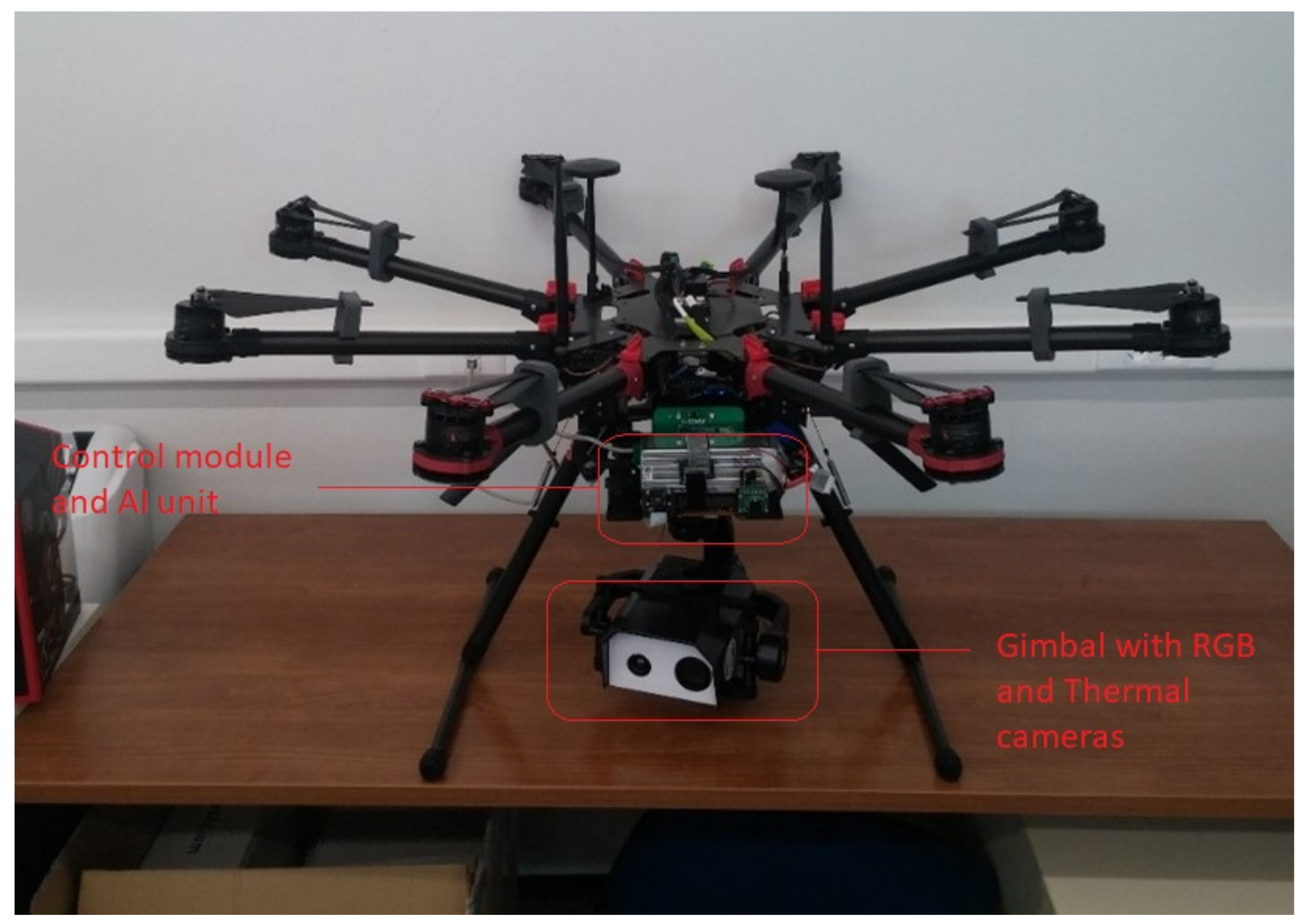
Figure 1.
The specially designed octocopter UAV showing the processing module container at its central unit, as well as the gimbal that carries the thermal and RGB cameras suspended underneath.
Figure 1.
The specially designed octocopter UAV showing the processing module container at its central unit, as well as the gimbal that carries the thermal and RGB cameras suspended underneath.
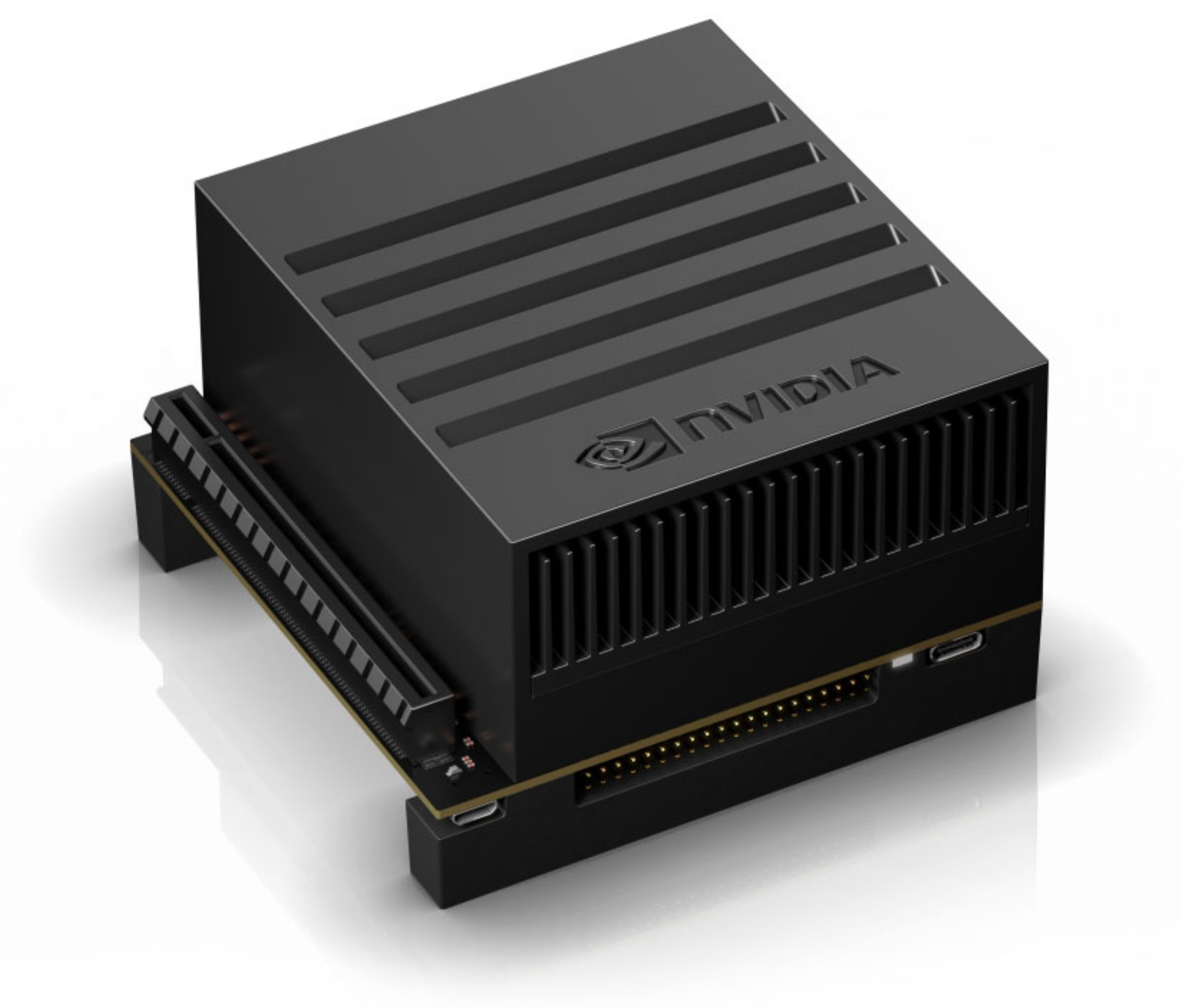
Figure 2.
The Jetson AGX Xavier module.
Figure 2.
The Jetson AGX Xavier module.
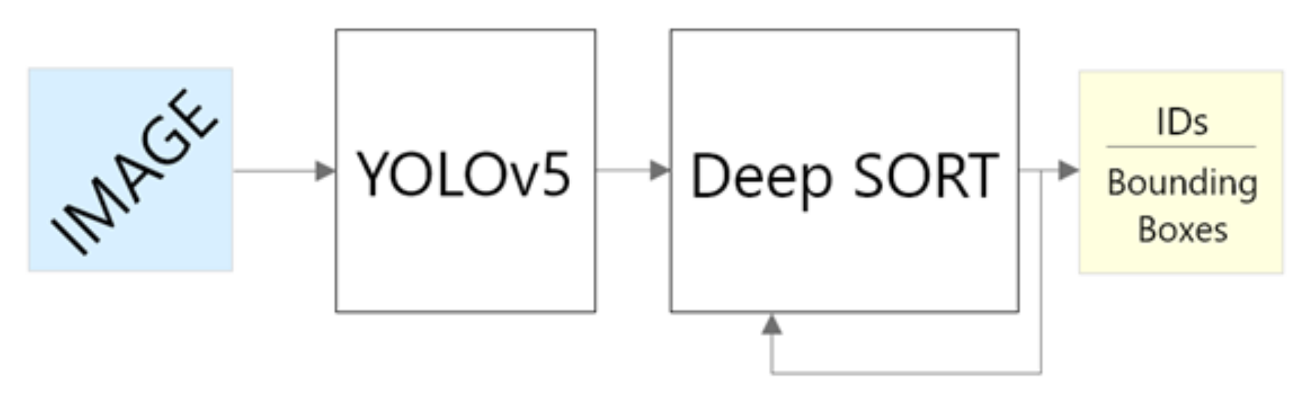
Figure 3.
The general architecture showing the distinct components of the system. An image is fed to YOLOv5, and detections are passed to the DeepSORT tracking algorithm. IDs and bounding boxes are retained as the object is tracked.
Figure 3.
The general architecture showing the distinct components of the system. An image is fed to YOLOv5, and detections are passed to the DeepSORT tracking algorithm. IDs and bounding boxes are retained as the object is tracked.
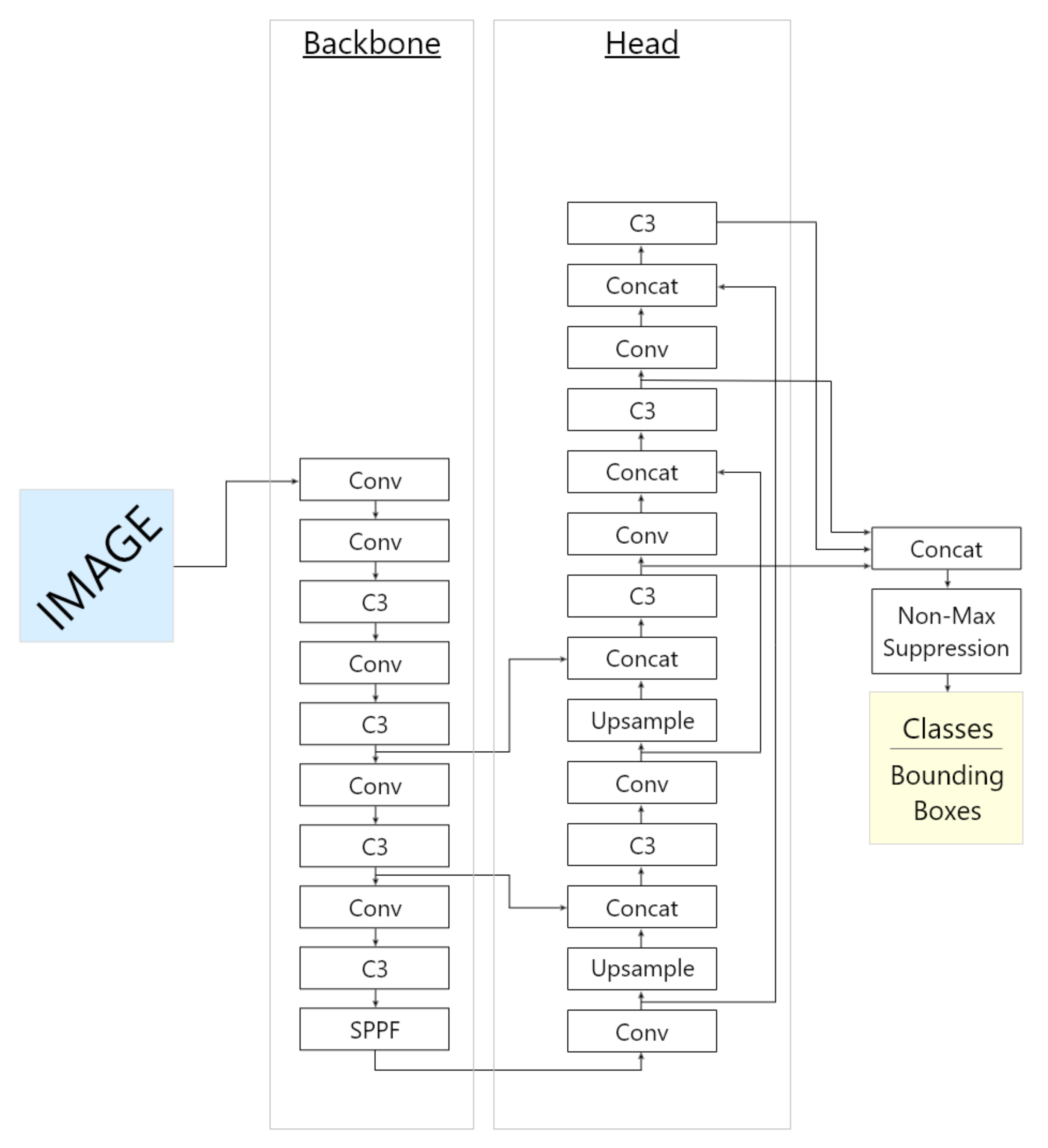
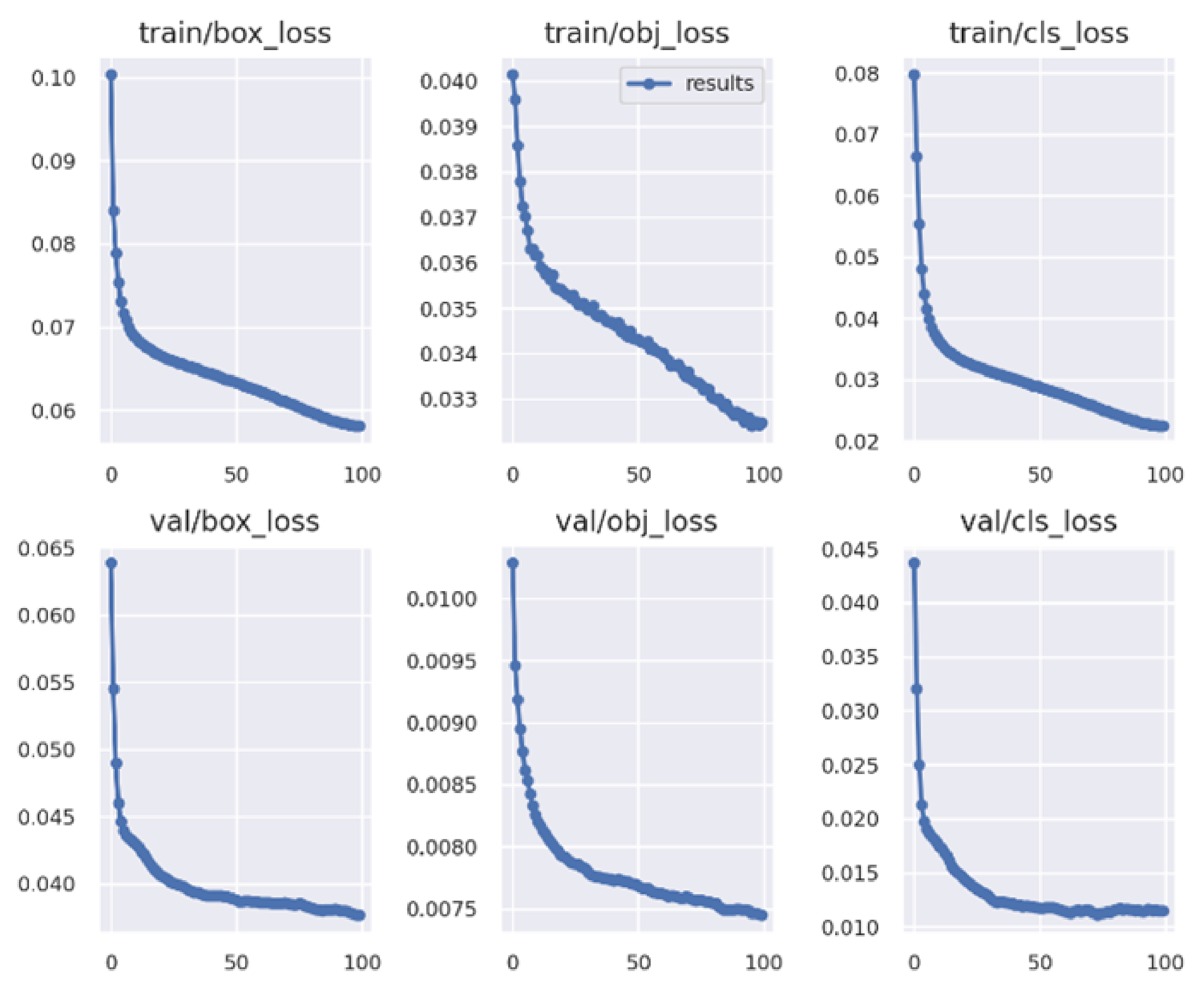
Figure 4.
YOLOv5 architecture.
Figure 4.
YOLOv5 architecture.
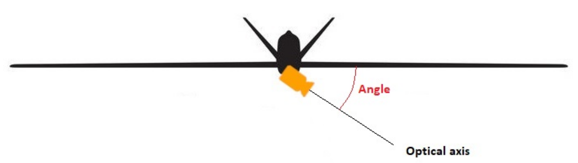
Figure 5.
UAV camera position on the UAV showing the angle of the optical axis (direction where the camera is targeted) relative to the plane of the UAV. An angle of 90
between the two means that the camera is pointing directly downwards. (Source: [
20]).
Figure 5.
UAV camera position on the UAV showing the angle of the optical axis (direction where the camera is targeted) relative to the plane of the UAV. An angle of 90
between the two means that the camera is pointing directly downwards. (Source: [
20]).
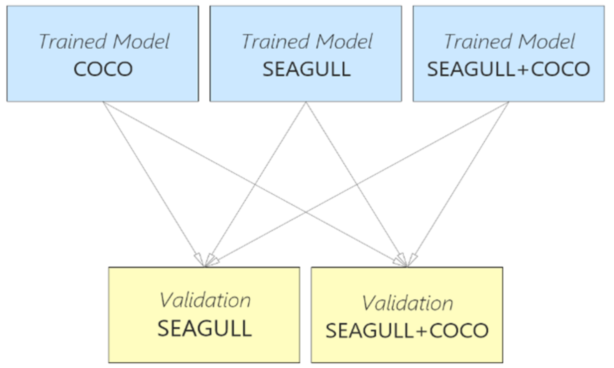
Figure 6.
Tested combinations between algorithms and datasets.
Figure 6.
Tested combinations between algorithms and datasets.
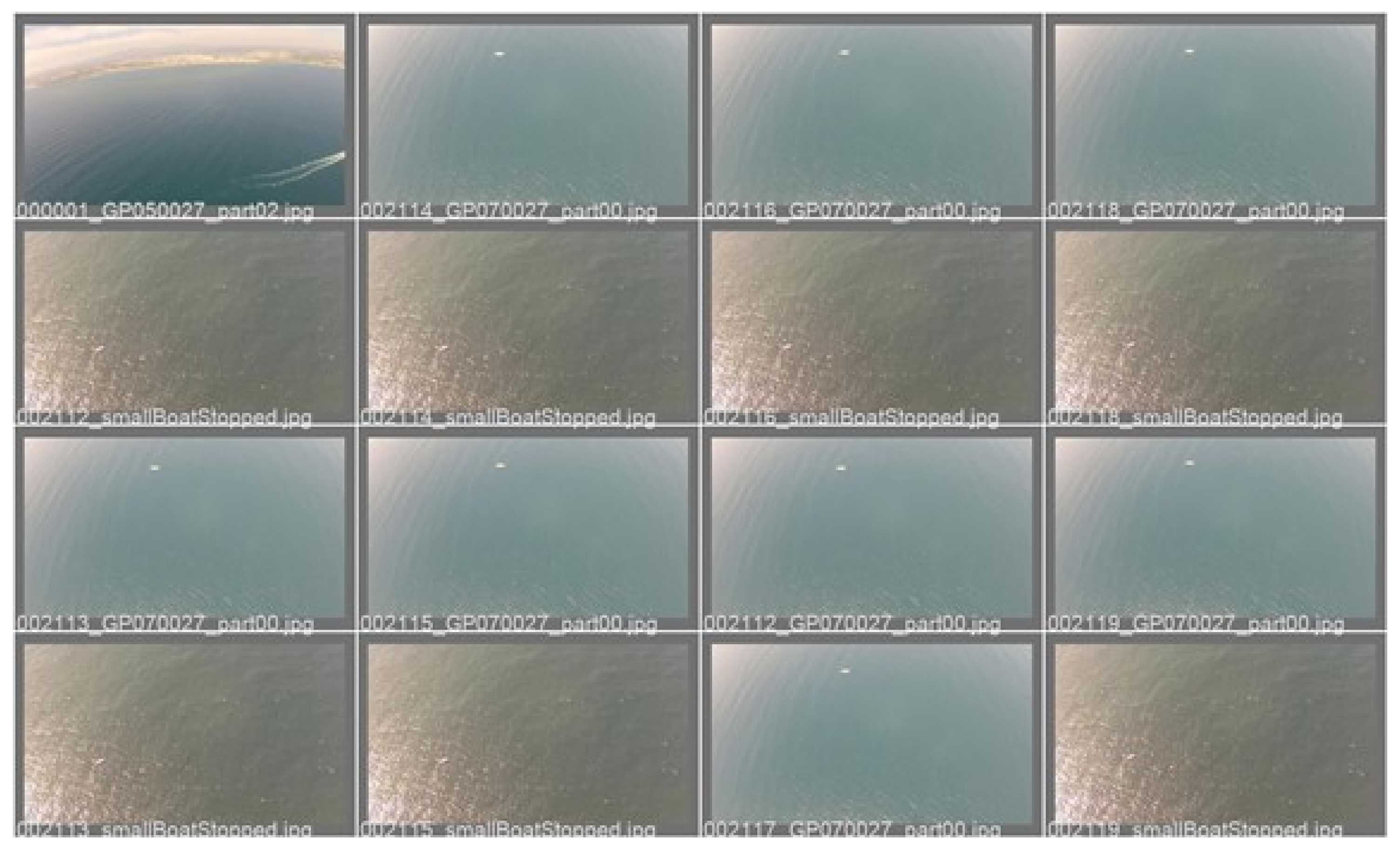
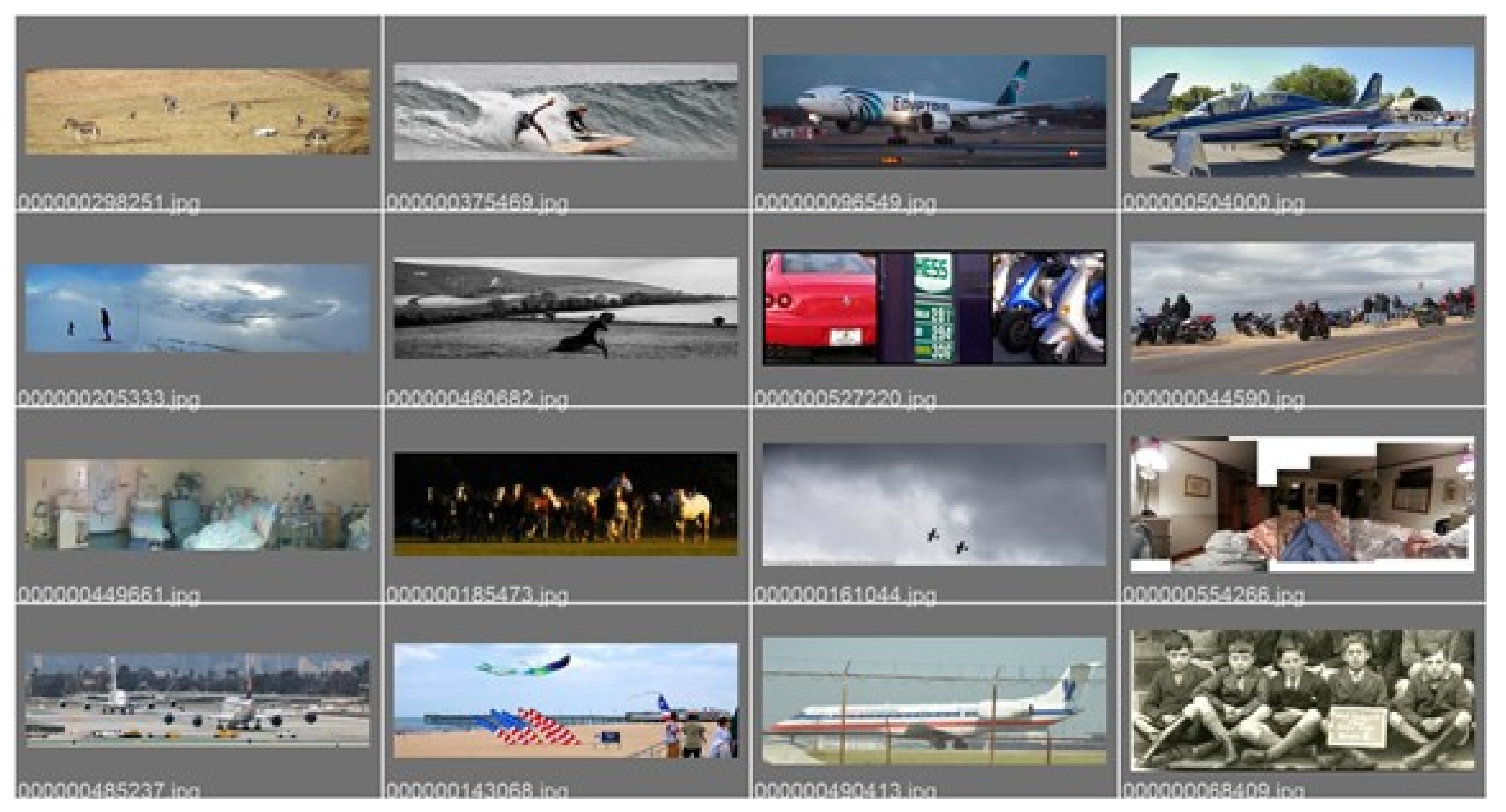
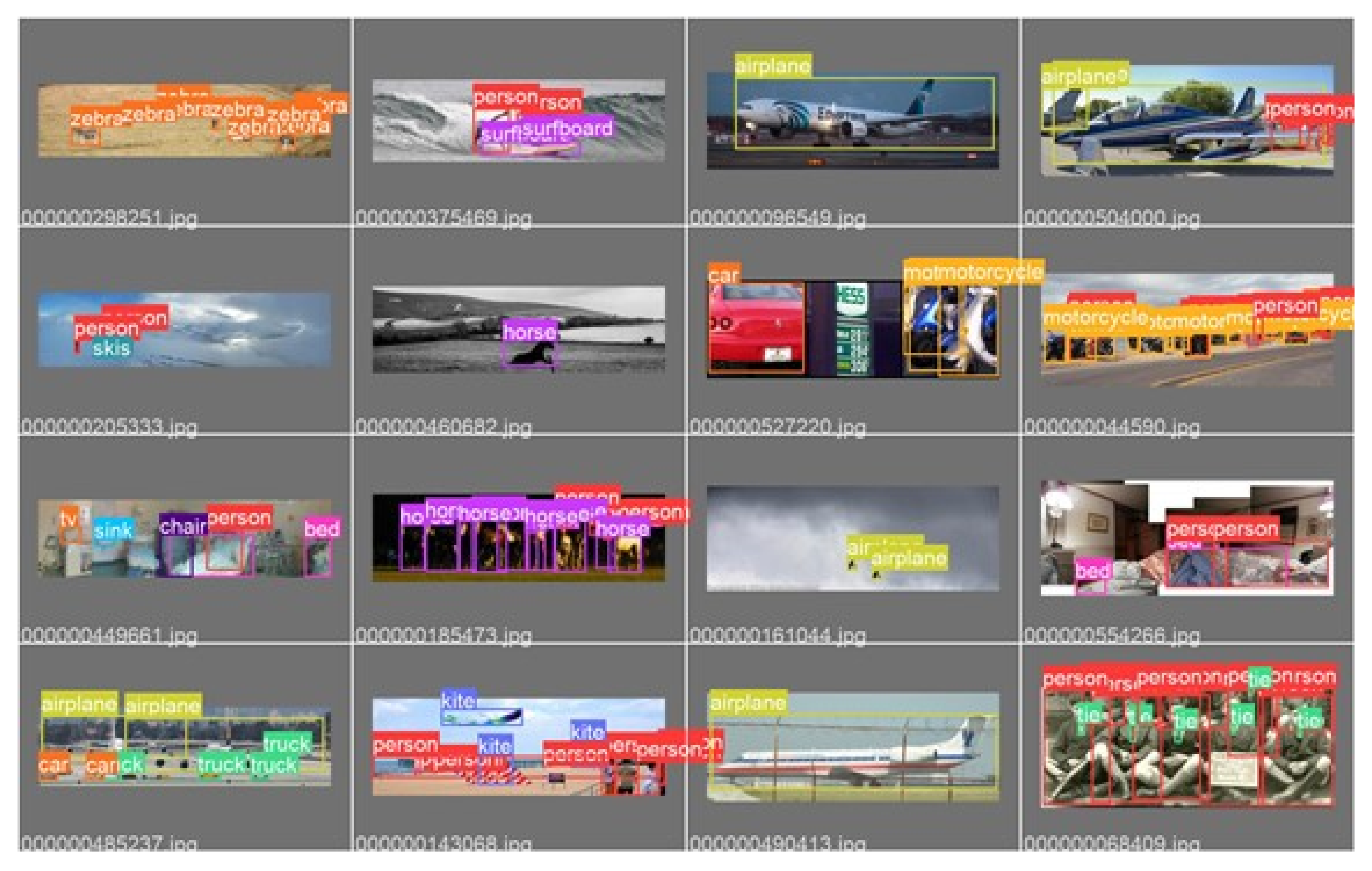
Figure 7.
Examples of annotated images in the test set from SEAGULL—ground truth bounding boxes visible.
Figure 7.
Examples of annotated images in the test set from SEAGULL—ground truth bounding boxes visible.
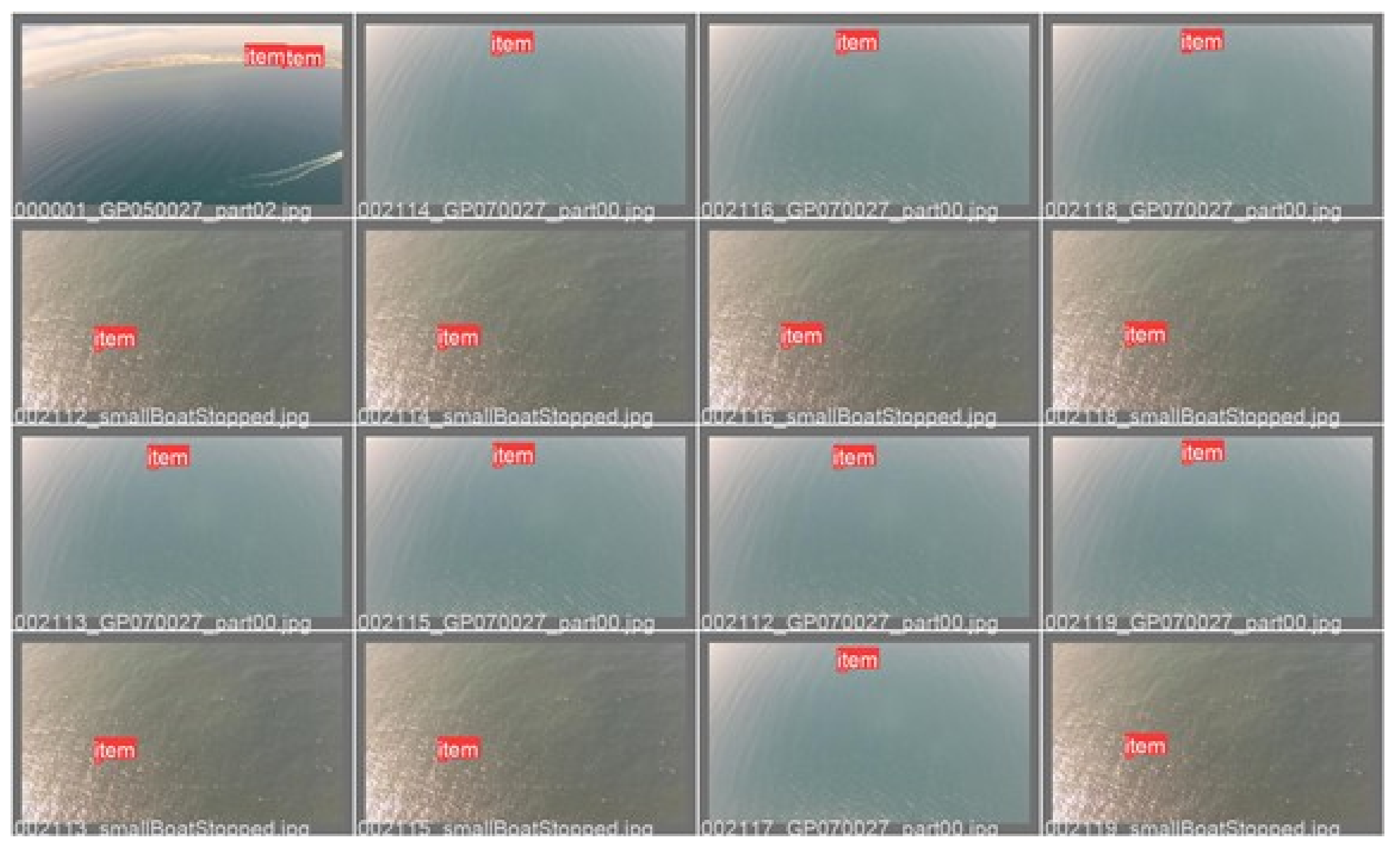
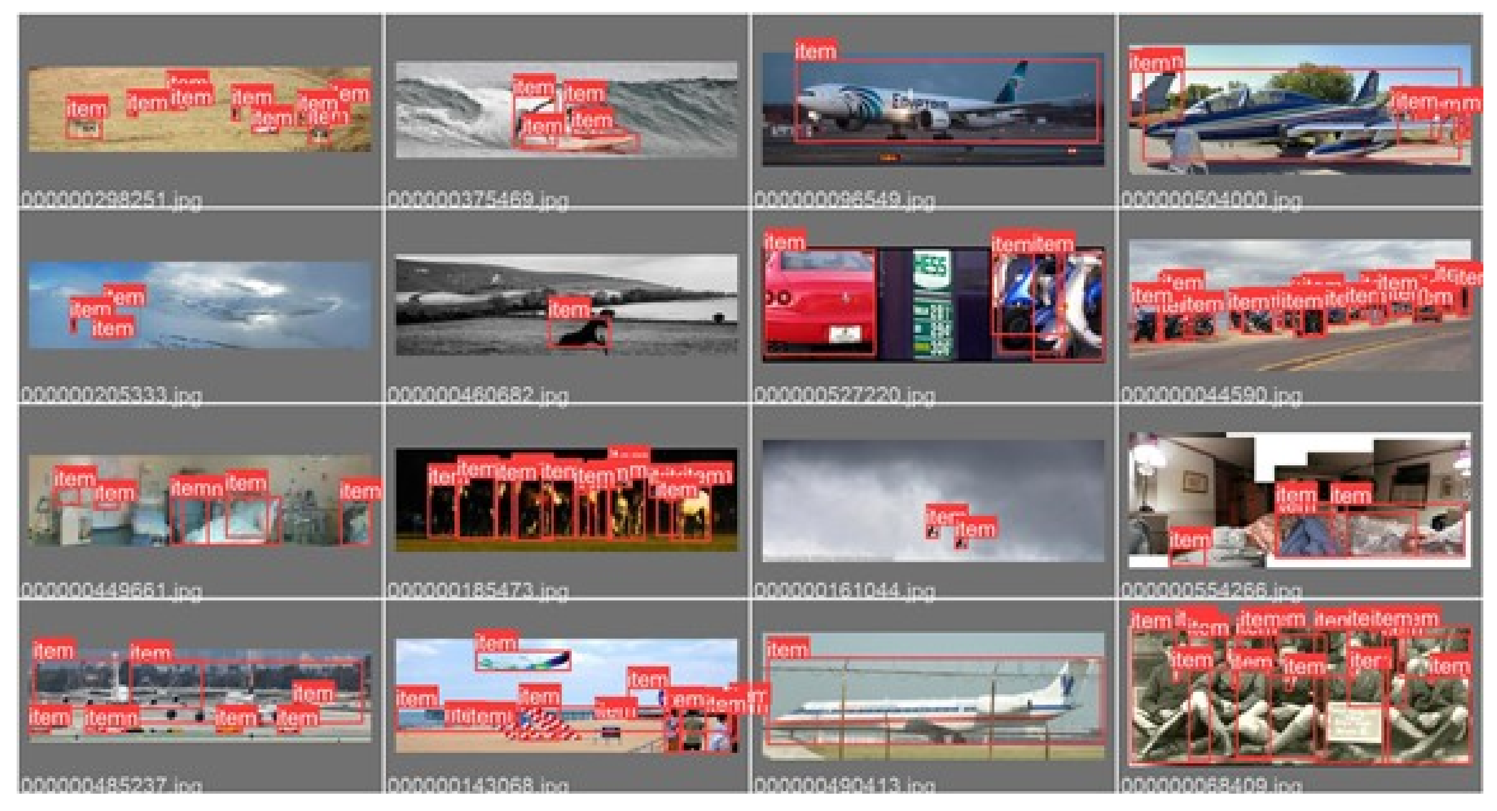
Figure 8.
Examples of annotated images in the test set from SEAGULL—the pretrained algorithm failed to predict bounding boxes in all test images.
Figure 8.
Examples of annotated images in the test set from SEAGULL—the pretrained algorithm failed to predict bounding boxes in all test images.
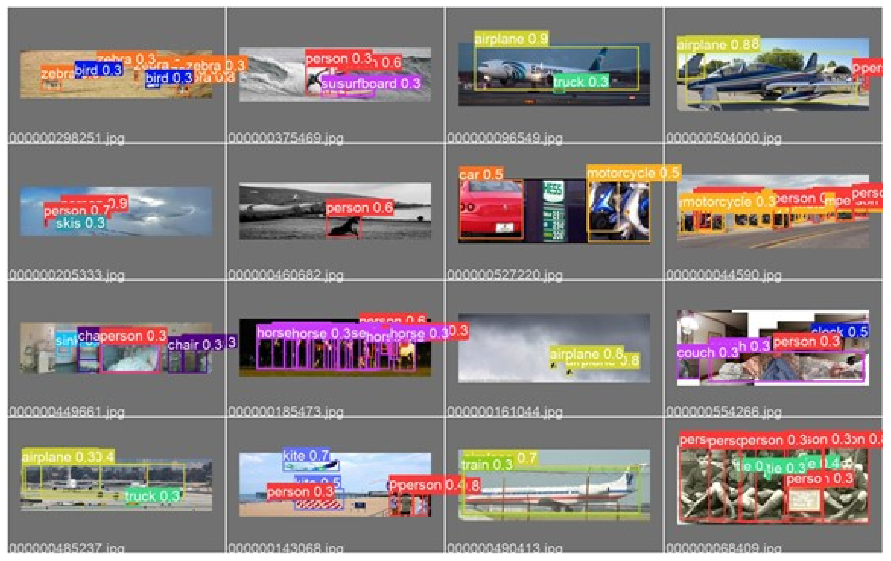
Figure 9.
Examples of annotated images in the test set from the COCO and SEAGULL combination—ground truth bounding boxes visible.
Figure 9.
Examples of annotated images in the test set from the COCO and SEAGULL combination—ground truth bounding boxes visible.
Figure 10.
Examples of annotated images in the test set from the COCO and SEAGULL combination—the pretrained algorithm failed to predict bounding boxes in all test images.
Figure 10.
Examples of annotated images in the test set from the COCO and SEAGULL combination—the pretrained algorithm failed to predict bounding boxes in all test images.
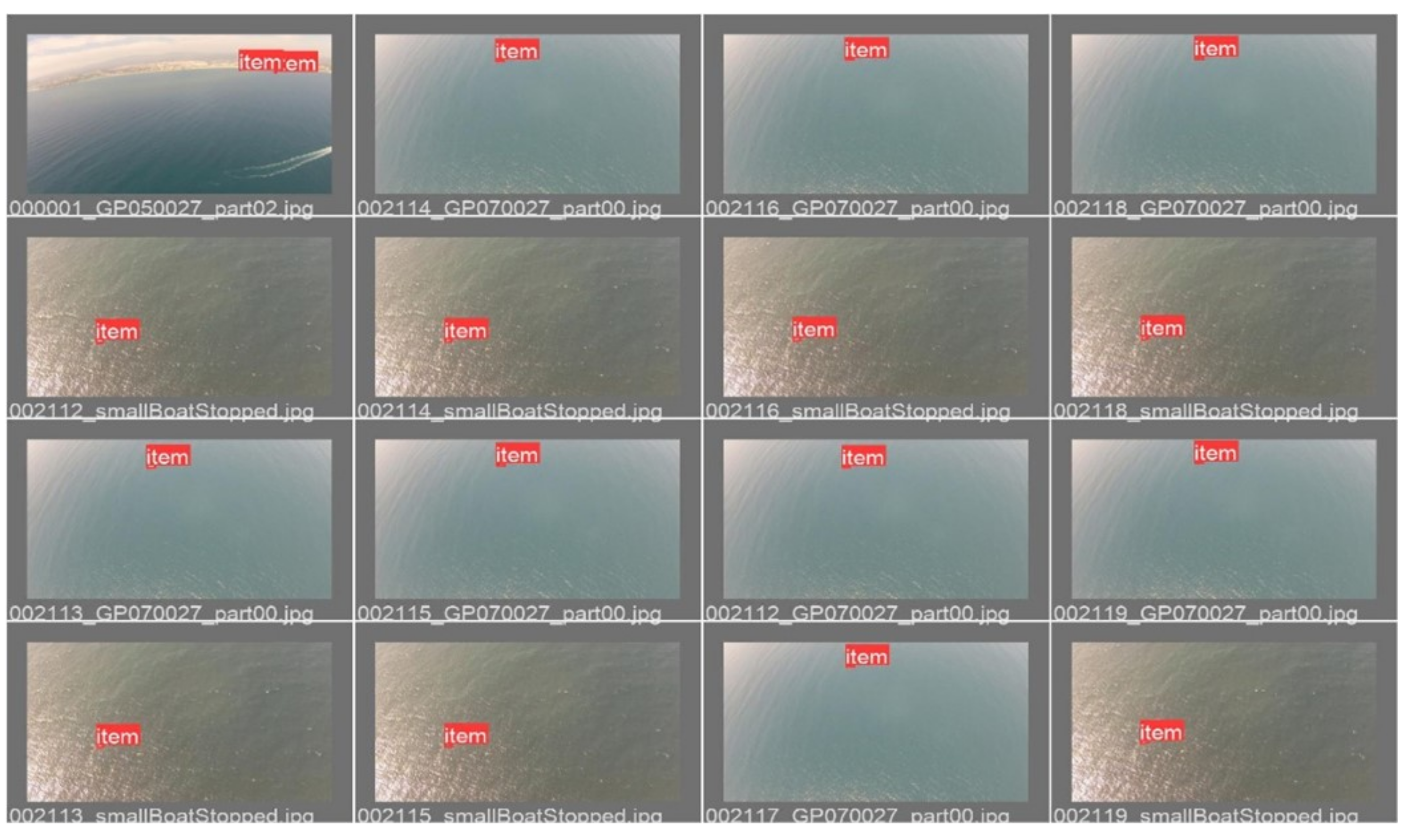
Figure 11.
Examples of annotated images from the SEAGULL test set—ground truth bounding boxes visible.
Figure 11.
Examples of annotated images from the SEAGULL test set—ground truth bounding boxes visible.
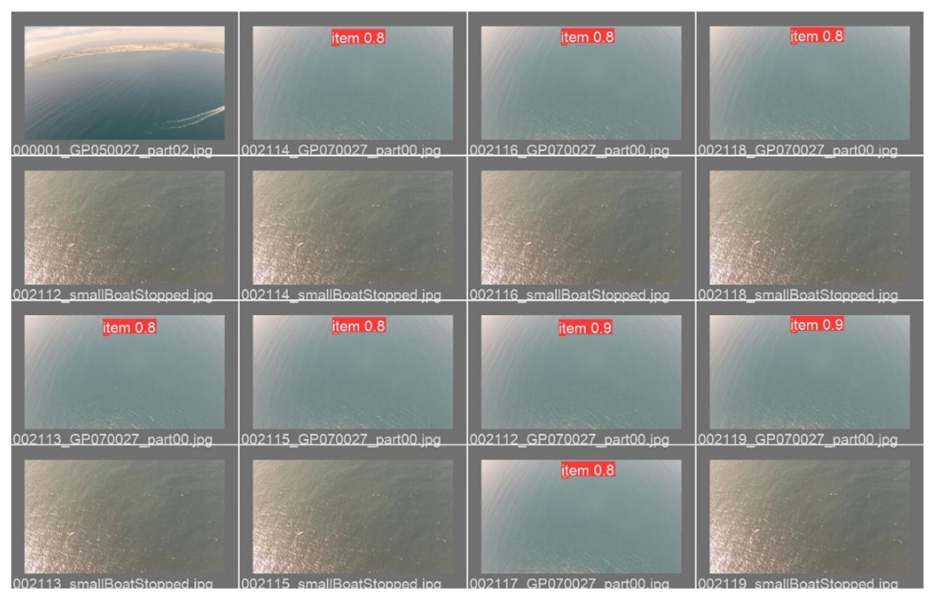
Figure 12.
Examples of annotated images from the SEAGULL test set—predicted bounding boxes with the confidence visible as drawn by the algorithm trained on SEAGULL alone.
Figure 12.
Examples of annotated images from the SEAGULL test set—predicted bounding boxes with the confidence visible as drawn by the algorithm trained on SEAGULL alone.
Figure 13.
Training on the SEAGULL—progress of metrics during the 100 epochs.
Figure 13.
Training on the SEAGULL—progress of metrics during the 100 epochs.
Figure 14.
Training on the SEAGULL—progress of metrics during the 100 epochs.
Figure 14.
Training on the SEAGULL—progress of metrics during the 100 epochs.
Figure 15.
Examples of annotated images from the COCO test set—ground truth bounding boxes and classes visible.
Figure 15.
Examples of annotated images from the COCO test set—ground truth bounding boxes and classes visible.
Figure 16.
Examples of annotated images in the test set from the COCO and SEAGULL combination—bounding boxes and classes with confidence shown as predicted by the algorithm trained on the combined dataset.
Figure 16.
Examples of annotated images in the test set from the COCO and SEAGULL combination—bounding boxes and classes with confidence shown as predicted by the algorithm trained on the combined dataset.
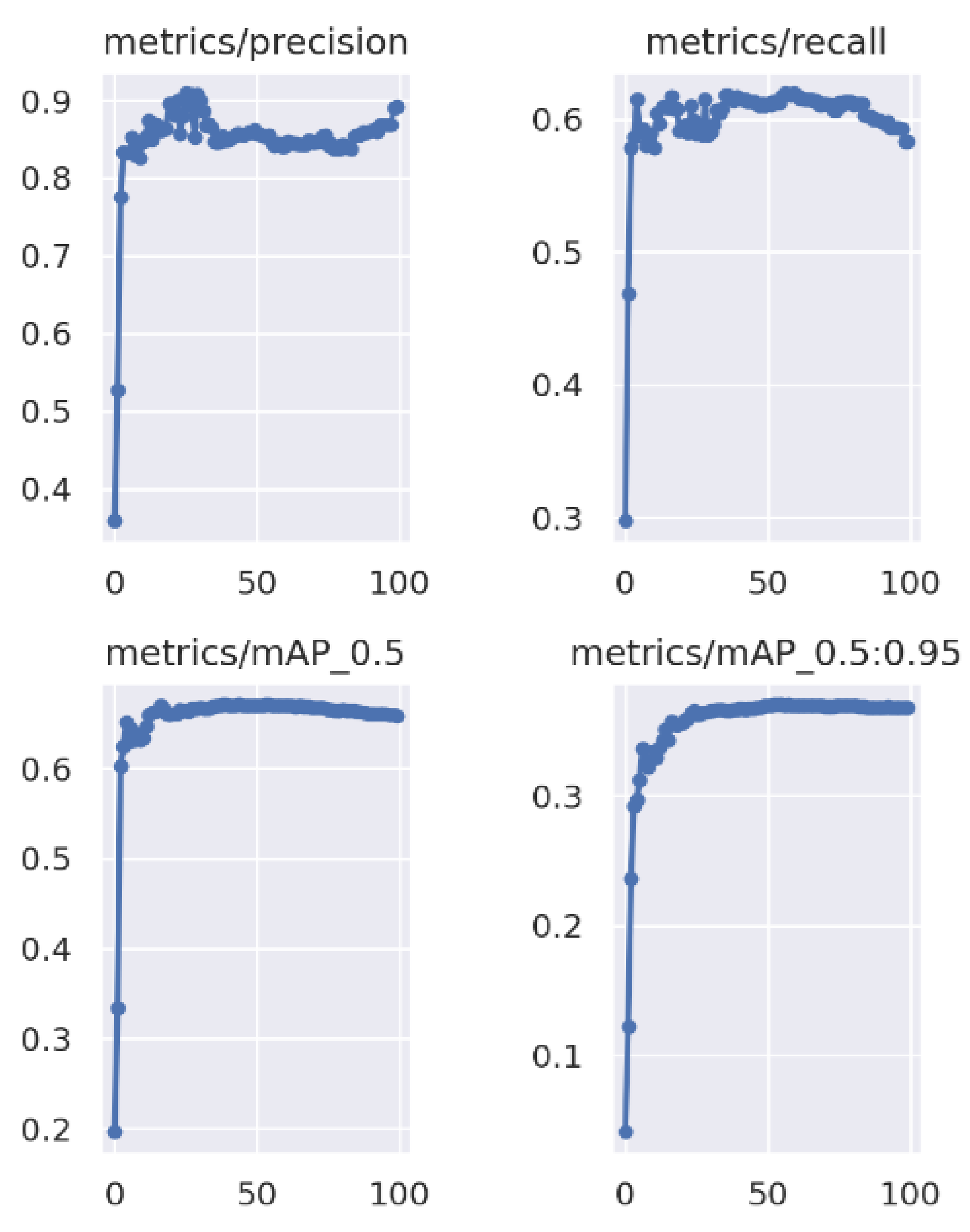
Figure 17.
Training on the SEAGULL and COCO combination—progress of metrics during the 100 epochs.
Figure 17.
Training on the SEAGULL and COCO combination—progress of metrics during the 100 epochs.
Figure 18.
Training on the SEAGULL and COCO combination—progress of metrics during the 100 epochs.
Figure 18.
Training on the SEAGULL and COCO combination—progress of metrics during the 100 epochs.
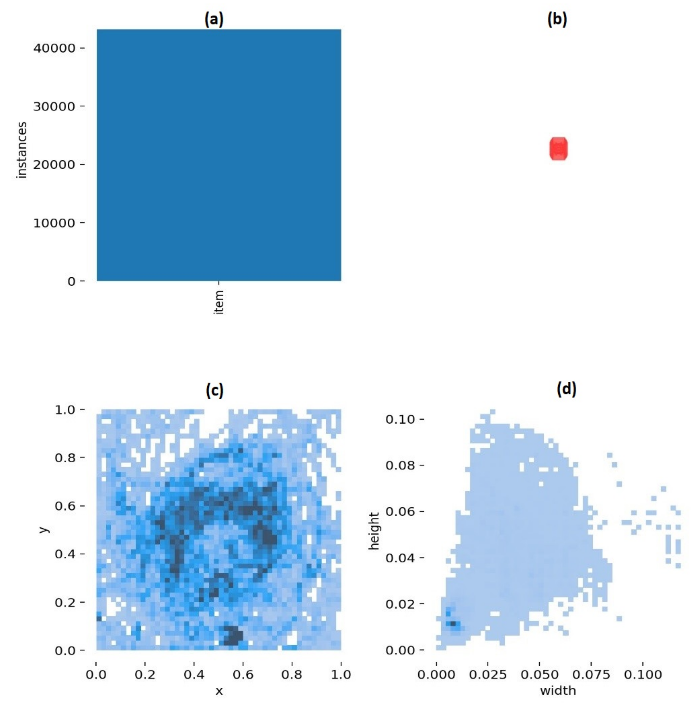
Figure 19.
Model trained on SEAGULL—(a) number of training items in the dataset, (b) anchor boxes used for the final bounding boxes, i.e., the detections, (c) frequency of the central positions of the objects of the dataset, (d) size of the bounding boxes as a percentage of the images’ width and height for the SEAGULL- and SEAGULL+COCO-trained models, respectively.
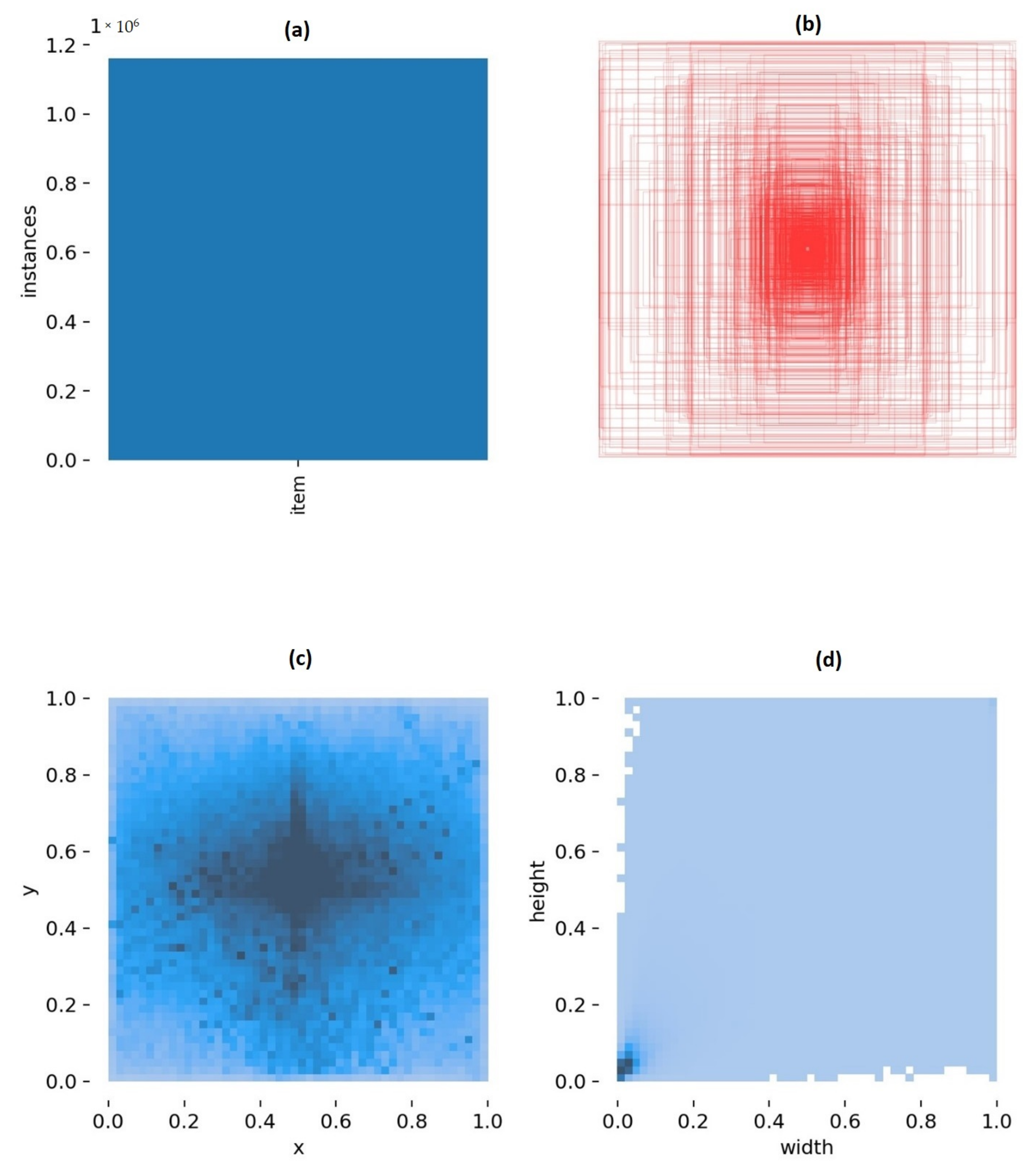
Figure 20.
Model trained on SEAGULL and COCO—(a) number of training items in the dataset, (b) anchor boxes used for the final bounding boxes, i.e., the detections, (c) frequency of the central positions of the objects of the dataset, (d) size of the bounding boxes as a percentage of the images’ width and height for the SEAGULL- and SEAGULL+COCO-trained models, respectively.
Table 1.
Technical specifications of the Jetson AGX Xavier module.
Table 1.
Technical specifications of the Jetson AGX Xavier module.
| GPU | 512-core Volta GPU with Tensor Cores |
| CPU | 8-core ARM v8.2 64 bit CPU, 8MB L2 + 4MB L3 |
| Memory | 32 GB 256 bit LPDDR4x | 137 GB/s |
| Storage | 32 GB eMMC 5.1 |
| DL accelerator | (2×) NVDLA Engines |
| Vision accelerator | 7-way VLIW Vision Processor |
| Encoder/decoder | (2×) 4Kp60 | HEVC/(2×) 4Kp60 | 12 bit Support |
| Size | 105 mm × 105 mm × 65 mm |
| Deployment | Module (Jetson AGX Xavier) |
Table 2.
Basic training hyperparameters.
Table 2.
Basic training hyperparameters.
| Epochs | 100 |
| Batch size | 32 |
| Image size | 448 |
| Optimizer | SGD |
| Learning rate | 0.01 |
| Momentum | 0.937 |
Table 3.
Validation on SEAGULL—values of metrics.
Table 3.
Validation on SEAGULL—values of metrics.
| mAP_0.5 | 0.00002 |
| mAP_0.5:0.95e | 0.000005 |
| Box loss | 0.16 |
| obj loss | 0.013 |
Table 4.
Validation on SEAGULL and COCO combination—values of metrics.
Table 4.
Validation on SEAGULL and COCO combination—values of metrics.
| mAP_0.5 | 0.0015 |
| mAP_0.5:0.95e | 0.0003 |
| Box loss | 0.20 |
| obj loss | 0.018 |
Table 5.
Validation on SEAGULL—optimal values of metrics.
Table 5.
Validation on SEAGULL—optimal values of metrics.
| mAP_0.5 | 0.67 |
| mAP_0.5:0.95e | 0.357 |
| Box loss | 0.057 |
| obj loss | 0.0045 |
Table 6.
Validation on SEAGULL and COCO combination—values of metrics.
Table 6.
Validation on SEAGULL and COCO combination—values of metrics.
| mAP_0.5 | 0.31471 |
| mAP_0.5:0.95e | 0.12733 |
| Box loss | 0.055589 |
| obj loss | 0.0093003 |
Table 7.
Validation on SEAGULL and COCO combination—values of metrics.
Table 7.
Validation on SEAGULL and COCO combination—values of metrics.
| mAP_0.5 | 0.50 |
| mAP_0.5:0.95e | 0.32 |
| Box loss | 0.037 |
| obj loss | 0.007 |
Table 8.
Validation on SEAGULL—values of metrics.
Table 8.
Validation on SEAGULL—values of metrics.
| mAP_0.5 | 0.66 |
| mAP_0.5:0.95e | 0.337 |
| Box loss | 0.031 |
| obj loss | 0.0034 |
Table 9.
Comparison of metrics between the small and medium versions of YOLOv5.
Table 9.
Comparison of metrics between the small and medium versions of YOLOv5.
| Metrics | Small YOLOv5 | Medium YOLOv5 |
|---|
| mAP_0.5 | 0.50 | 0.57 |
| mAP_0.5:0.95e | 0.32 | 0.38 |
| Box loss | 0.037 | 0.034 |
| obj loss | 0.007 | 0.007 |


 ,
, 


