Numerical Study of the Influence of the Geometrical Irregularities on Bodies of Revolution at High Angles of Attack

Abstract

The flow at high angles of attack over axisymmetric configurations is not symmetric. The mechanism that triggers the asymmetry may be a combination of a global or hydrodynamic instability (temporal instability) combined with a convective instability (spatial instability) due to microscopic irregularities of the configuration. Poor repeatability of experiments and large differences in the global forces have been obtained with very small changes of the nose tip. In order to study theoretically this phenomenon, numerical simulations have been conducted for an ogive-cylinder configuration at subsonic flow and high angle of attack. For the numerical prediction of the flow about a missile type configuration, an assessment of the effect of structured and unstructured meshes is very important. How the body surface is modelled is very relevant; especially the tip zone of the body. Either configuration resembles a smooth or a rough model. The effect of the turbulence models is also decisive. The analysis has led to the conclusion that only Reynolds stress turbulence models (RSM) combined with Scale Adaptive Simulation (SAS), are the appropriate theoretical tools for the characterization of this flow. The geometrical similarity is very important. There is a roll or orientation angle effect for the unstructured grid, while the structured grid presents a bi-stable solution, one mirror of each other.

1. Introduction

The numerical simulation of the flow field about an axisymmetric body flying at high angle of attack and subsonic flow conditions is a challenging problem, since it entails large areas of boundary layer separation and a complex vortex sheet structure. At low angles of attack the flow is attached to the body, developing a normal force which increases linearly with the angle of attack. At intermediate angles the increasing adverse pressure gradients on the body surface force the leeside boundary layer to separate. The normal force then evolves in a nonlinear manner, but there is still no side force. At larger angles the axial flow is still sufficiently effective to produce an asymmetric flow pattern leading to the appearance of a side force. At very large angles the boundary layer is shed in an unsteady fashion, similar to the wake behind a 2D cylinder normal to the flow, the average side force decaying to zero.

There are two dimensionless parameters of the flow domain that affect this basic flow structure: Mach number and Reynolds number. Regarding the Mach number, the asymmetry of the flow disappears as the Mach number increases. The appearance of shocks at the leeward side makes the flow symmetric [1]. Concerning Reynolds number effects, it has been demonstrated in several experimental tests that maximum side forces occur both at laminar or turbulent flow conditions. This behavior reinforces the idea that a global instability of inviscid nature is the origin of the asymmetry [1]. Experiments conducted by Lamont [2] showed this effect: the side forces are reduced in the critical Reynolds number region.

Moreover, some geometric characteristics are relevant for the flow structure: nose angle, bluntness, fineness ratio and roughness. The nose angle appears to be a relevant factor. Keener and Chapman [3] introduced the idea of a hydrodynamic (inviscid) mechanism as the origin of the asymmetry. The asymmetric wake is the result of an inviscid instability that occurs when two vortices are “crowded together” near the tip of the body. One vortex moves away from the body and the other moves underneath the first. Champigny [1] shows that above a certain angle of attack, very small perturbations (inhomogeneities in the mainstream, surface irregularities, geometrical defects, etc.) are sufficient to cause the vortex system to go from an unstable symmetric state to a stable asymmetric structure. There are two specular but otherwise similar flow field structures.

Roughness or small eccentricities or other geometrical body imperfections are also relevant factors in the appearance of asymmetric flow patterns. At a certain angle of attack, experiments have shown that the side forces depend on the orientation angle [1,4,5,6,7]. Two different series of experiments, one described by P. Champigny on an ogive cylinder configuration (Refs. [1,6]) and another conducted by Mahadevan et al. on a cone configuration (Ref. [7]), reported different orientation angle effects on the side force depending on the roughness of the model. The results for the ogive cylinder showed a bi-stable behavior for smooth surfaces while for a rough surface the side force depended on the orientation angle, leading to large variations of the side force magnitude. Similarly, the results of the rough surface model of a cone [7] showed a sinusoidal variation of the side force with the orientation angle, while there is a bi-stable pattern of the side force at the range of moderate to high angles of attack for the smooth surface model.

Experiments conducted by Kruse, Keener and Chapman [5] showed that rotating the tip of an axisymmetric body has large effects on the side forces; the rotation of the afterbody (cylindrical part) holding the tip had also a large effect on these side forces. Then, minor surface irregularities may cause the activation of a convective instability, also in zones far from the tip. The result is a dependence of the side force on the orientation angle.

A convective instability is defined by three major features, according to Bridges [8]: (i) an asymmetrical infinitesimal disturbance develops a side force of finite magnitude (ii) a minute change in magnitude of the disturbance results in a finite change in the asymmetric component, sometimes to the extent of reversing the sign of the side force, and (iii) when the fixed disturbance is removed, the perturbed flow relaxes back to the original state. It is thought that roughness can have an important effect in activating this convective instability at large angles of attack, as experiments have shown (see [1,5,7]).

The purpose of this study is to assess the capability of Unsteady Reynolds Averaged Navier-Stokes (URANS) methods to predict the main features of the asymmetric flow at high angles of attack and subsonic flow conditions for axisymmetric bodies. To do that, the calculations have been done using an ogive-cylinder body of moderate fineness ratio for which abundant experimental data are available: global forces, local forces and also pressure coefficients at several axial sections [9,10].

In this numerical study, a study of the roughness of the configurations used for the calculations has been conducted. As two test models were used in the experiments -one smooth or polished model and another rough model—two different meshes—structured and unstructured grids- were used in order to study the influence of the surface imperfections on the side force. The procedure used for the unstructured grids led to surface irregularities such that resemble a rough model. The structured grid was built rotating a two-dimensional mesh about the longitudinal axis to create an axisymmetric mesh. Therefore, the surface irregularities of this structured surface grid were much smaller and resemble a smooth configuration.

2. Test Case: Ogive-Cylinder at Subsonic Flow

A configuration with abundant experimental data was used as test case. Thus, our numerical results are compared to the experimental data of an ogive-cylinder configuration tested by ONERA (Office National d’Etudes et de Recherches Aérospatiales) [1,9,10].

The test model consisted of a 120 mm diameter cylindrical body with a 3-calibre tangent ogive nose. The total length was 15 calibers (L/D = 15). This ogive-cylinder configuration was tested in the ONERA F1 pressurized wind tunnel at Le Fauge-Mauzac (France). The flow conditions for the reference case were Mach number Ma = 0.2, Reynolds number Re = 2∙10⁶ and angle of attack α = 45.43 degrees. Results at other angles of attack were also available. The diameter of the configuration under study was D = 1 m. The temperature of the air was T = 288 °K and the pressure and density were adjusted to obtain a Reynolds number similar to that of the experiments. For the theoretical study, the reference case flow conditions were finally Ma = 0.20, Re = 2.2 × 10⁶ and α = 45.00 degrees. Also, a sweep in angle of attack was done, from low values and up to 45 degrees. A theoretical study using different codes with several turbulence models and different grids was done under a GARTEUR Research Group, led by Prananta [10]. This study has been very useful for the present work and helped to do the comparison with the experimental data and to obtain conclusions about the different turbulence models. In reference [9] abundant experimental data at different Mach and Reynolds numbers is given for a smooth and a rough model. The smooth model is the original test model, while the rough model is the result of painting and mechanizing pressure taps. There is no information in this reference [9] about the roughness or orientation angle effects, but in reference [1] results of the side force versus orientation angle for the smooth and rough model are shown. The side force of the smooth model has a bi-stable pattern while the rough model shows a sinusoidal and continuous variation of the side force with the orientation angle. The average roughness of the smooth model is Ra/D = 5 × 10⁻⁶ and the average roughness of the rough model is Ra/D = 40 × 10⁻⁶. This is very important for the comparison with the theoretical solutions given by two different meshes, structured and unstructured grids, which resemble a smooth and a rough model respectively, as it can be shown below.

3. Grids: Numerical Roughness

Two grids were built for the calculations. One grid is a structured axisymmetric grid and the other is an unstructured hybrid grid, composed by prismatic and tetrahedral elements.

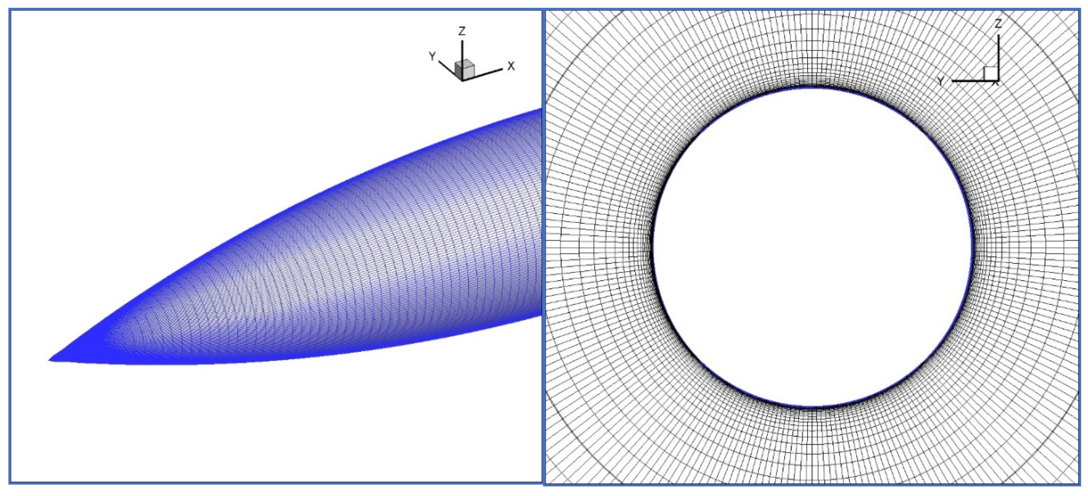
Regarding the structured grid, a two-dimensional structured grid was firstly built up. Then, this planar two-dimensional grid was rotated every n degrees. The total number of cells in azimuth direction is $\raisebox{1ex}{$360$}\!\left/ \!\raisebox{-1ex}{$N$}\right.$. This number N was usually chosen as 240 or 360. The grid with 240 cells in azimuth direction was the grid utilized as reference grid for the calculations. The structured grid finally used has 450 cells in the longitudinal direction (x-axis direction), 140 in normal direction and 240 in azimuth direction. This grid is a fine mesh of 15,120,000 cells and 45,114,720 faces. A detail of this grid is shown in Figure 1. There is a stretching law in normal direction. The height of the first cell to the surface was chosen as 10⁻⁵ m. With this value, the y⁺ was of order 1. This is important for capturing the boundary layer with accuracy. The number of cells within the boundary layer was 32–48 depending on the axial position.

The unstructured grid was built up with a very different methodology, using a method to generate a surface mesh of a part of the ogive-cylinder covered by an angle $\mathsf{\Theta }=\frac{360}{m}$-being m an integer. This integer m can have any value. Values ranging from m = 3 to m = 8 have been used for the calculations shown in the present paper. A maximum cell size is chosen, together with other parameters. This method implies that in the sections x/D very close to the tip the grid is formed by a triangle if m = 3 and by an octagon if m = 8. When advancing in longitudinal direction a cross section will be formed by polygons of many elements which are closer to the ideal circular shape of the body in this sections. With the structured mesh, every section was formed by 240 or 360 elements, independent of the radius of the ideal circular section. For this unstructured mesh, this polygons have different number of elements and its distribution is not regular. The result is a surface mesh not axisymmetric, with cross sections different in number and distribution of the elements.

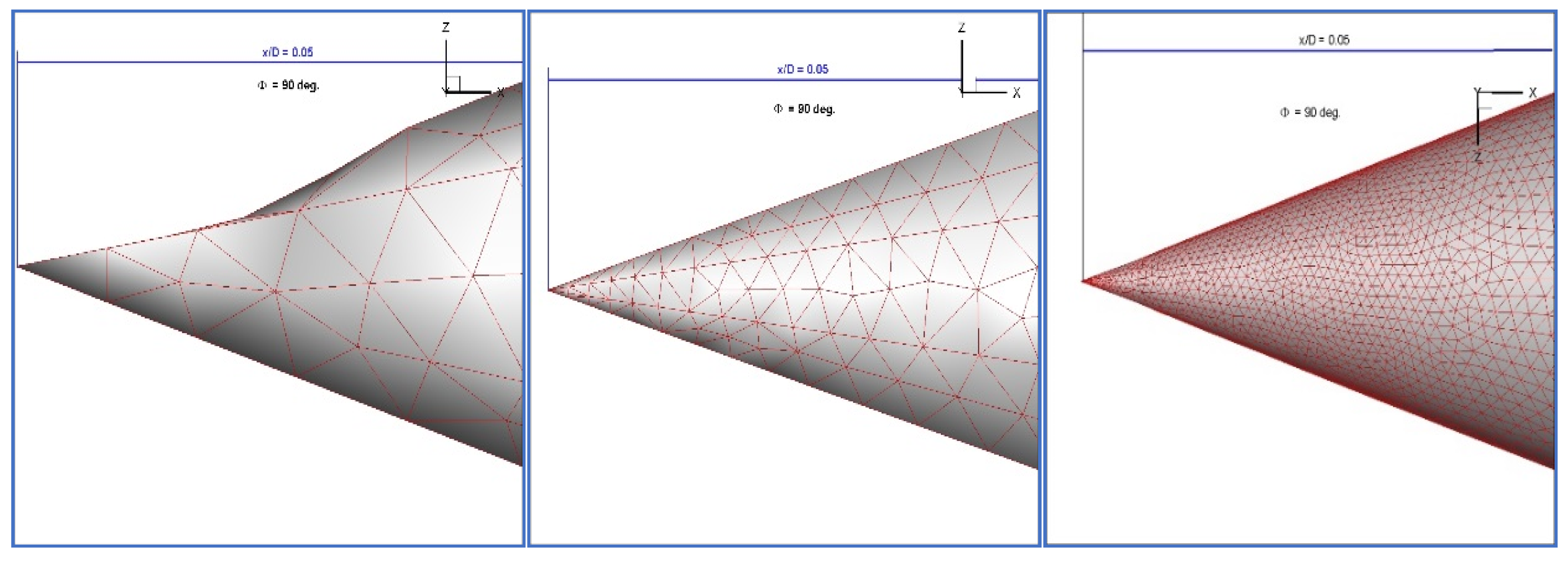
To give an insight of the implications of this type of meshing, a detail of the tip region is shown in Figure 2 for values of m = 3 and m = 8. The tip of the coarse mesh built up with m = 3 is very irregular. The tip of a grid generated with m = 8 is more regular but not axisymmetric. Finally, the finer grid of the right (m = 8) looks more symmetric; but, a detailed insight shows differences at each orientation angle. Therefore, neither of these grids are symmetric in the same fashion than the previously described structured grid.

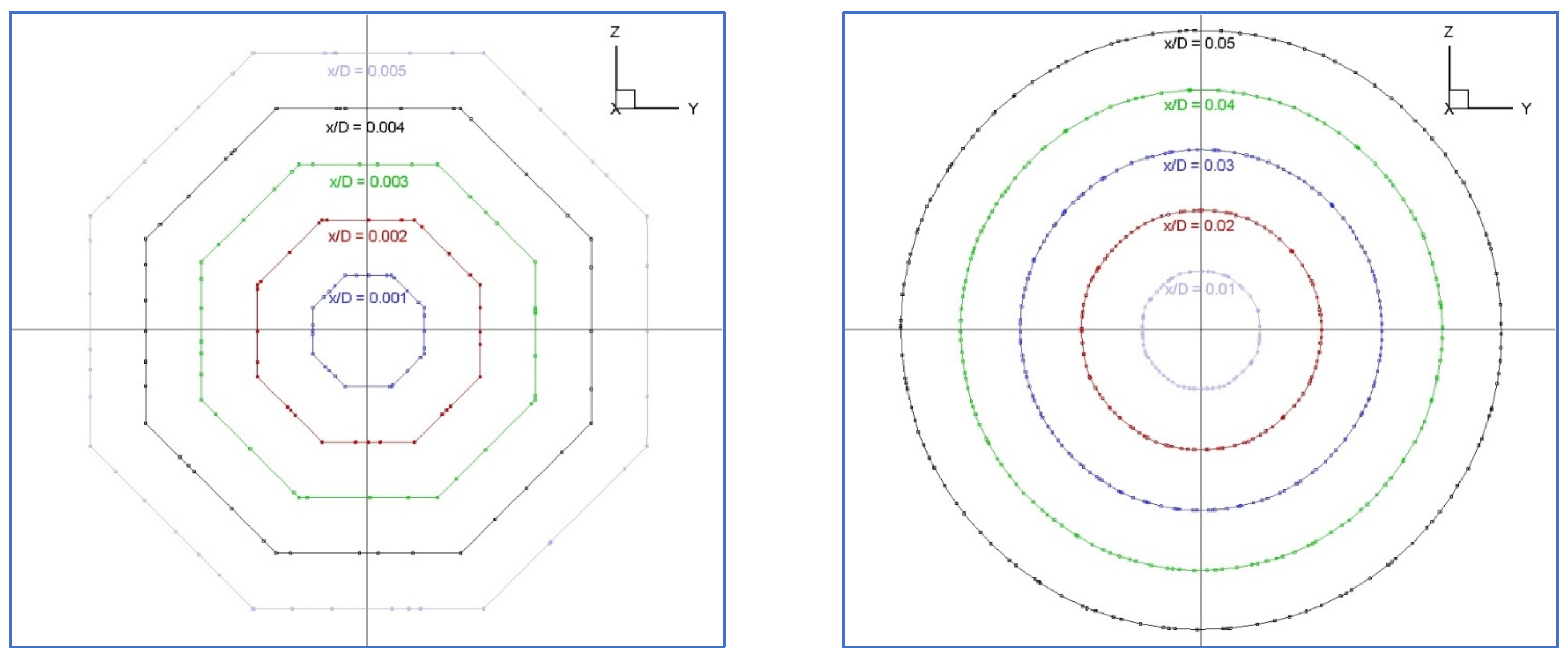
Regarding this mesh, it is interesting to show the surface grid in sections close to the tip. In the sections from x/D = 0.001 to x/D = 0.005 it can be seen Figure 3 (left) in that these sections are formed by octagons with the elements distributed differently and with different number of elements also. It can be seen in Figure 3 (right) that the cross sections evolve more uniformly and towards the ideal circular shape when advancing from x/D = 0.01 to x/D = 0.05.

These plots show clearly that the tip nose generated with this method is irregular and not symmetric. The roughness and microscopic irregularities, particularly in the tip region, are sources of a convective instability and may induce an important effect of the body orientation angle (i.e., the orientation angle of the grid with respect to the external flow field, being zero at the windward side) on the normal and lateral forces on the missile, as it has been widely demonstrated in many experiments [1,4,7,8].

In order to quantify the irregularities of the grids a ‘numerical roughness’ is defined in the following manner:

First of all, as the test model is a body of revolution, the average radius at each x/D section is defined as: $r_{avg}(x)=\frac{1}{N}{\displaystyle \sum _{i=1}^N{r}_i}(x)$. Then, the ‘numerical roughness’ at each section is calculated with the following expression: $\overline{r_n(x)}=\frac{1}{N}{\displaystyle \sum _{i=1}^N}\left|r_i(x)-r_{avg}(x)\right|$. This is an expression similar to that employed in [7]. The measurements at the different x/D sections show results of ‘numerical roughness’ between 40–60 × 10⁻⁶ m, i.e., r_n/D = 40–60 × 10⁻⁶. It should be noted that Mahadevan [7] defined a rough model with values of Ra/D > 60 × 10⁻⁶.

It can be concluded after the first analysis of the unstructured grid that the surface mesh generated with the procedure above mentioned, seems to resemble a model with a rough surface. As the volume mesh is also conditioned for the non-symmetric surface mesh, there will be also a non-symmetric volume mesh. The existence of a prismatic layer and tetrahedral elements in regions with strong pressure gradients and vortices of large strengths, may increase these irregularities effects coming from the surface. Therefore, orientation angle effects on the lateral forces can be predicted if the mesh resembles a rough model, while the structured grid can resemble a polished body, due to the axisymmetric nature of this mesh. A numerical study was conducted in order to check these possible effects.

4. CFD Computations: Accuracy and Validation

For the theoretical calculations, the well-known ANSYS FLUENT^© code was used [11]. This is a finite volume method which employs several algorithms for the calculation of the convective fluxes and iterative methods for achieving a solution, either a stationary or transient solution. For transient solutions, a dual time stepping method is used. For turbulence modelling, it is possible to use URANS or LES models. LES models are out of scope. For high Reynolds calculations, the grid size and time steps needed for accurate solutions lead to computing times several orders of magnitude larger compared to URANS method.

A study of the influence of turbulence modelling was carried out. Algebraic models or one equations models were considered not accurate enough for this type of flow. At high angles of attack there is massively separated flow at the leeside, and a complex vortex shedding. The conclusions of the CFD studies carried out for the same configuration under the GARTEUR Group AG42 were very useful to prepare our study (see Ref. [10]). Therefore, only eddy viscosity models based on ω (k-ω SST model for example) and Reynolds stress models were taken into account for the study. It is very important to notice that in the ANSYS FLUENT^© code, these type of models have been enhanced with SAS method. Scale Adaptive Simulation (SAS) is a model developed by Menter and Egorov [12,13,14,15]. A summary of the features of SAS is given in [13]: “SAS is an advanced URANS model which can produce spectral content for unstable flows”. The method is based on the introduction of a second length scale into the turbulence model, either a k-ω SST turbulence model, or a ω-based Reynolds Stress turbulence model (ω-RSM) [11]. This length scale is the von Karman length scale $L_{vk}$. This length scale adjusts to the smallest scales and produces an eddy viscosity small enough to allow the formation of even smaller eddies until the grid limit is reached [13]. Thus, SAS has a LES-like behavior in unstable regions of the flow and it works in RANS mode in the stable zones. It is worth noting that Menter and Egorov mention that “the ability of SAS to adjust the eddy-viscosity to the resolved scales is unique and cannot be achieved with standard LES models” [14]. If the grid is coarse or large time steps are used SAS model will run in RANS mode. One drawback of SAS model is that it relies on an instability of the flow to generate resolved turbulence. In case such an instability is not present, the model will remain in RANS mode [14]. This is the main concern relative to SAS. It is reported in reference [13] that the unsteady behavior of the flow past a backward facing step was not achieved with SAS. SAS will not switch into scale-resolving mode if the flow is not sufficiently unstable [15].

The result of this study confirmed that Reynolds stress models with SAS method (RSM-SAS) provided much more accurate solutions than standard eddy viscosity or Reynolds stress models (RSM). The comparison of the theoretical solution with the experimental data for the ogive cylinder at Mach number 0.20 and Reynolds number 2 × 10⁶ at angle of attack α = 45 degrees was good and better than the solution provided by other methods. Moreover, the theoretical solution was defined by two flow regions, one steady flow region at the nose and another unsteady flow region at the rear, with a damping of the local forces which was not obtained with the other methods and is in consonance with the experimental data of many experiments for different axisymmetric bodies [4,8,16].

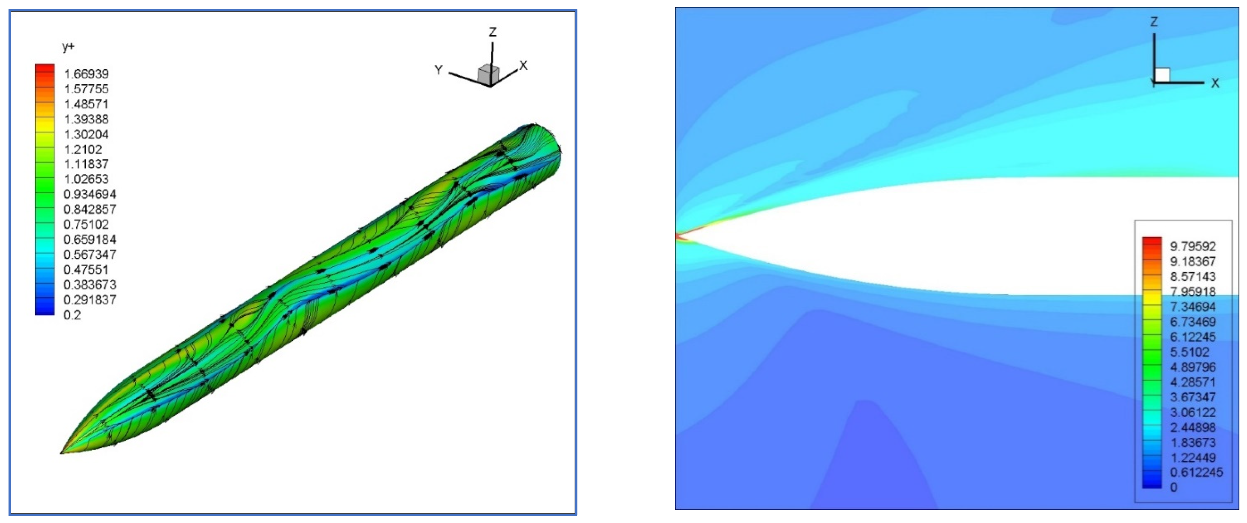
The y⁺ values in the first cells close to the body were of order 1, as well as the CFL number, except in the tip region. Figure 4 shows contours of y⁺ values at the body surface (left figure) and contours of CFL number in the tip region at the plane y = 0 (right figure) for the structured grid solution using the standard time step (Δt = 5 × 10⁻⁴ s). In another paper of the authors, the influence of the turbulence models employed is analyzed comparing the theoretical solutions with the experimental data [17]. This validation at angle of attack 45 degrees gave confidence in the theoretical method employed and in the size and density of the meshes used for the calculations.

5. Global and Convective Instabilities: Roughness Effect

The validation process was done basically with the structured grid, but also many calculations were carried out with the reference unstructured grid. The angle of attack chosen—45 degrees—was large, such that the flow was asymmetric. According with experimental studies, the angle of attack for onset of asymmetry is related with the nose angle. For ogives, cones and other short bodies this angle is: ${\alpha }_{onset}=2\cdot {\delta }_n$ [4]. This value is reduced as the fineness ratio increases [1], indicating an instability due to the afterbody. And this is valid for smooth models. For our model, using this expression, and taking into account that the nose angles is ${\delta }_n=18.92\hspace{0.17em}\mathrm{deg}.$ the angle of attack for onset is ${\alpha }_{onset}\approx 37.84\hspace{0.17em}\mathrm{deg}.$

Therefore, the body flies at the range of angles of attack where the flow is asymmetric. The origin of this asymmetry was established by several authors as a global instability of the flow: a very small perturbation of the free flow will lead the flow to depart from an unstable symmetric solution to a bi-stable asymmetric solution [1,8,18].

On the other hand, the orientation angle dependence observed in the side and normal forces lies on the result of the addition of an asymmetric flow due to a convective (spatial) instability produced for geometric random irregularities. Roughness plays a very important role in triggering these instabilities [1,7,8,18].

As the reference structured grid was theoretically a grid with a very low numerical roughness (see Section 3) and the reference unstructured grid resembles a ‘rough’ model, two studies varying the orientation angle at the angle of attack 45 degrees were carried out, using both the reference structured and unstructured grids.

5.1. Global Instability: Structured Grid

Calculations at several azimuth or orientation angles at the same angle of attack were done. The orientation angle is defined counterclockwise from the point defined at plane y = 0 at the lowest z-coordinate. These angles were Φ = 0, 45, 90, 135, 180, 225, 270, 315 and 360 degrees. Two type of calculations were done.

The first type of calculations were done using the following procedure: a steady calculation with a very large number of iterations was done, and then, transient computations within a period of T = 2 s were carried out using as initial flow field that obtained in the previous steady calculations. Using this method, most of the solutions obtained absolute values of the side force very similar, although not exactly equal. Most of them led to negative side forces, but there were a few number which obtained positive side force of similar absolute value.

The second type of calculations were done using the following procedure: transient computations within a period of T = 3 s were carried out using as initial flow field a quasi-uniform flow field (very small number of iterations done previously). The results were similar to those obtained with the first method. Again, positive or negative side force were obtained with very similar absolute vales.

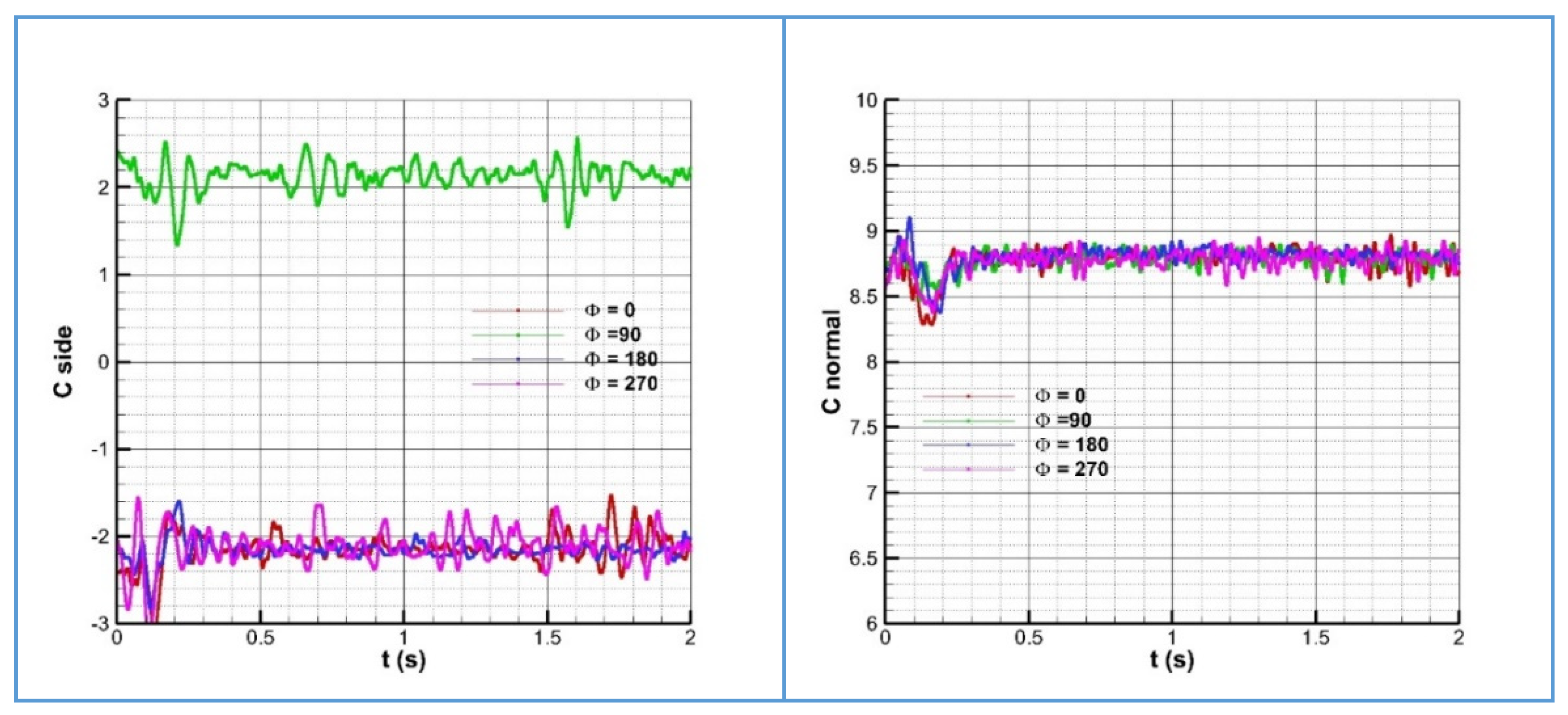
The calculations with the structured mesh at different orientation angles showed a similar side force in magnitude; but in some cases the sign differed. This is plotted in Figure 5. The solution for orientation angle Φ = 90 degrees is positive, while for the other angles the negative solution is obtained. The initial conditions or initial perturbations may be the cause for the solution to achieve one of the two possible solutions. It has been checked that at the same orientation angle the negative and positive solutions are obtained, using only different initial steady solutions. Therefore, the results obtained with the structured grid, which has a very low numerical roughness, seem to be in consonance with the experimental solutions, which at high angle of attack reproduce a bi-stable pattern of the side force, and a similar normal force, not dependent in magnitude on the orientation angle.

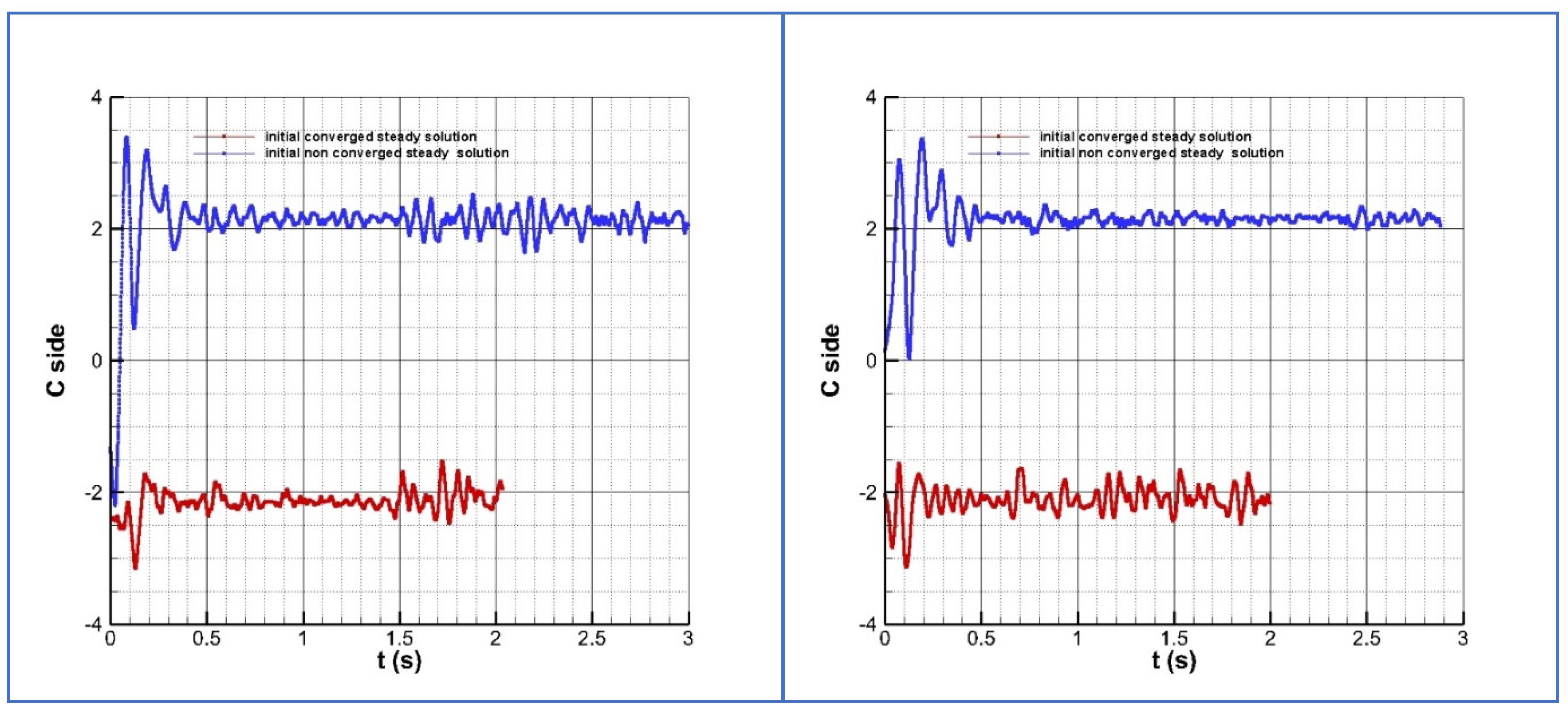
It is interesting to compare the solutions at two orientation angles: Φ = 0 degrees and Φ = 270 degrees. The side force coefficients at these two angles of orientation at two different initial conditions are plotted in Figure 6. The solution in red indicates the side force coefficient history with an initial flow field obtained from a steady calculation, while the blue line indicates an initial quasi-uniform flow field. It can be seen for the angle Φ = 0 degrees that both initial side forces are negative, but there is a jump in the second method to a positive side force, while the side force keeps its negative sign when using the steady flow solution as initial flow field. For the orientation angle Φ = 270 deg. it is worth noting that the absolute value of the side force at the beginning of the procedure for the second method case, is not equal to that of the orientation angle Φ = 0; in fact closer to zero as an initial uniform flow field can produce. For this angle, both the negative and positive side force solutions are also obtained. The differences in both cases are the initial conditions. The rest of numerical parameters, methods, grids, etc. was kept.

The main conclusion obtained from all these calculations at several orientation angles was that initial perturbations coming from a different initial flow field, but also random numerical perturbations which can produce some bias in the numerical method are sufficient to lead to a positive or negative side force solution, but both solutions are qualitative and quantitative very similar, being one solution the mirror solution of the other. Therefore, there is a numerical mechanism which is capable to drive the process to achieve a bi-stable pattern of the flow field. The influence of roughness is very small, as the grid is basically axisymmetric. Therefore, the orientation angle effects are of minor influence.

5.2. Convective Instability: Unstructured Grid

The unstructured grid was shown in the Section 3 to resemble a rough model. The averaged numerical roughness at the cylinder part was r_n/D = 40–60 × 10⁻⁶ and larger at the ogive.

A similar procedure calculating at the same angle of attack (α = 45 degrees) and different orientation angles was carried out.

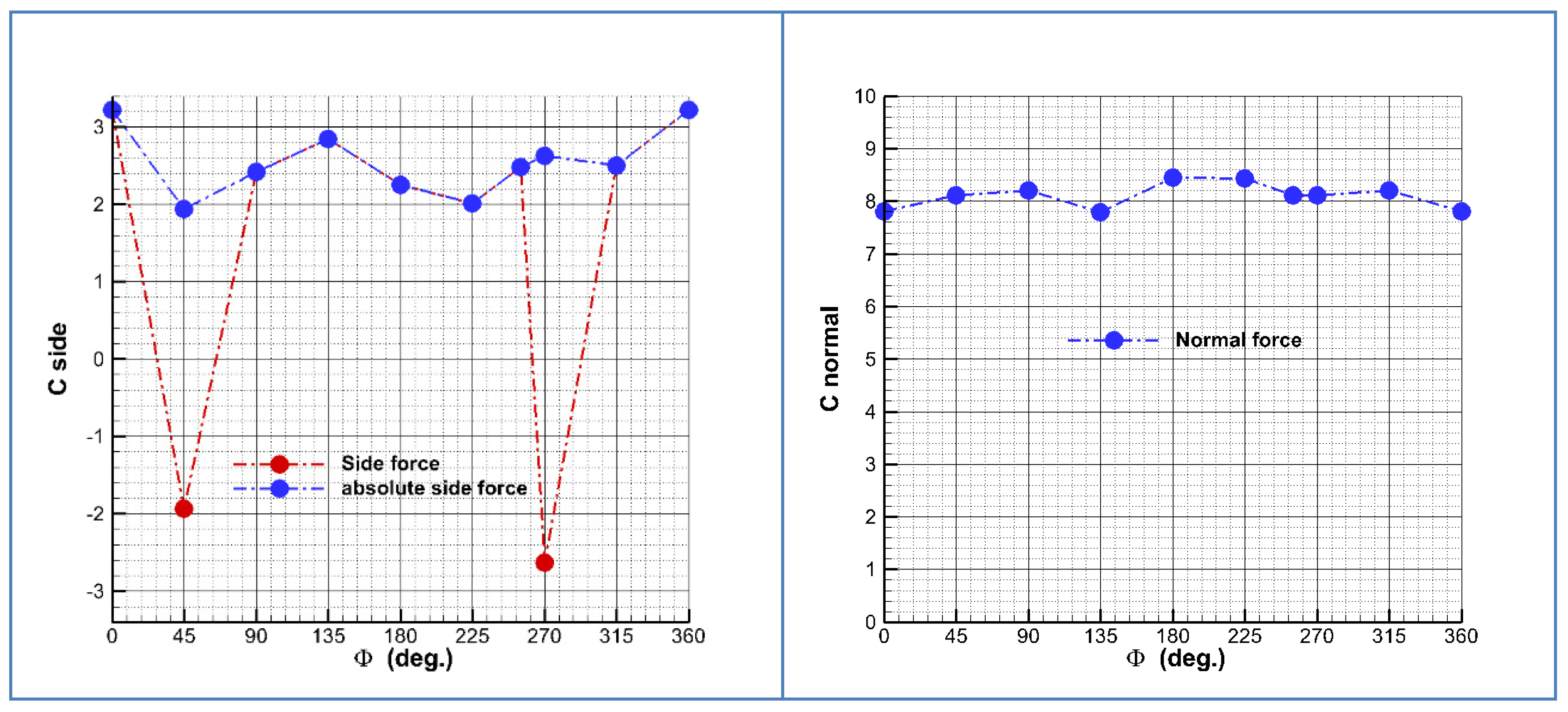
The results of averaged side and normal force coefficient for eight orientation angles within a period of T = 0.1 s are shown in

Table 1. Side and normal force coefficients versus orientation angle for the case at Ma = 0.2, Re = 2 × 10⁶, α = 45 deg. Unstructured and structured grids.

Φ (deg.)	CY	CN
0	3.22 ± 0.35	7.80 ± 0.12
45	−1.94 ± 0.57	8.11 ± 0.22
90	2.42 ± 0.50	8.20 ± 0.15
135	2.87 ± 0.45	7.79 ± 0.11
180	2.19 ± 0.52	8.42 ± 0.18
225	2.01 ± 0.60	8.44 ± 0.17
270	−2.63 ± 0.48	8.12 ± 0.16
315	2.50 ± 0.52	8.21 ± 0.16
Structured	2.99 ± 0.27	7.77 ± 0.10
Experimental	−3.37	9.22

compared to the structured grid solution–independent of the orientation angle–and to the experimental data obtained from reference [10]. There are two orientation angles for which the side force is negative. In one case (Φ = 270 deg.), the initial condition (steady solution) was of similar sign, while in the other case (Φ = 45 deg.) there was a change of sign for the specular final solution respect to the initial condition.

Due to the influence of the initial condition to end up with a positive or negative side force, the sign of the side force in Table 1 is of little relevance, but it is important to observe the large differences induced by the orientation angle on the absolute values of C_Y in the case of an unstructured mesh (that is, for an axisymmetric body with a rough surface and a non-symmetric grid).

The global (averaged values in a period of 0.1 s) side and normal force coefficients are plotted versus the orientation angle in Figure 7. Regarding the side force, the absolute value is also plotted with the orientation angle. This value is ranging within the levels of 1.94 to 3.22. There is an important change in the value, showing a strong dependence of the side force with the orientation angle. This is an effect of the convective instability. Regarding the normal force, the variation with the orientation angle is small but significant anyway.

The normal force coefficient shows small variations, with a minimum value of 7.79 and a maximum of 8.44. Regarding the average value (8.13) there is a variation of 8%. And the average value is 5% larger than that of the structured mesh. But, the side force coefficient ranges from a minimum averaged value of 1.94 to a maximum of 3.22, very close to the experimental value. These are variations of 50 %. It is worth noting that experimental data corresponding to several tests (see Refs. [1,4]) show variations up to 100% in this side force. The maximum value of side force is approximately 7% larger than that obtained with the structured mesh (2.99). Then, a trend of an increment of the side and normal force coefficients values of 5–7% is obtained in these numerical simulations. But, the oscillation of the side force is larger than that of the normal force. This may be the effect of the convective instability due to the geometrical imperfections simulated. Surface roughness increases then the lateral and normal forces on this kind of axisymmetric and elongated bodies.

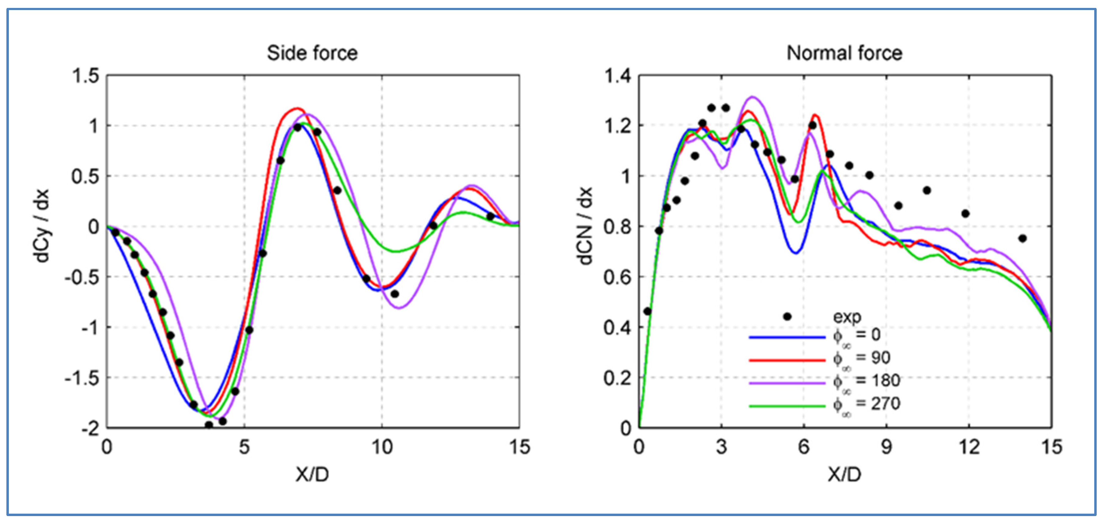
The discrete averages of both the side and normal force coefficients calculated in the last 0.1 s, are represented in the Figure 8. The experimental data are also represented for comparison. As the experimental data show negative side force (see Table 1), the negative theoretical solutions are compared with these data.

There are important differences between each theoretical solution in the slope of the local side force coefficient at the tip nose region. A convective instability due to small imperfections or irregularities is the mechanism that some authors consider to explain the large side force variations [1,3,4,8]. This mechanism should add to the global instability (hydrodynamic instability) remarked by Champigny [1], Keener and Chapman [3] and Bridges [8]. The irregularities of the surface unstructured mesh are large enough to have a strong influence in the flow structure.

Then, it is concluded that the type of grid has a decisive role in the numerical simulations. A structured axisymmetric grid resembles a very smooth body and the appearance of an asymmetric flow is due to a hydrodynamic (global or temporal) instability [1,18]. There is a bi-stable solution with two specular but otherwise similar flow field structures. However, a grid with large enough irregularities to resemble a rough model achieves different solutions. In this case, the side and normal forces are orientation angle dependent, as the surface mesh is simulating a body with irregularly distributed roughness.

The decreasing trend of the experimental normal force in the cylindrical zone is well captured by the numerical solutions, although at a lower level (see the right side of Figure 8), likely due to an excessive dissipation of the vortices. The global normal forces are clearly below the experimental values, as can be seen in Table 1. The computations match even better the trend of the experimental side force (Figure 8, left side). However, since the overall side force is the balance between the positive and negative areas of a sinusoid, slight differences in the local force can lead to remarkable deviations in the integral value, such as those of C_Y in Table 1.

6. Conclusions

The flow at high angles of attack over axisymmetric configurations is not symmetric. The mechanism that triggers the asymmetry may be a combination of a global or hydrodynamic instability (temporal instability) combined with a convective instability (spatial instability) due to microscopic irregularities of the configuration. In order to study theoretically this phenomenon, numerical simulations with the Unsteady Reynolds Averaged Navier-Stokes equations (URANS) have been conducted for an ogive-cylinder configuration at low subsonic flow and high angle of attack. For the numerical prediction of the flow about a missile type configuration, an assessment of the effect of structured and unstructured meshes is very important. How the body surface is modelled is very relevant; especially the tip zone of the body. Either configuration resembles a smooth or a rough model. The analysis has led to the conclusion that the mechanisms of global (temporal) and convective (spatial) instabilities are present in the rough model configuration (unstructured grid for the theoretical calculations) producing an orientation angle effect. While for the smooth model, which is modelled with a structured grid for the theoretical computations, there is only a global instability mechanism due to a small perturbations of the flow, which leads to an asymmetric flow at large angles of attack. Regarding the side force, there is a bi-stable pattern solution, one mirror of each other.