Investigation of a Hybrid LSTM + 1DCNN Approach to Predict In-Cylinder Pressure of Internal Combustion Engines

Abstract

The control of internal combustion engines is becoming increasingly challenging to the customer’s requirements for growing performance and ever-stringent emission regulations. Therefore, significant computational efforts are required to manage the large amount of data coming from the field for engine optimization, leading to increased operating times and costs. Machine-learning techniques are being increasingly used in the automotive field as virtual sensors, fault detection systems, and performance-optimization applications for their real-time and low-cost implementation. Among them, the combination of long short-term memory (LSTM) together with one-dimensional convolutional neural networks (1DCNN), i.e., LSTM + 1DCNN, has proved to be a promising tool for signal analysis. The architecture exploits the CNN characteristic to combine feature classification and extraction, creating a single adaptive learning body with the ability of LSTM to follow the sequential nature of sensor measurements over time. The current research focus is on evaluating the possibility of integrating virtual sensors into the on-board control system. Specifically, the primary objective is to assess and harness the potential of advanced machine-learning technologies to replace physical sensors. In realizing this goal, the present work establishes the first step by evaluating the forecasting performance of a LSTM + 1DCNN architecture. Experimental data coming from a three-cylinder spark-ignition engine under different operating conditions are used to predict the engine’s in-cylinder pressure traces. Since using in-cylinder pressure transducers in road cars is not economically viable, adopting advanced machine-learning technologies becomes crucial to avoid structural modifications while preserving engine integrity. The results show that LSTM + 1DCNN is particularly suited for the prediction of signals characterized by a higher variability. In particular, it consistently outperforms other architectures utilized for comparative purposes, achieving average error percentages below 2%. As cycle-to-cycle variability increases, LSTM + 1DCNN reaches average error percentages below 1.5%, demonstrating the architecture’s potential for replacing physical sensors.

1. Introduction

Internal combustion engine testing is becoming increasingly difficult because of increasingly stringent regulations on pollutant emissions [1,2,3] and increasing performance demands from customers [4,5,6]. Hence, exploring modern combustion strategies such as low-temperature combustions [7,8], expanding the use of renewable fuels [9], and increasing the hybridization level of vehicles are mandatory to meet the demands of sustainable mobility [10,11]. Concerning modern spark-ignition (SI) engines, the path to reduce fuel consumption demands the adoption of high boost levels in conjunction with downsizing [12,13], as well as water injection [14,15] and lean and/or exhaust gas recirculation diluted mixtures [16,17,18]. As a result, the engine complexity increases [19,20], and therefore data analysis tools need to handle large amounts of data from various physical sensors during engine calibration and runtime operations [21,22,23]. Improving engine performance requires significant computational efforts [24,25], which results in longer operating times and higher costs [26]. As a result, automotive researchers aim to discover cutting-edge technologies that can effectively monitor engine parameters [27,28,29] to improve performance while lowering consumption, pollutant emissions, and operating longevity [30,31]. Machine-learning (ML) techniques are becoming more prevalent in automotive applications due to their real-time capabilities, low-cost hardware implementation, and compact setup. These techniques are used for virtual sensors [32,33], fault detection systems [34], and performance optimization [35]. By using interpolation-based techniques, they can predict parameters and reduce the need for evaluating multiple operating points. This leads to significant improvements in memory and computational speed [36,37,38,39,40,41,42,43,44,45,46]. Based on the different ML approaches available, the LSTM + 1DCNN method appears to be a reliable way to conduct signal analysis. LSTM, which stands for long short-term memory, is a type of recurrent neural network (RNN) [47] that can effectively handle long-term relationships using ‘gates’ located in each cell. This is because it can model the sequential nature of sensor measurements over time [42,43]. Shin et al. [44] employed a long short-term memory approach to predict soot emissions from a diesel engine during dynamic conditions, specifically the worldwide harmonized light vehicles test procedure cycles. They compared its performance to that of a deep neural network (DNN). The LSTM model demonstrated a higher accuracy, with an R² value of 0.9761, in contrast to the DNN model, which achieved an R² value of 0.9215. The LSTM model’s predictions showed mean absolute errors (MAEs) ranging from 0.30% to 1.47% when compared to the maximum measured values in the transient cycles. Remarkably, the LSTM model excelled in capturing local data variations and peak values.

Norouzi et al. [45] utilized a deep recurrent neural network with LSTM layers to develop a model for predicting the emissions and performance of a 4.5-L four-cylinder Cummins diesel engine in an industrial setting. They subsequently used this model for implementing a nonlinear model predictive controller (NMPC). The LSTM achieved higher R² values of 0.9761 compared to a DNN (R² = 0.9215) used for comparison and closely matched the NMPC performance, achieving NOx reductions of up to 63.4% (at 1200 rpm). Importantly, LSTM-based controllers significantly reduced the computational time compared to conventional controllers while maintaining performance.

One-dimensional convolutional neural networks (1D-CNN) have been proposed for various applications, such as data classification, early diagnosis, structural health monitoring, anomaly detection, and detecting defects in electrical motors [48,49]. The 1D-CNNs have a simple and compact architecture that performs only scalar multiplications and additions during real-time 1D convolutions. This results in significant time savings and allows for low-cost hardware implementation, as noted in reference [50]. CNNs, or convolutional neural networks, are widely utilized due to their ability to combine feature extraction and classification in a single adaptive learning system. Fukuoka et al. [51] predicted the wind speed of Tokushima city using a mixed 1D-CNN LSTM structure. Wind speed is usually measured over a period, so the proposed method uses historical data to make current predictions. Rosato et al. [52] developed a novel deep learning approach that integrates long short-term memory networks and convolutional neural networks to tackle the challenge of predicting energy time series for a real-world solar power plant. After evaluation, it was found that the suggested framework is a practical and durable option for forecasting applications. Its significant advantage is that it uses efficient and intelligent approaches to benefit from diverse physical data sources. Our research group, referenced as [33], developed a hybrid structure using LSTM and 1DCNN to explore the feasibility of replacing a physical sensor, such as a torque meter, with a virtual one. The successful execution of this objective could have significant cost-saving benefits and prevent damage to the test bench components caused by the resonance phenomenon, as noted in references [53,54]. The structure accurately replicates the natural frequency of the recorded signal, ensuring that the absolute difference between the predicted and recorded values always remains below the acceptable threshold of 10%.

Considering ICE, the accurate analysis and prediction of engine performance parameters are crucial for optimizing fuel efficiency, reducing emissions, and improving overall reliability. Time-series data collected from sensors and engine control systems provide valuable insights into engine behavior and can be leveraged to enhance engine performance.

In this context, an ML approach was used in the present work to predict in-cylinder pressure traces of an SI engine with the aim of determining if such a method can replace physical sensors. In road cars, the use of an in-cylinder pressure transducer results in the approach not being economically viable. Using machine-learning technology can be essential in preserving engine integrity without the need for structural modifications [36]. Murugesan et al. [37] investigated the capability of an ANN approach with an integrated back propagation (BP) algorithm in predicting the in-cylinder pressure of a single-cylinder Greaves GL-400. The ANN model’s predictive capabilities, including its performance in both interpolation and extrapolation scenarios, and its robustness, are thoroughly examined through a range of error and performance analyses. Based on the error analysis conducted, the constructed ANN model demonstrates exceptional accuracy in predicting experimental outcomes, boasting a correlation coefficient close to the unit value and a mean squared error of 0.0012. A study by Jane Robert et al. [38] introduces a pioneering approach to achieving near-real-time predictions of in-cylinder engine parameters, with a strong emphasis on enhancing energy efficiency within systems. Notably, this method relies on MATLAB/Simulink, diverging from conventional practices that often demand extensive pre-characterized datasets. The research results underscore the system’s adaptability to fluctuating operational conditions, offering the potential for significant advantages over the prevalent look-up table approximations commonly used in advanced vehicle and engine control strategy development. This innovative implementation significantly enhances our capacity to optimize engine performance while minimizing data-intensive requirements, thus advancing energy management within complex systems.

Mariani et al. [39] used extreme learning machines (ELM) to simulate a spark-ignition engine’s cyclic behavior on octane fuel. Experimental runs at various speeds and crankshaft angles yielded a mean effective pressure reflecting cyclic variability (average over 100 cycles). ELM models achieved rapid predictions, surpassing iterative mathematical models. The optimized ELM models accurately approximated the mean effective pressure, consistent with experimental data.

The LSTM + 1DCNN approach utilized in the present work to predict the engine’s internal pressure was trained and evaluated utilizing experimental data obtained from a port fuel injection (PFI) three-cylinder spark-ignition (SI) engine operating under various conditions. CNN-LSTM networks offer a unique advantage by combining the local feature extraction capabilities of convolutional neural networks (CNNs) with the sequential memory modeling of long short-term memory (LSTM) networks. This fusion allows them to effectively capture spatial and temporal patterns in data, making them ideal for tasks like spatiotemporal forecasting, outperforming other AI approaches in scenarios where both spatial and temporal information are crucial [40].

The signals were acquired via a fast-combustion analysis system. Three operating points characterized by different cycle-to-cycle variabilities have been considered and the LSTM + 1DCNN performance compared with other three different artificial structures, i.e., back propagation and LSTM, to compare the advantages brought by the proposed model. The optimized structure exploited the capability of LSTM to capture long-term dependencies and temporal patterns with the ability of 1DCNN to detect patterns within smaller signal segments. The results of the present work showed that the proposed LSTM + 1DCNN architecture proved to be particularly suitable for predicting signals featuring high variability, since it is able to effectively capture and predict the target trends. The LSTM + 1DCNN enhances the performance of the other architectures tested and always achieves percentages of average error below 2%. In particular, when the cycle-to-cycle variability increases, the committed error drops below 1.5%, thus certifying the capability of the proposed algorithm to replace the task of physical sensors.

2. Materials and Methods

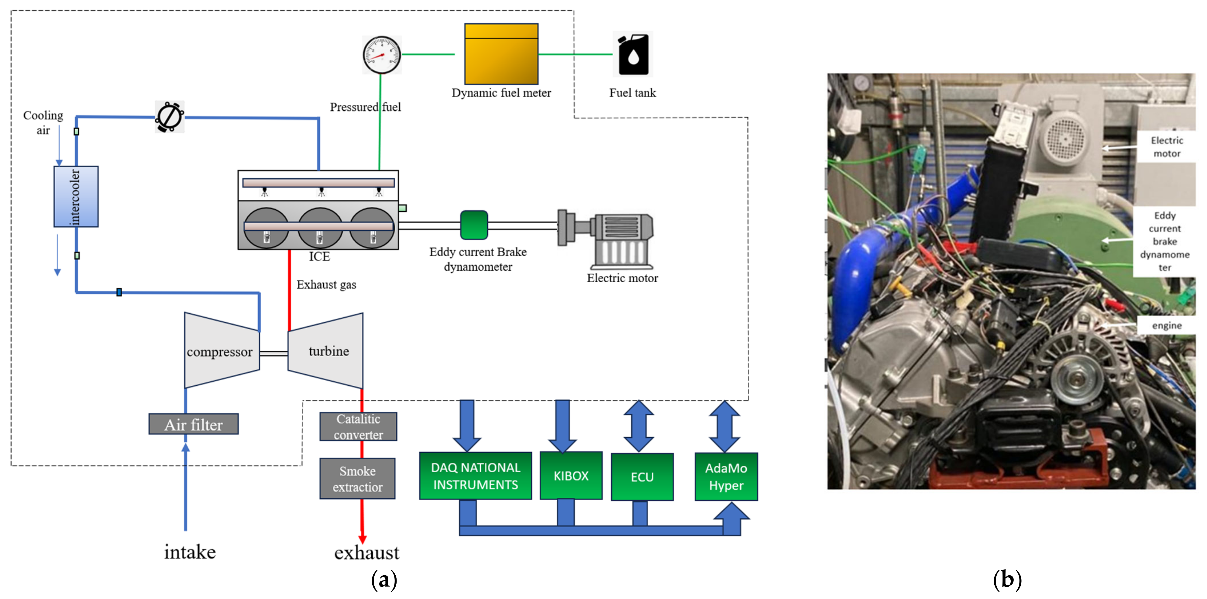
2.1. Experimental Setup

A series of tests were conducted on a 999-cc, three-cylinder engine with SMART turbocharging, 12 valves, and pent-roof combustion chambers, as indicated in

Table 1. The primary characteristics of the engine [41].

Displacement	999 cc
Cylinders	3 Cyl./4 V per Cyl.
Bore	72 mm
Stroke	81.8 mm
Compression ratio	10:1
Power	84 CV at 5250 rpm
Torque	120 Nm at 3250 rpm

[41]. The engine uses port fuel injection (PFI) technology and is designed to run on gasoline (E5) with a RON of 95 and MON of 85, which is commonly used in the European market. The gasoline is injected at a 4.2 bar absolute pressure and ignited by traditional spark-ignition systems. The use of an electric motor enables control of the engine’s speed, whether in motored or firing conditions. The engine control unit (ECU) oversees all engine parameters, while data acquisition systems from the National Instrument acquire signals from thermocouples and pressure sensors. To conduct the analysis, a Kistler KiBox combustion analysis system with a maximum temporal resolution of 0.1 CAD is used. The system collects data from various sources including the in-cylinder pressure from the piezoelectric sensor (Kistler 5018) positioned beside the flywheel, the ignition signal from ECU, the absolute crank angular position measured by an optical encoder (AVL 365C), and the pressure signals from the piezoresistive sensors (Kistler 4624A) located in the intake and exhaust ports. When the engine is running, a piezoelectric sensor measures the indicated mean effective pressure (IMEP) in the combustion chamber beside the flywheel. AdaMo Hyper was the program used to record all the related quantities. To see the layout and experimental configuration of the test bench, refer to Figure 1a,b respectively, for illustration.

2.2. Definition of the Case Study for In-Cylinder Prediction

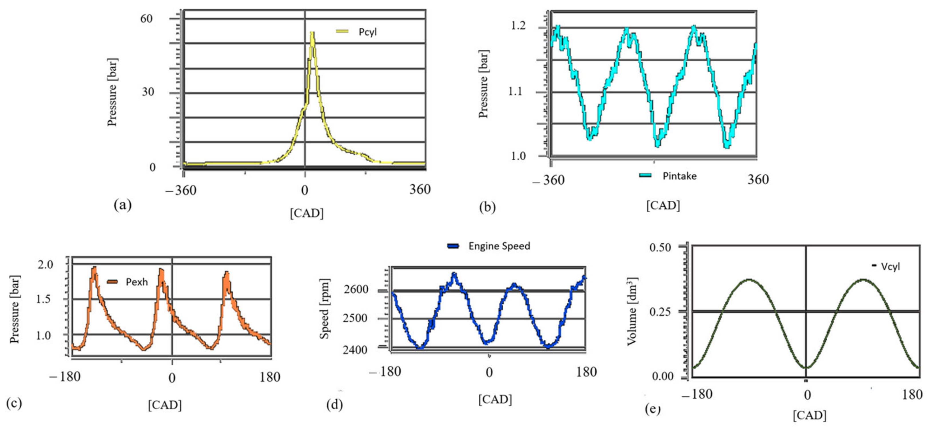
2.2.1. Definition of the Involved Parameters

The authors evaluated the performance of various algorithms in predicting the in-cylinder pressure traces of a SI engine. This was realized at three different operating points, each of which was characterized by an increasing engine speed and CoV_IMEP during full-throttle operations. The combustion stability was assessed using the coefficient of variance (CoV) of the indicated mean effective pressure (IMEP). This is the ratio of IMEP standard deviation to the IMEP mean value.

Table 2. Principal features of the operating point tested including the specific parameters measured and the corresponding values at different engine speeds.

Engine Speedavg [rpm]	IMEPavg [bar]	CoVIMEP [%]	Torqueavg [Nm]
1500	10.18	0.46	77
3250	14.15	2.13	111
2500	11.35	15.05	83

displays the average main characteristics of the tested operating points.

The KiBox analysis system continuously records with a max resolution of 0.1 CAD. All the parameters recorded by the indicating analysis system are initially selected as potential input parameters (Figure 2) to the tested architecture for forecasting the in-cylinder pressure P_cyl:

• In-cylinder volume during the engine cycle in dm³, V_cyl.
• Pressure at the intake port in bar, P_int.
• Pressure at the exhaust port in bar, P_exh.
• Position of the crankshaft during the engine cycle in the crank angle degree, CAD.
• Rotational speed of the engine in rpm, EngineSpeed.

Figure 2. Example of the acquired quantities as a function of the crank angle degree CAD. (a) In-cylinder pressure P_cyl, (b) Pressure at the intake port in bar P_int, (c) pressure at the exhaust port in bar P_exh, (d) rotational speed of the engine in rpm EngineSpeed, and (e) in-cylinder volume V_cyl.

Figure 2. Example of the acquired quantities as a function of the crank angle degree CAD. (a) In-cylinder pressure P_cyl, (b) Pressure at the intake port in bar P_int, (c) pressure at the exhaust port in bar P_exh, (d) rotational speed of the engine in rpm EngineSpeed, and (e) in-cylinder volume V_cyl.

Since not all the experimental features are recorded with the same sampling frequency, preliminary actions are realized to align the acquired data to obtain the same sampling frequency. The initial dataset of [6 × 3,614,400], corresponding to an acquisition ranging from −360 CADaTDC to 359.9 CAD aTDC, is transformed into a dataset of [6 × 67,550]. The quantities are therefore considered starting from −44.5 CAD aTDC up to 89.5 CAD aTDC with a step of 1 CAD, ensuring a comprehensive analysis of each combustion cycle focused on the complete development of the in-cylinder cylinder pressure.

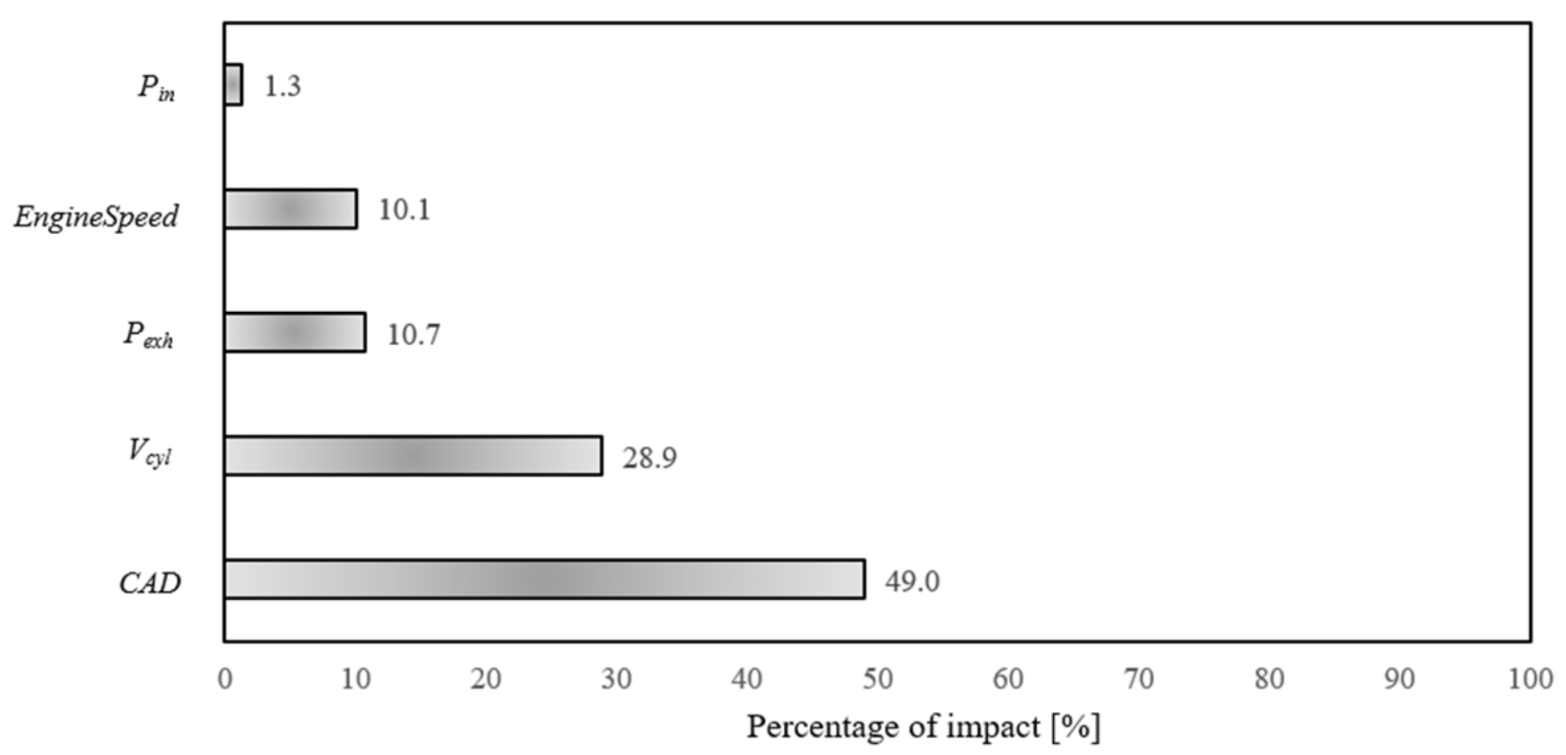
2.2.2. Evaluating the Influence of the Input Parameters on the Pressure Prediction

By eliminating parameters with low correlation, it is possible to effectively reduce the dimensions of the model and enhance its accuracy. For this reason, a preliminary analysis through the Shapley value has been performed considering the entire dataset. The objective of SHAP is to provide an explanation for the prediction of an instance by assessing the contribution of each characteristic toward the prediction. By calculating the average absolute Shapley values (ABSV), the authors were able to determine the impact of individual measured quantities on the objective function [55,56]. The results (Figure 3) show that CAD is the most influential parameter to be considered for the in-cylinder prediction, followed by the in-cylinder volume V_cyl. EngineSpeed and P_exh have a percentage of impact equal to 10% and, conversely to the pressure at the intake port, must be considered as input parameters.

To conclude, based on the analysis, P_in can be eliminated as an input feature since it has the lowest impact percentage on the P_cyl prediction. This reduces the number of inputs from 5 to 4. Previous works of the same research group [22,33] demonstrated enhancements of the performance when the architectures operate with the exclusion of the less influential parameters. Based on this, the present work shows only the architecture forecasting performance with the four input parameters previously identified (i.e., V_cyl, EngineSpeed, P_exh, and CAD). After analyzing the input parameters, a normalization process is carried out to prevent prediction errors and ensure faster convergence of the architecture. This process helps in avoiding discrepancies between input and output parameters. The values are mapped to the range [0, 1] for a better understanding. After the prediction process, the predicted data are de-normalized to offer a direct comparison with the original target experimentally acquired.

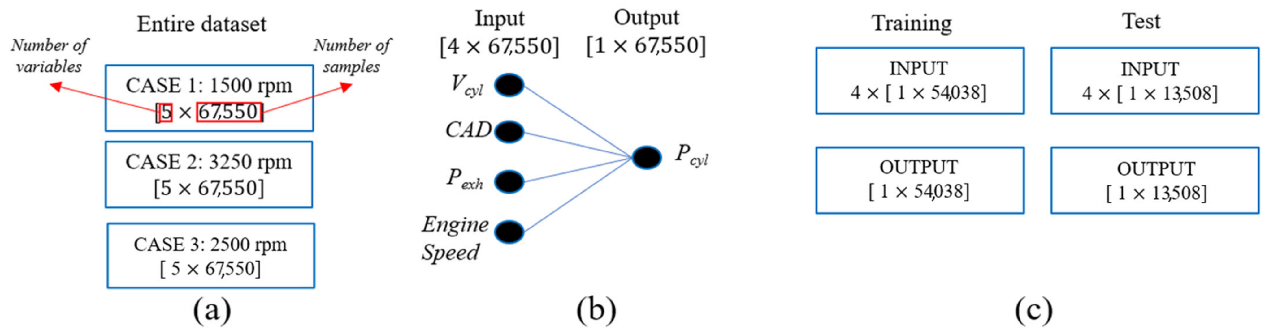
2.2.3. Definition of the Final Dataset for the Pressure Prediction

Based on the results of the sensitivity analysis, Figure 4 provides a comprehensive overview of the dataset, including the division of input and output parameters for each analyzed case. As is possible to observe, the entire dataset analyzed is composed of the three different operating points (Table 2) featured with 5 variables, each of which presenting 67,550 samples (Figure 4a). V_cyl, CAD, P_exh, and EngineSpeed [4 × 67,550] define the input parameters while the in-cylinder pressure P_cyl [1 × 67,550] is the output (Figure 4b).

In total, 80% of the data were used for the training session and the remaining 20% [4 × 13,508] during the test session to predict P_cyl [1 × 13,508] (Figure 4c). The performance of the LSTM + 1DCNN structure was compared with those of three different AI architectures on Case 1. Based on the obtained results, the other two cases, i.e., Case 2 and Case 3, were used to investigate the LSTM + 1DCNN behavior when operating with signals characterized by a higher cycle-to-cycle variability.

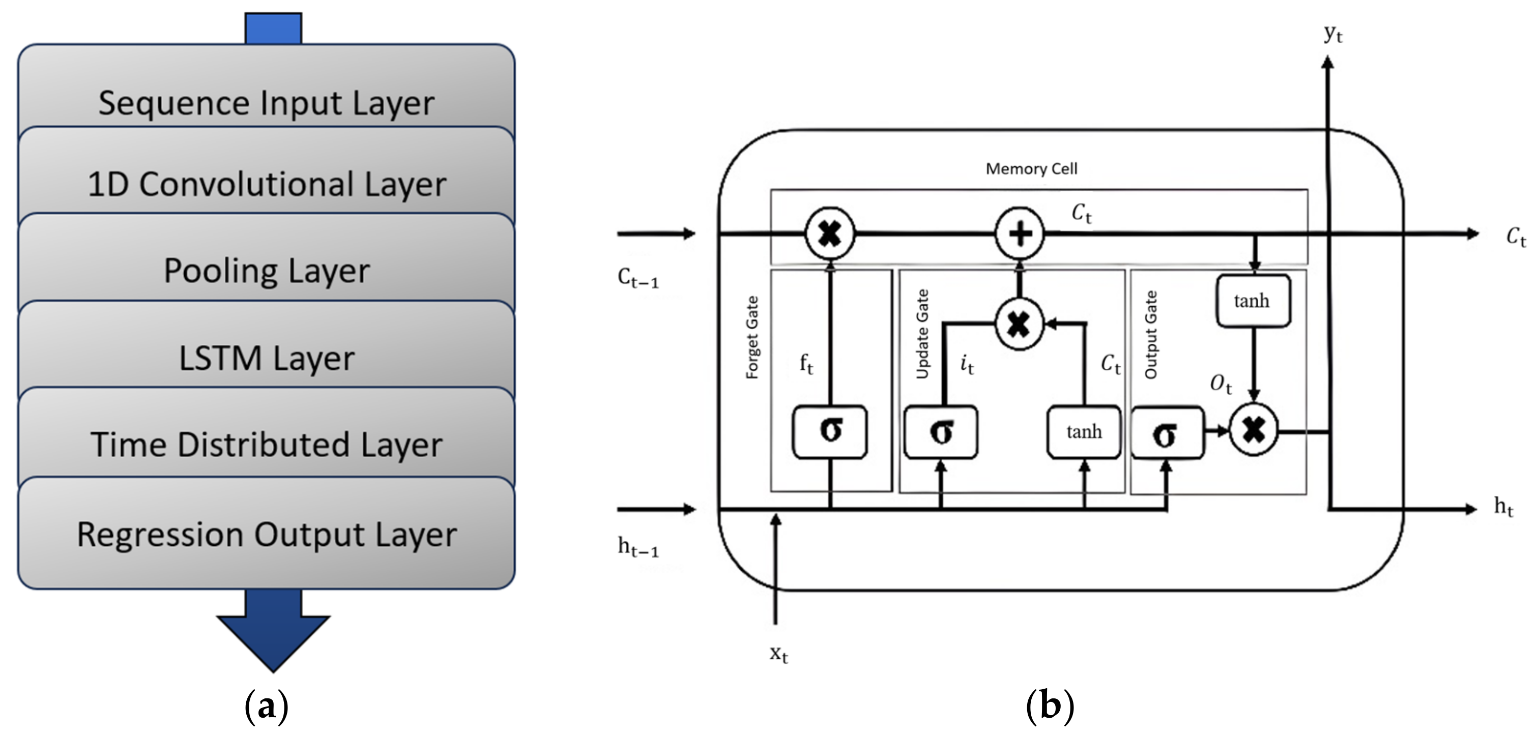
2.3. Creating an Artificial Architecture to Predict In-Cylinder Pressure

2.3.1. Structure of the LSTM + 1DCNN Model

Figure 5a displays the predictive scheme of LSTM + 1DCNN used to predict the in-cylinder pressure traces. A sequence input layer is used to pass the dataset to the network. This layer inputs sequence data into the network by establishing its size and constructing the corresponding structures. A one-dimensional CNN layer applies a 1D convolutional filter to each input frame; it is made up of neurons and a ReLu activation function. The average pooling layer calculates the average value of patches in a feature map, which helps to down-sample the maps by using the mean value in 2 × 2 cell squares. After that, another 1D convolutional level, similar to the previous one, is applied. Following this, the feature maps undergo processing by an LSTM layer consisting of hidden units. Within the LSTM network’s internal architecture (Figure 5b), gates play a crucial role. The forget gate determines which information should be kept or discarded by taking into account both the previous layer’s information (${\mathrm{h}}_{\mathrm{t}-1}$) and the current input’s information (x_t). A sigmoid function evaluates this information and generates an output between 0 and 1, indicating whether the information should be retained or not. This gate alters the previous cell state value (C_t−1). The input gate is responsible for choosing which information should be stored in the cell state. It does this in a few steps. First, a layer called the “input port layer” applies a sigmoid function (represented by σ) to decide which values should be updated. Then, a new set of candidate values (represented by a vector called C_t) is generated using a hyperbolic tangent function (represented by tanh). These two sets of values are combined and updated using the ft function, which replaces the old cell state (${\mathrm{C}}_{\mathrm{t}-1}$) with the new one (C_t). Finally, the updated cell state is multiplied by the gating function (f_t). The output gate stores a filtered version of the processed data, while the sigmoid determines which parts of the cell state to output. The cell state undergoes a tanh operation to limit the values between −1 and 1, and then it is multiplied by the sigmoid gate output. This process results in only the selected parts being produced as output. LSTMs have a distinctive structure that incorporates a forget gate activation, enabling the network to promote desired behavior through frequent port updates at every stage of the learning process. Once the LSTM is complete, the time-distributed layer distributes the feature map in a temporal vector sequence, and the regression output level calculates the mean square error loss for the regression problem.

2.3.2. Definition of the Procedures to Determine the Structural Parameters of the Proposed Models

The definition of the optimal neural structures is determined through preliminary analysis considering the training sessions’ performance. To assess the effectiveness of the model parameters, a loss function is used, and, in this case, the mean square error (MSE) is the chosen function for the task (Equation (1)):

$$\mathrm{MSE}=\frac{1}{\mathrm{N}} {{\displaystyle \sum }}_{\mathrm{i}=0}^{\mathrm{N}}{\left({\mathrm{Y}}_{\mathrm{predicted}}^{\mathrm{i}}-{\mathrm{Y}}_{\exp }^{\mathrm{i}}\right)}^2$$

(1)

where N represents the number of samples, ${\mathrm{Y}}_{\mathrm{predicted}}^{\mathrm{i}}$ refers to the predicted value while ${\mathrm{Y}}_{\exp }^{\mathrm{i}}$ refers to the target value experimentally obtained.

The network’s epoch iterations are set to 100, allowing the computation of the loss function’s final value for each prediction model once the network training reaches its maximum learning iteration. For the LSTM + 1DCNN architecture, the following structural parameters have been investigated:

• The number of neurons in the 1DCNN layers N_c varies from 50 to 200.
• The number of neurons in the LSTM hidden layers N_h varies from 50 to 200.
• The batch size B_s varies from 8 to 64.
• The model depth M_d varies from 1 to 5.

The Adam optimizer is applied to facilitate the updating of the weight matrix and bias in the LSTM network model, along with an adaptive learning rate adjustment during training. The performance of the proposed structure is assessed in comparison to two other architectures: back propagation, LSTM, and NARX [22], which were optimized based on extensive preliminary analysis similar to the LSTM + 1DCNN architecture. The optimal solutions with the lowest loss function values were selected for predicting P_cyl.

3. Results and Discussions

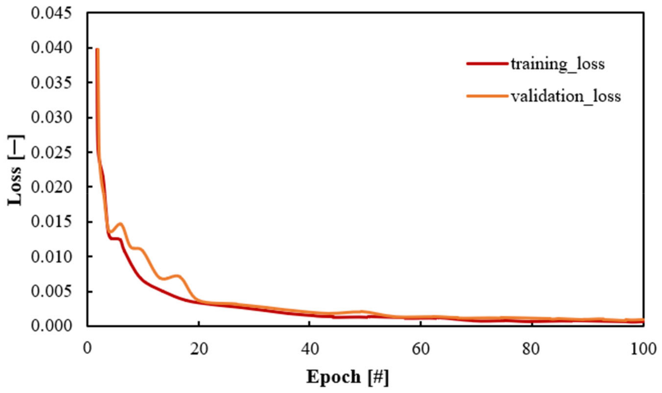
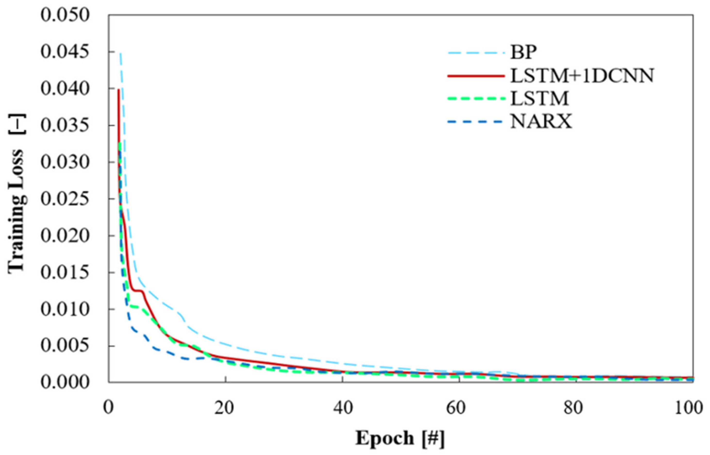
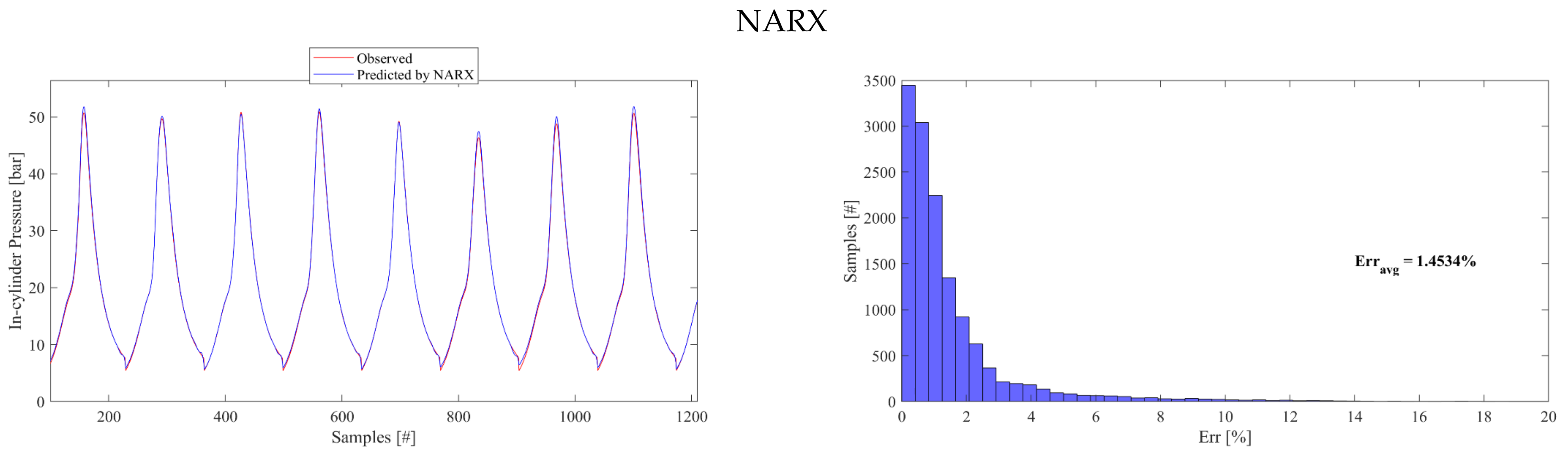
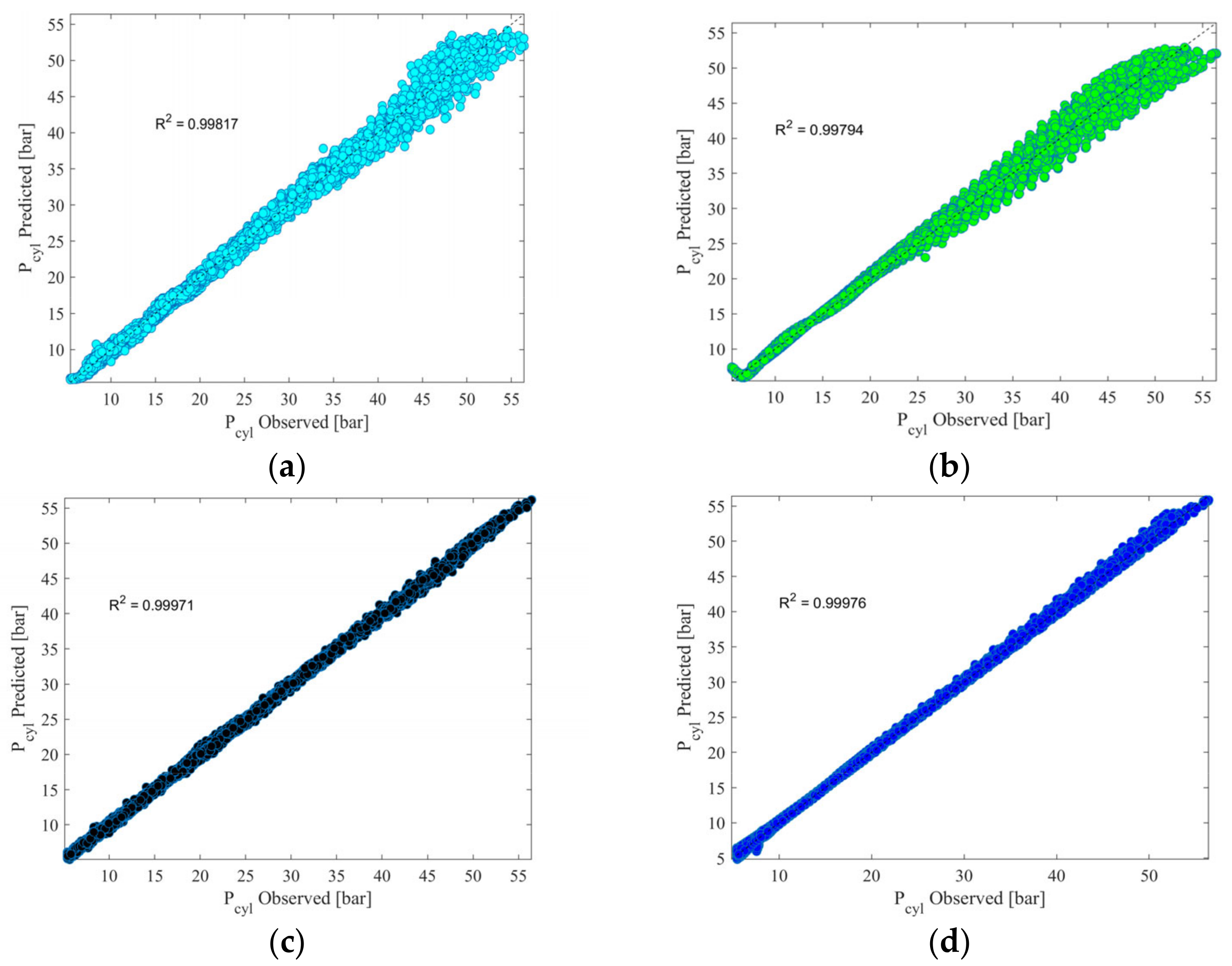
3.1. Performance on Training

Figure 6 illustrates the validation loss (val_loss) and training loss (training_loss) for the best-performing LSTM + 1DCNN configuration, i.e., N_c = 100, N_h = 150, B_s = 16, M_d = 1. The training results demonstrate that the model converges effectively without exhibiting overfitting. In the context of debugging the 1DCNN structure, it is crucial to observe that a limited number of neurons can lead to underfitting, as it may not capture sufficient features. Conversely, an excessive number can result in overfitting. Although the addition of pooling layers can mitigate overfitting, an abundance of them reduces the feature dimensions passed to the LSTM network. This reduction can hinder the LSTM’s ability to extract time-series features effectively, ultimately diminishing the network’s capacity to fit the data accurately.

To sum up, the LSTM + 1DCNN structure is composed of a one-dimensional convolutional layer with 100 neurons, a kernel size equal to three, and a ReLu activation function; a max pooling 1D layer which uses a pool size of two and a stride of two; an LSTM layer composed by 100 neurons; a time-distributed layer and a dense layer composed of one unit to perform the regression task [33].

The performance of the proposed structures is compared with three other different architectures, optimized with the same procedures as LSTM + 1DCNN, and composed as follows:

• The BP algorithm [57,58,59] consists of one input layer, and three hidden layers with each layer having 100 neurons and one output layer.
• The prediction model for the LSTM network [33] consists of an input layer, a hidden layer with 100 neurons, an output layer, and a fully connected layer.
• The NARX [22] structure is composed of [1:2] delays for each input and two hidden layers composed of 50 and 100 neurons, respectively.

Figure 7 shows the results of the first comparison between the proposed algorithms, at the operating condition of 1500 rpm and a low load, performed through the evaluation of the training losses.

In general, all trends decrease as the epoch increases, and they tend to stabilize, on average, after 50 iterations, thus indicating that the models converge without overfitting. BP reaches the stabilization zone about 20 epochs after the other architectures, while NARX presents the fastest converge speed, showing a training loss below 0.05 already at about 10 epochs. Moreover, once stabilized, it presents very low oscillations which suggests that the model could be more robust than the others at this operating point.

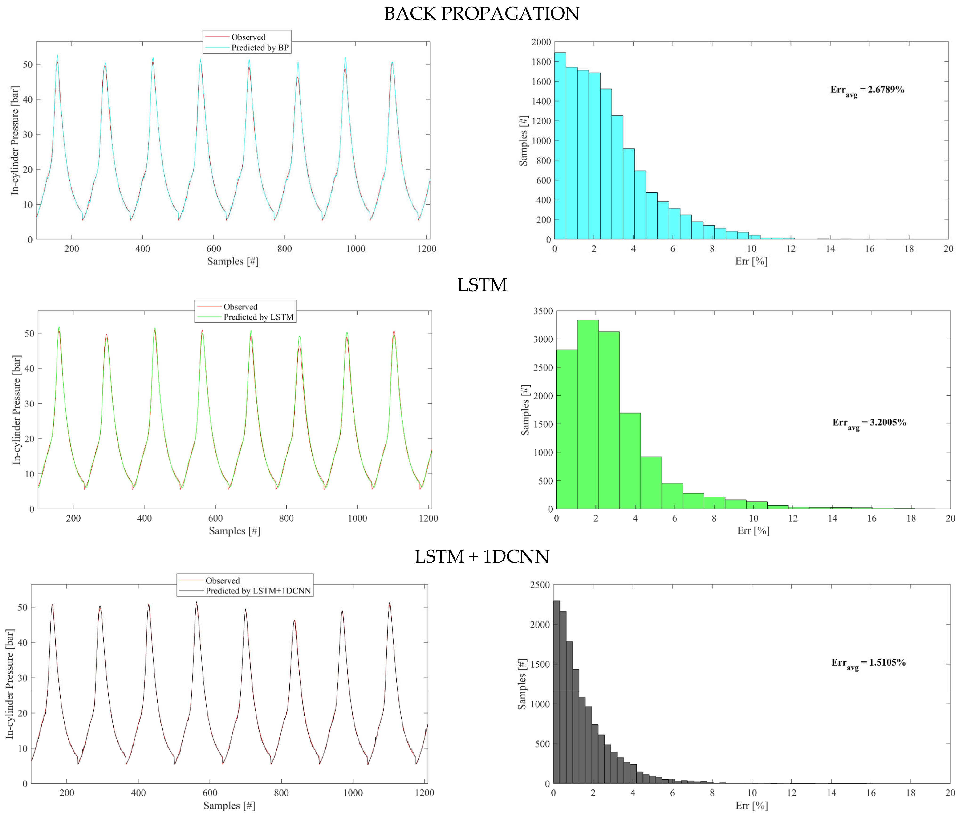
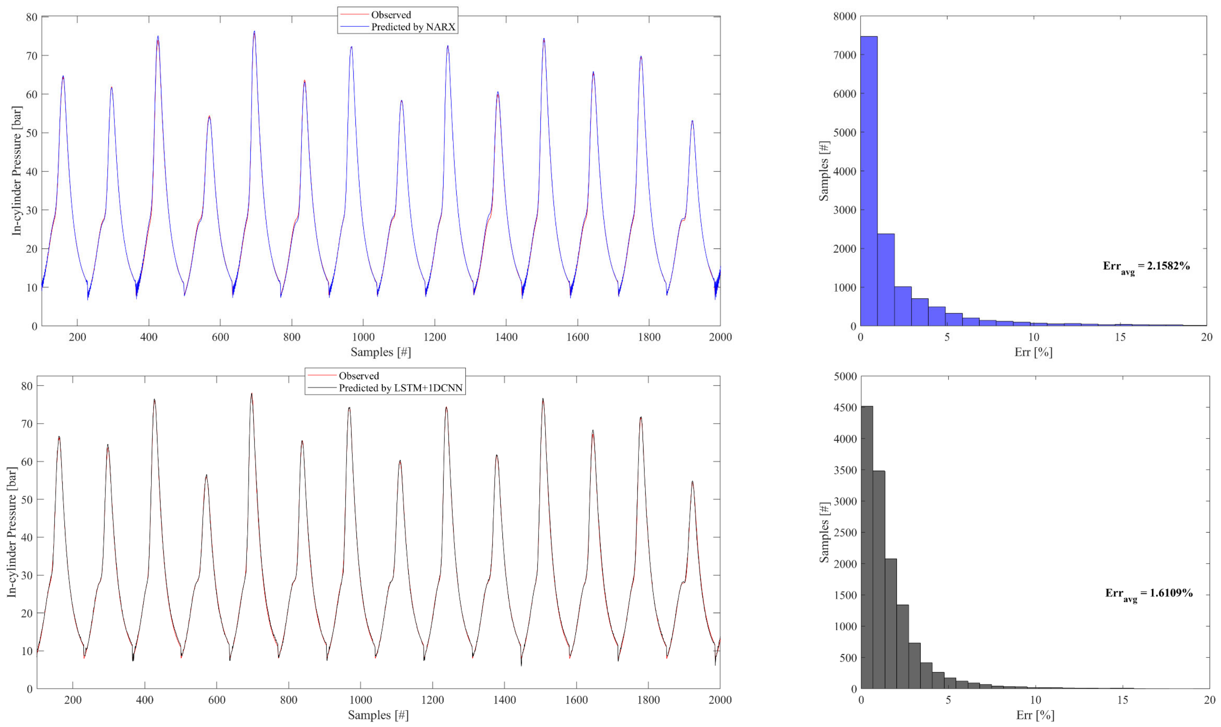
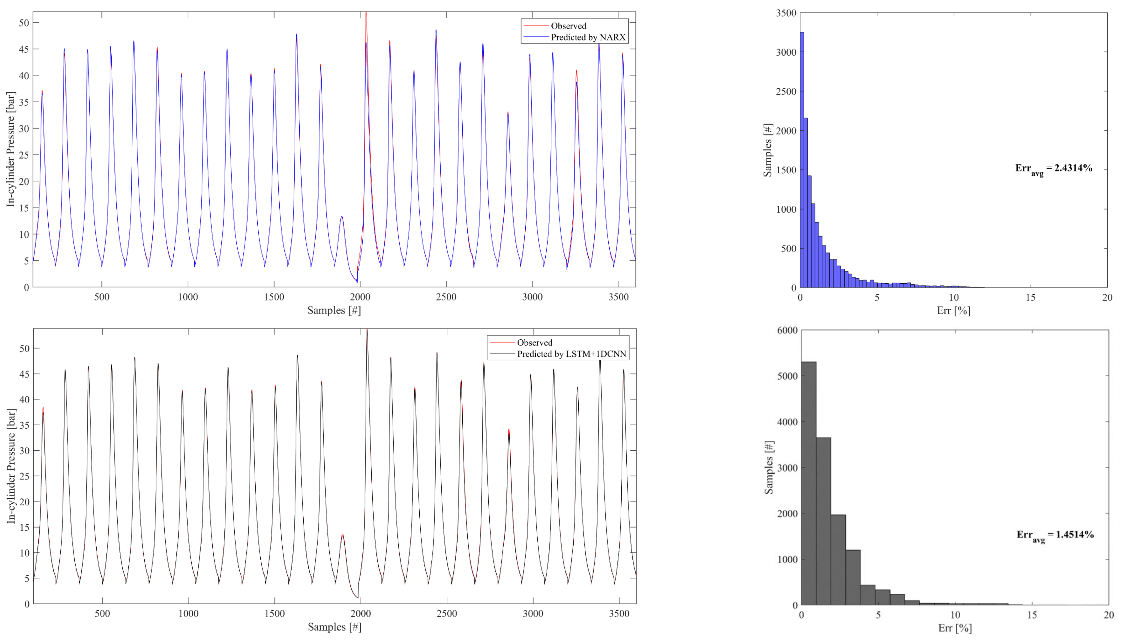
3.2. Performance on Test

Figure 8 displays the prediction of the in-cylinder pressure traces performed by each neural structure.

For the sake of clarity, since the prediction is performed on the last 100 cycles of 500, only eight events are depicted in the figure in order to better visualize the quality of the prediction.

To compare the predicted range as a whole, the deviation of each forecast’s prediction from the target across the entire range has been calculated using Equation (2).

$$\mathrm{Err}=\frac{1}{\mathrm{N}} {{\displaystyle \sum }}_{\mathrm{i}=1}^{\mathrm{N}}\frac{\left[\frac{\left|{\mathrm{Y}}_{\mathrm{predicted}}^{\mathrm{i}}-{\mathrm{Y}}_{\exp }^{\mathrm{i}}\right|}{{\mathrm{Y}}_{\exp }^{\mathrm{i}}}\right]}{\mathrm{N}}\times 100$$

(2)

In this test case, N represents the number of samples being considered and i represents the ith sample. The average percentage error, known as Err_avg, is calculated to assess the overall prediction accuracy. In order to ensure high-quality predictions, a maximum critical threshold of 10 is set for the computed errors.

All of the tested structures (Figure 8) are able to reproduce the trend of the in-cylinder pressure over time. BP shows an Err_avg below the critical threshold of 10% and equals 2.68%, with 95 samples presenting an Err over 10% corresponding to about 0.8% of the predicted samples. LSTM lowers the BP performance presenting an Err_avg equal to 3.20%, with about 3.55% of predicted samples exceeding the critical threshold of 10% corresponding to 480 samples. LSTM + 1DCNN enhances the LSTM performance showing an Err_avg of 1.51% with 10 samples exceeding a 10% error, i.e., 0.07% of the entire predicted samples. The NARX structure performs the best in terms of average errors, showing Err_avg values equal to about 1.45%, but it shows 1% of samples exceeding 10% of Err, corresponding to 139 samples. Therefore, even if the LSTM + 1DCNN error prediction is, on average, higher than the NARX one, the structure outperforms NARX in terms of the number of samples predicted with an Err below the critical threshold of 10%. The effectiveness of the two latter forecasts is also highlighted by the comparison between the observed and predicted trends, which almost overlapped with the target trend.

The accuracy of regression for each architecture tested in the prediction set is shown in Figure 9. Models show great accuracy at the lower range of analysis (i.e., low P_cyl). Increasing the in-cylinder pressure value, BP and LSTM present a higher dispersion while LSTM + 1DCNN and NARX exhibit uniform distribution across the interpolation line, without any points displaying a wide range of deviation. In particular, these architectures show the lowest dispersion degree with an R² close to the unit value. These results demonstrate that LSTM + 1DCNN and NARX possess a higher liner fitting and prediction accuracy compared to other tested architectures. The presented results highlight the robust learning capabilities of NARX and LSTM + 1DCNN structures and their ability to reproduce the target trend well.

After analyzing the results obtained, both structures (NARX and LSTM+1DCCN) were selected for the forecast activities of the other case reported in Table 2 (i.e., 3250 rpm), which is characterized by a higher variability (higher CoV_IMEP) compared to 1500 rpm. Figure 10 displays the forecasted signals against the observed signals of both architectures. Both models are able to reproduce the target trend well. NARX slightly lowers the performance compared to the previous case, showing a small increment in the percentage error up to 2.16% (compared to the 1.37% at 1500 rpm), with 545 samples exceeding 10% of the error. The LSTM + 1DCNN structure maintains a similar performance, showing an Err_avg equal to 1.61% with 0.8% of predicted samples exceeding the critical threshold of 10%.

It is clear that the LSTM + 1DCNN structure is capable of maintaining its performance when operating with signals characterized by more variability. This feature suggests that the architecture could also be suitable for predicting the in-cylinder pressure traces of unstable stationary operating points or transient cycles. For this reason, the last attempt is performed by considering an operating point characterized by CoV_IMEP = 15% (Table 2). A comparison with NARX performance is also presented to highlight the differences in the forecasting behavior. As depicted (Figure 11), NARX maintains about the same performance as the previous case (Err_avg = 2.16% at 3250 rpm) showing an Err_avg equal to 2.45% with 166 samples predicted above the critical Err threshold of 10%. The LSTM + 1DCNN structure is able to follow the signal oscillations and it gains its performance by showing an Err_avg equal to 1.43% with 89 of the predicted samples presenting an Err over the critical threshold of 10%.

4. Conclusions

The present work evaluates the forecasting performance of LSTM + 1DCNN in predicting the in-cylinder pressure traces of a three-cylinder spark-ignition engine, under different operating conditions.

The aim is to explore the potential of using advanced machine-learning technologies to replace physical sensors and evaluate the possibility of integrating virtual sensors into the on-board control system. This would eliminate the need for costly and time-consuming structural modifications. The results highlight the better quality of the LSTM + 1DCNN in reproducing the trend target signals. In comparison to the other architectures used for comparative purposes, the structure consistently shows the best performance, achieving average percentages of errors below 2%. As the variability of the engine from cycle to cycle becomes greater, the LSTM + 1DCNN is able to achieve average error percentages below 1.5%. To summarize:

• Key Findings:

The study revealed that the LSTM + 1DCNN architecture achieves convergence during training without overfitting, indicating its capacity to effectively learn from data and make precise predictions. Furthermore, when compared to other architectures the LSTM + 1DCNN consistently demonstrates a superior accuracy and robustness. These results position LSTM + 1DCNN as a promising candidate for in-cylinder prediction in spark-ignition engines.

• Implications:

These findings have significant implications for spark-ignition engine research and artificial intelligence. The development of an architecture capable of accurately predicting pressure opens opportunities for cost savings and enhanced engine performance monitoring. This innovation can lead to more efficient and dependable engine management systems. Additionally, the demonstrated robustness and accuracy of the LSTM + 1DCNN architecture makes it adaptable to various real-world engine operating conditions, potentially advancing diverse engine applications.

• Future Research and Testing:

While this study represents a substantial advancement, further research and testing are needed to validate and broaden the applicability of the LSTM + 1DCNN architecture. On-board implementation and testing under diverse operational scenarios are crucial to fully explore its potential benefits. This includes testing the architecture with larger datasets and various dynamic cycles.

In conclusion, this work presents a promising solution for replacing physical pressure sensors and contributes to the broader field of artificial intelligence in engine research. The LSTM + 1DCNN architecture’s robustness and accuracy position it as an attractive choice for enhancing engine performance monitoring, paving the way for further advancements in the field.

References

1. Lim, K.Y.H.; Zheng, P.; Chen, C.H. A state-of-the-art survey of Digital Twin: Techniques, engineering product lifecycle management and business innovation perspectives. J. Intell. Manuf. 2020, 31, 1313–1337. [Google Scholar] [CrossRef]
2. Joshi, A. Review of vehicle engine efficiency and emissions. SAE Int. J. Adv. Curr. Pract. Mobil. 2020, 2, 2479–2507. [Google Scholar] [CrossRef]
3. Reitz, R.D.; Ogawa, H.; Payri, R.; Fansler, T.; Kokjohn, S.; Moriyoshi, Y.; Agarwal, A.K.; Arcoumanis, D.; Assanis, D.; Bae, C.; et al. IJER Editorial: The Future of the Internal Combustion Engine. Int. J. Engine Res. 2020, 21, 3–10. [Google Scholar] [CrossRef]
4. Al-Samari, A. Study of emissions and fuel economy for parallel hybrid versus conventional vehicles on real world and standard driving cycles. Alex. Eng. J. 2017, 56, 721–726. [Google Scholar] [CrossRef]
5. Witanowski, Ł.; Breńkacz, Ł.; Szewczuk-Krypa, N.; Dorosińska-Komor, M.; Puchalski, B. Comparable analysis of PID controller settings in order to ensure reliable operation of active foil bearings. Eksploat. I Niezawodn. 2022, 24, 377–385. [Google Scholar] [CrossRef]
6. Rudolph, C.; Freund, D.; Kaczmarek, D.; Atakan, B. Low-calorific ammonia containing off-gas mixture: Modelling the conversion in HCCI engines. Combust. Flame 2022, 243, 112063. [Google Scholar] [CrossRef]
7. García, A.; Monsalve-Serrano, J. Analysis of a series hybrid vehicle concept that combines low temperature combustion and biofuels as power source. Results Eng. 2019, 1, 100001. [Google Scholar] [CrossRef]
8. He, X.; Wang, Q.; Fernandes, R.; Shu, B. Investigation on the autoignition characteristics of propanol and butanol isomers under diluted lean conditions for stratified low temperature combustion. Combust. Flame 2022, 237, 111818. [Google Scholar] [CrossRef]
9. Alvarez, C.E.C.; Couto, G.E.; Roso, V.R.; Thiriet, A.B.; Valle, R.M. A review of prechamber ignition systems as lean combustion technology for SI engines. Appl. Therm. Eng. 2018, 128, 107–120. [Google Scholar] [CrossRef]
10. Lukic, S.M.; Ali, E. Effects of drivetrain hybridization on fuel economy and dynamic performance of parallel hybrid electric vehicles. IEEE Trans. Veh. Technol. 2004, 53, 385–389. [Google Scholar] [CrossRef]
11. Chau, K.T.; Wong, Y.S. Hybridization of energy sources in electric vehicles. Energy Convers. Manag. 2001, 42, 1059–1069. [Google Scholar] [CrossRef]
12. Zou, R.; Liu, J.; Jiao, H.; Wang, N.; Zhao, J. Numerical study on auto-ignition development and knocking characteristics of a downsized rotary engine under different inlet pressures. Fuel 2022, 309, 122046. [Google Scholar] [CrossRef]
13. Kouhyar, F.; Nikzadfar, K. A Model-Based Investigation of Electrically Split Turbocharger Systems Capabilities to Overcome the Drawbacks of High-Boost Downsized Engines; SAE Technical Paper No. 2022-01-5052; SAE International: Warrendale, PA, USA, 2022. [Google Scholar]
14. Lanni, D.; Galloni, E.; Fontana, G. Numerical analysis of the effects of port water injection in a downsized SI engine at partial and full load operation. Appl. Therm. Eng. 2022, 205, 118060. [Google Scholar] [CrossRef]
15. Sun, X.; Ning, J.; Liang, X.; Jing, G.; Chen, Y.; Chen, G. Effect of direct water injection on combustion and emissions characteristics of marine diesel engines. Fuel 2022, 309, 122213. [Google Scholar] [CrossRef]
16. Zhou, L.; Song, Y.; Hua, J.; Liu, F.; Liu, Z.; Wei, H. Effects of different hole structures of pre-chamber with turbulent jet ignition on the flame propagation and lean combustion performance of a single-cylinder engine. Fuel 2022, 308, 121902. [Google Scholar] [CrossRef]
17. Molina, S.; Novella, R.; Gomez-Soriano, J.; Olcina-Girona, M. Experimental Evaluation of Methane-Hydrogen Mixtures for Enabling Stable Lean Combustion in Spark-Ignition Engines for Automotive Applications; SAE Technical Paper No. 2022-01-0471; SAE International: Warrendale, PA, USA, 2022. [Google Scholar]
18. Liu, X.; Aljabri, H.; Silva, M.; AlRamadan, A.S.; Ben Houidi, M.; Cenker, E.; Im, H.G. Hydrogen pre-chamber combustion at lean-burn conditions on a heavy-duty diesel engine: A computational study. Fuel 2023, 335, 127042. [Google Scholar] [CrossRef]
19. Atkinson, C. Fuel Efficiency Optimization Using Rapid Transient Engine Calibration; SAE Technical Paper No. 2014-01-2359; SAE International: Warrendale, PA, USA, 2014. [Google Scholar]
20. Dimopoulos, P.; Rechsteiner, C.; Soltic, P.; Laemmle, C.; Boulouchos, K. Increase of passenger car engine efficiency with low engine-out emissions using hydrogen–natural gas mixtures: A thermodynamic analysis. Int. J. Hydrogen Energy 2007, 32, 3073–3083. [Google Scholar] [CrossRef]
21. Iqbal, M.Y.; Wang, T.; Li, G.; Li, S.; Hu, G.; Yang, T.; Gu, F.; Al-Nehari, M. Development and Validation of a Vibration-Based Virtual Sensor for Real-Time Monitoring NOx Emissions of a Diesel Engine. Machines 2022, 10, 594. [Google Scholar] [CrossRef]
22. Ricci, F.; Petrucci, L.; Mariani, F. Using a Machine Learning Approach to Evaluate the NOx Emissions in a Spark-Ignition Optical Engine. Information 2023, 14, 224. [Google Scholar] [CrossRef]
23. Hasan, A.; Leung, P.; Tsolakis, A.; Golunski, S.; Xu, H.; Wyszynski, M.; Richardson, S. Effect of composite aftertreatment catalyst on alkane, alkene and monocyclic aromatic emissions from an HCCI/SI gasoline engine. Fuel 2011, 90, 1457–1464. [Google Scholar] [CrossRef]
24. Zembi, J.; Ricci, F.; Grimaldi, C.; Battistoni, M. Numerical Simulation of the Early Flame Development Produced by a Barrier Discharge Igniter in an Optical Access Engine; SAE Technical Paper No. 2021-24-0011; SAE International: Warrendale, PA, USA, 2021. [Google Scholar]
25. Thompson, G.J.; Atkinson, C.M.; Clark, N.N.; Long, T.W.; Hanzevack, E. Neural network modelling of the emissions and performance of a heavy-duty diesel engine. Proc. Inst. Mech. Eng. Part D J. Automob. Eng. 2000, 214, 111–126. [Google Scholar] [CrossRef]
26. Escobar, C.A.; Morales-Menendez, R. Machine learning techniques for quality control in high conformance manufacturing environment. Adv. Mech. Eng. 2018, 10, 1687814018755519. [Google Scholar] [CrossRef]
27. Suzuki, K. (Ed.) Artificial Neural Networks—Industrial and Control Engineering; IntechOpen: Rijeka, Croatia, 2011. [Google Scholar]
28. Das, A.K.; Padhi, M.R.; Hansdah, D.; Panda, A.K. Optimization of engine parameters and ethanol fuel additive of a diesel engine fuelled with waste plastic oil blended diesel. Process Integr. Optim. Sustain. 2020, 4, 465–479. [Google Scholar] [CrossRef]
29. Shamekhi, A.; Shamekhi, A.H. Expert Systems with Applications: A New Approach in Improvement of Mean Value Models for Spark Ignition Engines Using Neural Networks. Expert Syst. Appl. 2015, 42, 5192–5218. [Google Scholar] [CrossRef]
30. Li, X.-Q.; Song, L.-K.; Choy, Y.-S.; Bai, G.-C. Multivariate ensembles-based hierarchical linkage strategy for system reliability evaluation of aeroengine cooling blades. Aerosp. Sci. Technol. 2023, 138, 108325. [Google Scholar] [CrossRef]
31. Li, X.-Q.; Song, L.-K.; Bai, G.-C.; Li, D.-G. Physics-informed distributed modeling for CCF reliability evaluation of aeroengine rotor systems. Int. J. Fatigue 2023, 167, 107342. [Google Scholar] [CrossRef]
32. Bai, S.; Li, M.; Lu, Q.; Fu, J.; Li, J.; Qin, L. A new measuring method of dredging concentration based on hybrid ensemble deep learning technique. Measurement 2022, 188, 110423. [Google Scholar] [CrossRef]
33. Petrucci, L.; Ricci, F.; Mariani, F.; Mariani, A. From real to virtual sensors, an artificial intelligence approach for the industrial phase of end-of-line quality control of GDI pumps. Measurement 2022, 199, 111583. [Google Scholar] [CrossRef]
34. Pan, H.; Xu, H.; Liu, Q.; Zheng, J.; Tong, J. An intelligent fault diagnosis method based on adaptive maximal margin tensor machine. Measurement 2022, 198, 111337. [Google Scholar] [CrossRef]
35. Abbas, A.T.; Pimenov, D.Y.; Erdakov, I.N.; Mikolajczyk, T.; Soliman, M.S.; El Rayes, M.M. Optimization of cutting conditions using artificial neural networks and the Edgeworth-Pareto method for CNC face-milling operations on high-strength grade-H steel. Int. J. Adv. Manuf. Technol. 2018, 105, 2151–2165. [Google Scholar] [CrossRef]
36. Petrucci, L.; Ricci, F.; Mariani, F.; Cruccolini, V.; Violi, M. Engine Knock Evaluation Using a Machine Learning Approach; SAE Technical Paper No. 2020-24-0005; SAE International: Warrendale, PA, USA, 2020. [Google Scholar]
37. Murugesan, S.; Srihari, S.; Senthilkumar, D. Investigation of Usage of Artificial Neural Network Algorithms for Prediction of In-Cylinder Pressure in Direct Injection Engines; SAE Technical Paper No. 2022-01-5089; SAE International: Warrendale, PA, USA, 2022. [Google Scholar]
38. Jane, R.; James, C.; Rose, S.; Kim, T. Developing Artificial Intelligence (AI) and Machine Learning (ML) Based Soft Sensors for In-Cylinder Predictions with a Real-Time Simulator and a Crank Angle Resolved Engine Model; SAE Technical Paper No. 2023-01-0102; SAE International: Warrendale, PA, USA, 2023. [Google Scholar]
39. Mariani, V.C.; Och, S.H.; Coelho, L.d.S.; Domingues, E. Pressure prediction of a spark ignition single cylinder engine using optimized extreme learning machine models. Appl. Energy 2019, 249, 204–221. [Google Scholar] [CrossRef]
40. Ricci, F.; Petrucci, L.; Mariani, F. Hybrid LSTM + 1DCNN Approach to Forecasting Torque Internal Combustion Engines. Vehicles 2023, 5, 1104–1117. [Google Scholar] [CrossRef]
41. Ricci, F.; Petrucci, L.; Mariani, F. NARX Technique to Predict Torque in Internal Combustion Engines. Information 2023, 14, 417. [Google Scholar] [CrossRef]
42. ElSaid, A.; El Jamiy, F.; Higgins, J.; Wild, B.; Desell, T. Optimizing long short-term memory recurrent neural networks using ant colony optimization to predict turbine engine vibration. Appl. Soft Comput. 2018, 73, 969–991. [Google Scholar] [CrossRef]
43. Lyu, Z.; Fang, Y.; Zhu, Z.; Jia, X.; Gao, X.; Wang, G. Prediction of acoustic pressure of the annular combustor using stacked long short-term memory network. Phys. Fluids 2022, 34, 054109. [Google Scholar] [CrossRef]
44. Shin, S.; Won, J.-U.; Kim, M. Comparative research on DNN and LSTM algorithms for soot emission prediction under transient conditions in a diesel engine. J. Mech. Sci. Technol. 2023, 37, 3141–3150. [Google Scholar] [CrossRef]
45. Norouzi, A.; Shahpouri, S.; Gordon, D.; Winkler, A.; Nuss, E.; Abel, D.; Andert, J.; Shahbakhti, M.; Koch, C.R. Deep learning based model predictive control for compression ignition engines. Control Eng. Pract. 2022, 127, 105299. [Google Scholar] [CrossRef]
46. Gölc, M.; Sekmen, Y.; Erduranli, P.; Salman, M.S. Artificial Neural-Network Based Modeling of Variable Valve-Timing in a Spark-Ignition Engine. Appl. Energy 2005, 81, 187–197. [Google Scholar] [CrossRef]
47. Yu, Y.; Si, X.; Hu, C.; Zhang, J. A review of recurrent neural networks: LSTM cells and network architectures. Neural Comput. 2019, 31, 1235–1270. [Google Scholar] [CrossRef]
48. Abdeljaber, O.; Avci, O.; Serkan, M.; Boashash, B.; Sodano, H.; Inman, D.J. Neurocomputing 1-D CNNs for structural damage detection: Verification on a structural health monitoring benchmark data. Neurocomputing 2018, 275, 1308–1317. [Google Scholar] [CrossRef]
49. Avci, O.; Abdeljaber, O.; Kiranyaz, S.; Inman, D. Structural damage detection in real time: Implementation of 1D convolutional neural networks for SHM applications. In Structural Health Monitoring & Damage Detection, Proceedings of the Thirty-Fifth IMAC, a Conference and Exposition on Structural Dynamics, 2017; Niezrecki, C., Ed.; Springer International Publishing: Cham, Switzerland, 2017; Volume 7, pp. 49–54. [Google Scholar] [CrossRef]
50. Kiranyaz, S.; Avci, O.; Abdeljaber, O.; Ince, T.; Gabbouj, M.; Inman, D.J. 1D convolutional neural networks and applications: A survey. Mech. Syst. Signal Process. 2021, 151, 107398. [Google Scholar] [CrossRef]
51. Fukuoka, R.; Suzuki, H.; Kitajima, T.; Kuwahara, A.; Yasuno, T. Wind speed prediction model using LSTM and 1D-CNN. J. Signal Process. 2018, 22, 207–210. [Google Scholar] [CrossRef]
52. Rosato, A.; Araneo, R.; Andreotti, A.; Succetti, F.; Panella, M. 2-D convolutional deep neural network for the multivariate prediction of photovoltaic time series. Energies 2021, 14, 2392. [Google Scholar] [CrossRef]
53. Kaššay, P. Torsional natural frequency tuning by means of pneumatic flexible shaft couplings. Sci. J. Silesian Univ. Technol. Ser. Transp. 2015, 89, 57–60. [Google Scholar] [CrossRef]
54. Nawae, W.; Thongpull, K. PMSM torque estimation based on machine learning techniques. In Proceedings of the 2020 International Conference on Power, Energy and Innovations (ICPEI), Chiangmai, Thailand, 14–16 October 2020; pp. 137–140. [Google Scholar]
55. Tang, S.; Ghorbani, A.; Yamashita, R.; Rehman, S.; Dunnmon, J.A.; Zou, J.; Rubin, D.L. Data valuation for medical imaging using Shapley value and application to a large-scale chest X-ray dataset. Sci. Rep. 2021, 11, 8366. [Google Scholar] [CrossRef]
56. Hart, S. “Shapley Value”. Game Theory; Palgrave Macmillan: London, UK, 1989; pp. 210–216. [Google Scholar]
57. Cui, Y.; Liu, H.; Wang, Q.; Zheng, Z.; Wang, H.; Yue, Z.; Ming, Z.; Wen, M.; Feng, L.; Yao, M. Investigation on the ignition delay prediction model of multi-component surrogates based on back propagation (BP) neural network. Combust. Flame 2022, 237, 111852. [Google Scholar] [CrossRef]
58. Wright, L.G.; Onodera, T.; Stein, M.M.; Wang, T.; Schachter, D.T.; Hu, Z.; McMahon, P.L. Deep physical neural networks trained with backpropagation. Nature 2022, 601, 549–555. [Google Scholar] [CrossRef]
59. Singh, A.; Kushwaha, S.; Alarfaj, M.; Singh, M. Comprehensive overview of backpropagation algorithm for digital image denoising. Electronics 2022, 11, 1590. [Google Scholar] [CrossRef]
Figure 1. (a) Layout of the test bench. (b) The practicality picture of the test bench.
Information 14 00507 g001
Figure 3. The Shapley analysis: a comprehensive understanding of the significance of each feature in predicting in-cylinder pressure on a global scale.
Information 14 00507 g003
Figure 4. (a) Description of the complete dataset used in terms of the analyzed cases and the considered number of variables and samples; (b) breakdown of the input and output parameters for each analyzed case according to the preliminary sensitivity analysis; (c) segmentation of the dataset for the training and testing sessions. In total, 80% of data were used for the training session and the remaining 20% during the test session to predict the output, i.e., Pcyl.
Information 14 00507 g004
Figure 5. (a) Predictive scheme and (b) the internal structure of the LSTM and its division into gates.
Information 14 00507 g005
Figure 6. Trend of loss value of the LSTM + 1DCNN architecture which performed best during the training session.
Information 14 00507 g006
Figure 7. Training loss for the tested architecture during training sessions at 1500 rpm and low load conditions.
Information 14 00507 g007
Figure 8. Test performance of the architectures compared through the plot of the observed trend and forecasted one. Percentage error is depicted as well in order to highlight the quality of the predictions.
Information 14 00507 g008aInformation 14 00507 g008b
Figure 9. Regression prediction chart of the different models tested. (a) BP; (b) LSTM; (c) LSTM + 1DCNN; and (d) NARX.
Information 14 00507 g009
Figure 10. Comparison between NARX (upper) and LSTM + 1DCNN (bottom) performance at 3250 rpm.
Information 14 00507 g010
Figure 11. Comparison between NARX (upper) and LSTM + 1DCNN (bottom) performance at 2500 rpm and corresponding percentage errors (right).
Information 14 00507 g011