
Anonymization Procedures for Tabular Data: An Explanatory Technical and Legal Synthesis
 , , , , , and
Abstract
:1. Introduction
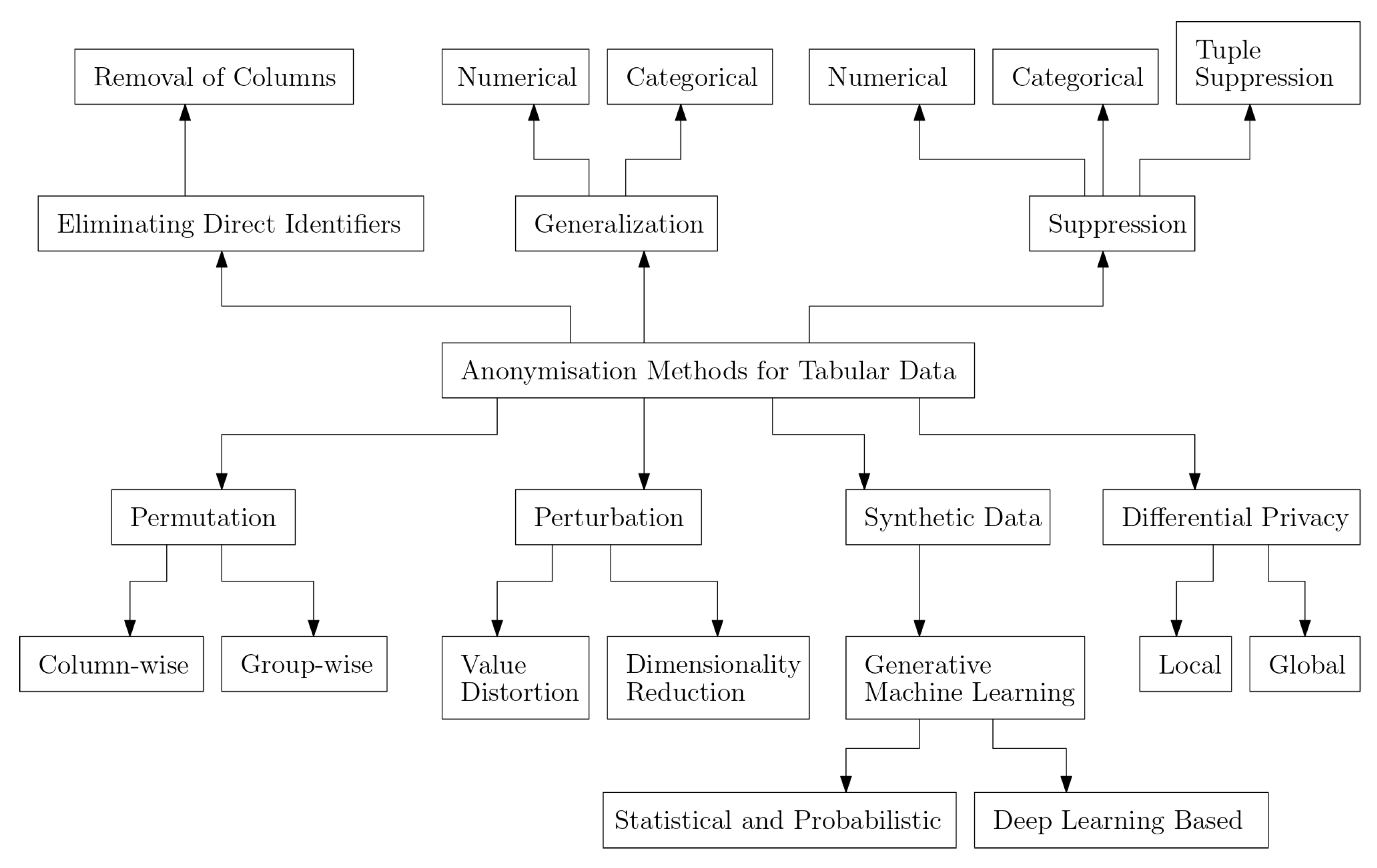
- Terminology and taxonomy establishment of anonymization methods for tabular data:This review introduces a unifying terminology for anonymization methods specific to tabular data. Furthermore, the paper presents a novel taxonomy that categorizes these methods, providing a structured framework that enhances clarity and organization within tabular data anonymization.
- Comprehensive summary of information loss, utility loss, and privacy metrics in the context of anonymizing tabular data:By conducting an extensive exploration, this paper offers a comprehensive overview of methods used to quantitatively assess the impact of anonymization on information and utility in tabular data. By providing an overview of the so-called privacy models, along with precise definitions aligned with the established terminology, the paper reviews and explains the trade-offs between privacy protection and data utility, with special attention to the Curse of Dimensionality. This contribution facilitates a deeper understanding of the complex interplay between anonymization and the quality of tabular data.
- Integration of anonymization of tabular data with legal considerations and risk assessments:Last but not least, this review bridges the gap between technical practices and legal considerations by analyzing how state-of-the-art anonymization methods align with case law and legislation. By elucidating the connection between anonymization techniques and the legal context, the paper provides valuable insights into the regulatory landscape surrounding tabular data anonymization. This integration of technical insights with legal implications is essential for researchers, practitioners, and policymakers alike, contributing to a more holistic approach to data anonymization. The paper conducts a risk assessment for privacy metrics and discusses present issues regarding implementing anonymization procedures for tabular data. Further, it examines possible gaps in the interplay of legislation and research from both technical and legal perspectives. Based on the limited sources of literature and case law, conclusions on the evaluation of the procedures were summarized and were partially drawn using deduction.
2. Background
3. Related Work
4. Technical Perspective
4.1. Eliminating Direct Identifiers
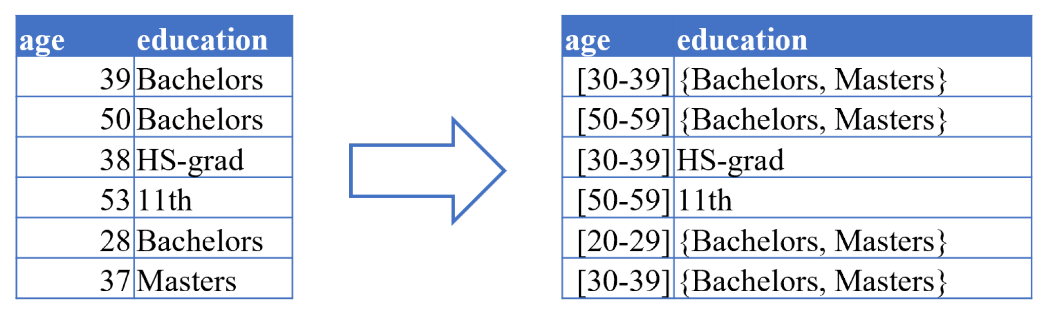
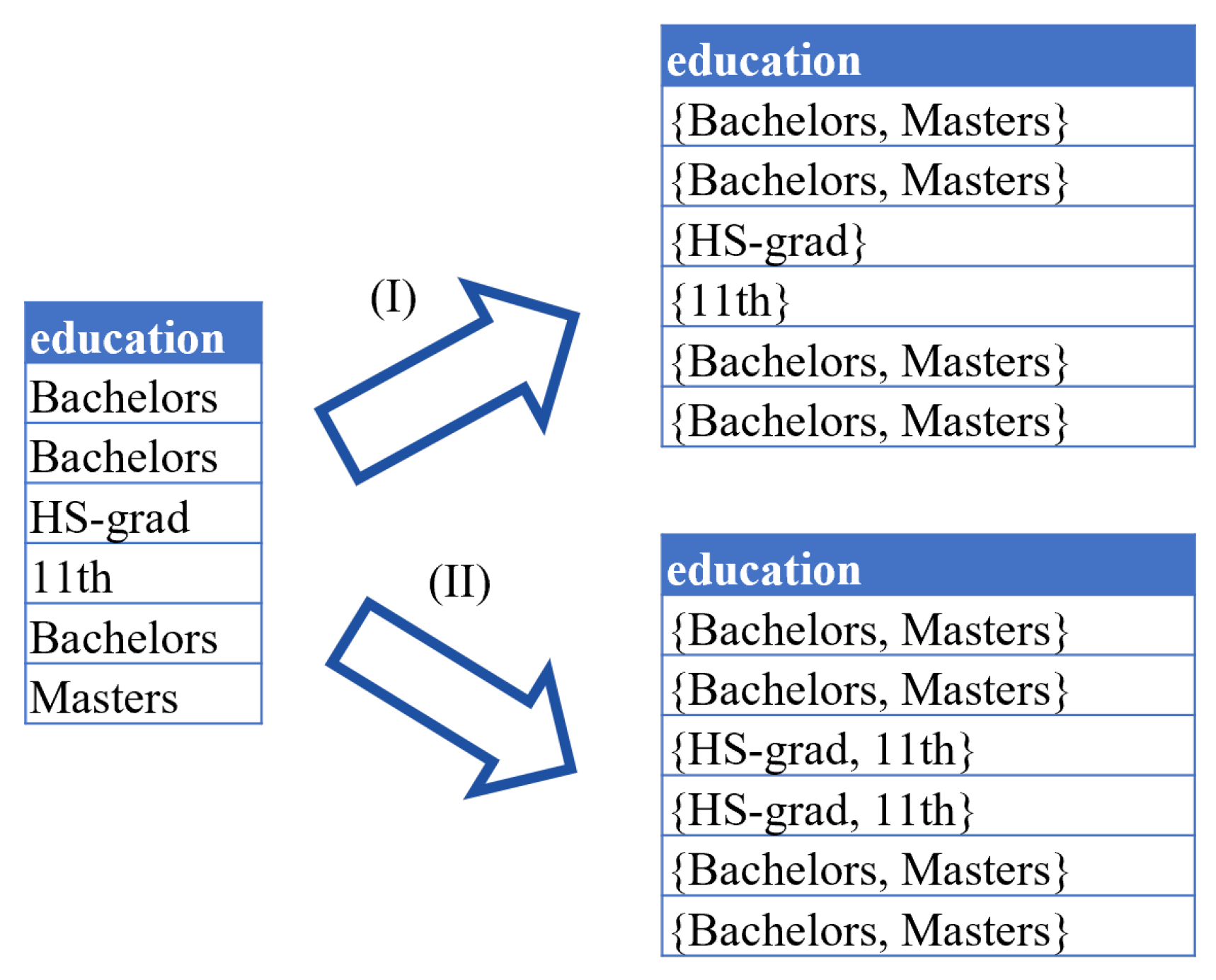
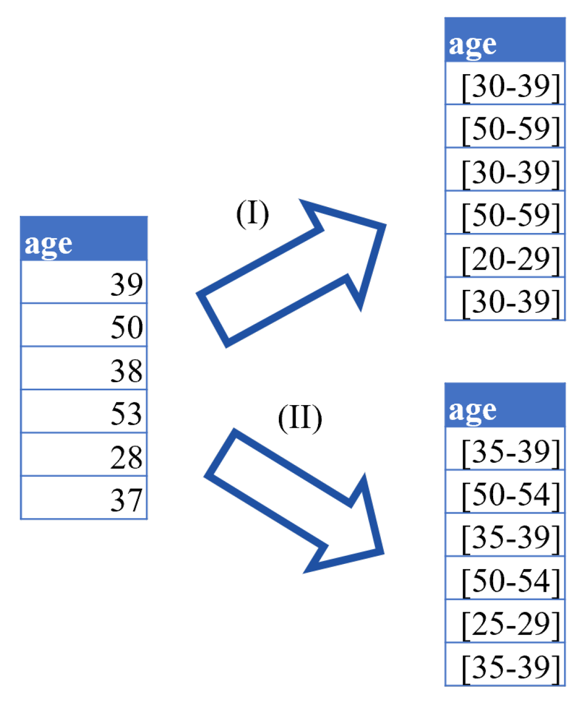
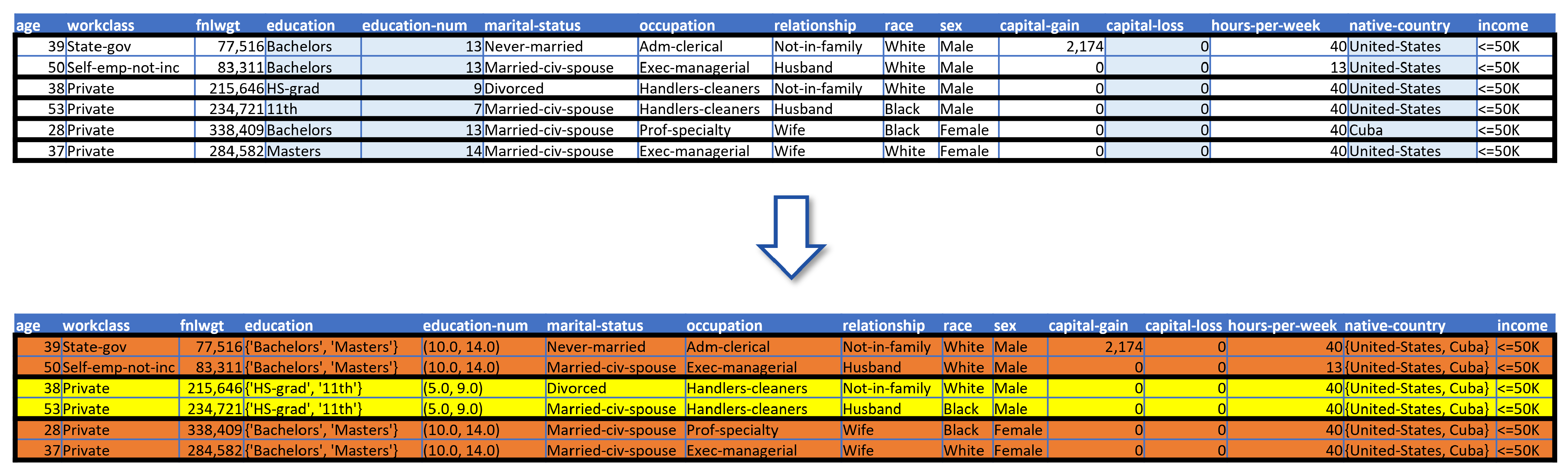
4.2. Generalization
4.3. Suppression
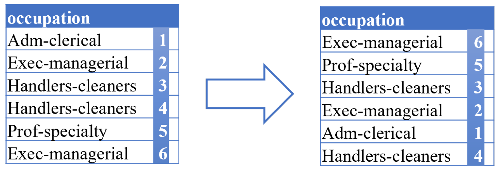
4.4. Permutation
4.5. Perturbation
4.6. Differential Privacy
4.7. Synthetic Data
5. Utility vs. Privacy
5.1. Information Loss
5.2. Utility Loss
5.3. Privacy Models
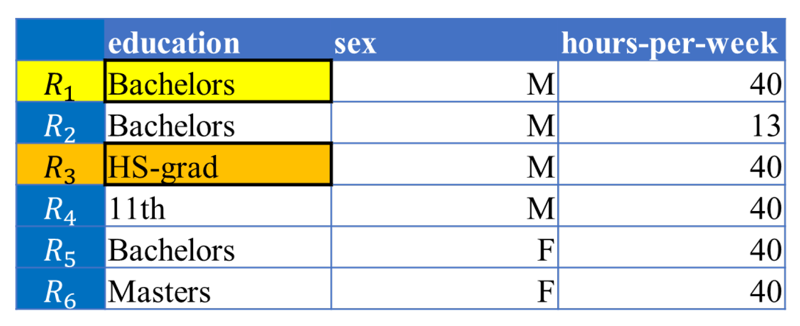
5.3.1. k-Anonymity
5.3.2. l-Diversity
5.3.3. t-Closeness
- D is the dataset;
- P is the relative frequency distribution of all attribute values in the column of the SA in dataset D;
- is the relative frequency distribution of all attribute values in the column of the SA within that is an equivalence class of dataset D and is obtained by a given QI;
- is the EMD between two relative frequency distributions and depends on the attributes’ value type.
- o is the number of distinct integer attribute values in the SA column;
- P and Q are two relative frequency distributions as histograms (integers are ordered in ascending order).
- o is the number of distinct categorical attribute values in the SA column;
- P and Q are two relative frequency distributions as histograms (integers are ordered in ascending order).
5.4. Re-Identification Risk Quantification
- ;
- ;
- ;
- .
5.5. Curse of Dimensionality
6. Legal Perspective
6.1. Synopsis of the Problem
6.2. Recital 26
6.3. Absolute Personal Reference/Zero-Risk Approach
6.4. Relative Personal Reference/Risk-Based Approach
6.5. Tightened Relative Personal Reference of the EU’s Court of Justice
6.6. Evaluation Standards for the Risk Assessment of the Techniques
6.7. Legal Evaluation
6.7.1. Identifiers, Quasi-Identifiers, and Sensitive Attributes
6.7.2. k-Anonymity
6.7.3. l-Diversity
6.7.4. t-Closeness
6.7.5. Differential Privacy
6.7.6. Synthetic Data
6.7.7. Risk Assessment Overview
7. Discussion
8. Conclusions
Author Contributions
Funding
Institutional Review Board Statement
Informed Consent Statement
Data Availability Statement
Conflicts of Interest
Abbreviations
| DP | Differential Privacy |
| DP-SGD | Differentially Private Stochastic Gradient Descent |
| ECJ | European Court of Justice |
| EGC | European General Court |
| EU | European Union |
| FMRMR | Fragmentation Minimum Redundancy Maximum Relevance |
| GAN | Generative Adversarial Network |
| GDPR | General Data Protection Regulation |
| HIPAA | Health Insurance Portability and Accountability Act |
| LDA | Linear Discriminant Analysis |
| LSTM | Long Short-Term Memory |
| MIMIC-III | Medical Information Mart for Intensive Care |
| PCA | Principal Component Analysis |
| PPDP | Privacy-preserving data publishing |
| PPGIS | Public Participation Geographic Information System |
| QI | Quasi-Identifier |
| SA | Sensitive Attribute |
| SVD | Singular Value Decomposition |
References
- Weitzenboeck, E.M.; Lison, P.; Cyndecka, M.; Langford, M. The GDPR and unstructured data: Is anonymization possible? Int. Data Priv. Law 2022, 12, 184–206. [Google Scholar] [CrossRef]
- Samarati, P.; Sweeney, L. Protecting privacy when disclosing information: K-anonymity and its enforcement through generalization and suppression. In Proceedings of the IEEE Symposium on Security and Privacy, Oakland, CA, USA, 3–6 May 1998; pp. 1–19. [Google Scholar]
- Sweeney, L. K-Anonymity: A Model for Protecting Privacy. Int. J. Uncertain. Fuzziness-Knowl.-Based Syst. 2002, 10, 557–570. [Google Scholar] [CrossRef]
- Ford, E.; Tyler, R.; Johnston, N.; Spencer-Hughes, V.; Evans, G.; Elsom, J.; Madzvamuse, A.; Clay, J.; Gilchrist, K.; Rees-Roberts, M. Challenges Encountered and Lessons Learned when Using a Novel Anonymised Linked Dataset of Health and Social Care Records for Public Health Intelligence: The Sussex Integrated Dataset. Information 2023, 14, 106. [Google Scholar] [CrossRef]
- Becker, B.; Kohavi, R. Adult. UCI Machine Learning Repository. 1996. Available online: https://archive-beta.ics.uci.edu/dataset/2/adult (accessed on 15 May 2023).
- Majeed, A.; Lee, S. Anonymization Techniques for Privacy Preserving Data Publishing: A Comprehensive Survey. IEEE Access 2021, 9, 8512–8545. [Google Scholar] [CrossRef]
- Hasanzadeh, K.; Kajosaari, A.; Häggman, D.; Kyttä, M. A context sensitive approach to anonymizing public participation GIS data: From development to the assessment of anonymization effects on data quality. Comput. Environ. Urban Syst. 2020, 83, 101513. [Google Scholar] [CrossRef]
- Olatunji, I.E.; Rauch, J.; Katzensteiner, M.; Khosla, M. A review of anonymization for healthcare data. In Big Data; Mary Ann Liebert, Inc.: New Rochelle, NY, USA, 2022. [Google Scholar]
- Prasser, F.; Kohlmayer, F. Putting statistical disclosure control into practice: The ARX data anonymization tool. In Medical Data Privacy Handbook; Springer: Cham, Switzerland, 2015; pp. 111–148. [Google Scholar]
- Jakob, C.E.M.; Kohlmayer, F.; Meurers, T.; Vehreschild, J.J.; Prasser, F. Design and evaluation of a data anonymization pipeline to promote Open Science on COVID-19. Sci. Data 2020, 7, 435. [Google Scholar] [CrossRef]
- Malin, B.; Loukides, G.; Benitez, K.; Clayton, E.W. Identifiability in biobanks: Models, measures, and mitigation strategies. Hum. Genet. 2011, 130, 383–392. [Google Scholar] [CrossRef]
- Ram Mohan Rao, P.; Murali Krishna, S.; Siva Kumar, A. Privacy preservation techniques in big data analytics: A survey. J. Big Data 2018, 5, 33. [Google Scholar] [CrossRef]
- Haber, A.C.; Sax, U.; Prasser, F.; the NFDI4Health Consortium. Open tools for quantitative anonymization of tabular phenotype data: Literature review. Briefings Bioinform. 2022, 23, bbac440. [Google Scholar] [CrossRef]
- Wagner, I.; Eckhoff, D. Technical Privacy Metrics. ACM Comput. Surv. 2018, 51, 1–38. [Google Scholar] [CrossRef]
- Vokinger, K.; Stekhoven, D.; Krauthammer, M. Lost in Anonymization—A Data Anonymization Reference Classification Merging Legal and Technical Considerations. J. Law Med. Ethics 2020, 48, 228–231. [Google Scholar] [CrossRef] [PubMed]
- Zibuschka, J.; Kurowski, S.; Roßnagel, H.; Schunck, C.H.; Zimmermann, C. Anonymization Is Dead—Long Live Privacy. In Proceedings of the Open Identity Summit 2019, Garmisch-Partenkirchen, Germany, 28–29 March 2019; Roßnagel, H., Wagner, S., Hühnlein, D., Eds.; Gesellschaft für Informatik: Bonn, Germany, 2019; pp. 71–82. [Google Scholar]
- Rights (OCR), Office for Civil. Methods for De-Identification of PHI. HHS.gov. 2012. Available online: https://www.hhs.gov/hipaa/for-professionals/privacy/special-topics/de-identification/index.html (accessed on 21 July 2023).
- Gionis, A.; Tassa, T. k-Anonymization with Minimal Loss of Information. IEEE Trans. Knowl. Data Eng. 2009, 21, 206–219. [Google Scholar] [CrossRef]
- Terrovitis, M.; Mamoulis, N.; Kalnis, P. Local and global recoding methods for anonymizing set-valued data. VLDB J. 2011, 20, 83–106. [Google Scholar] [CrossRef]
- Agrawal, R.; Srikant, R. Privacy-Preserving Data Mining. In Proceedings of the SIGMOD ’00: Proceedings of the 2000 ACM SIGMOD International Conference on Management of Data, Dallas, TX, USA, 16–18 May 2000; Association for Computing Machinery: New York, NY, USA, 2000; pp. 439–450. [Google Scholar] [CrossRef]
- Bayardo, R.; Agrawal, R. Data privacy through optimal k-anonymization. In Proceedings of the 21st International Conference on Data Engineering (ICDE’05), Tokyo, Japan, 5–8 April 2005; pp. 217–228. [Google Scholar] [CrossRef]
- Dwork, C. Differential Privacy. In Automata, Languages and Programming, Proceedings of the 33rd International Colloquium on Automata, Languages and Programming, Part II (ICALP 2006), Venice, Italy, 10–14 July 2006; Springer: Berlin/Heidelberg, Germany, 2006; Volume 4052, pp. 1–12. [Google Scholar]
- Wang, T.; Zhang, X.; Feng, J.; Yang, X. A Comprehensive Survey on Local Differential Privacy toward Data Statistics and Analysis. Sensors 2020, 20, 7030. [Google Scholar] [CrossRef]
- Dwork, C.; Roth, A. The algorithmic foundations of differential privacy. Found. Trends Theor. Comput. Sci. 2014, 9, 211–407. [Google Scholar] [CrossRef]
- Wang, Y.; Wu, X.; Hu, D. Using Randomized Response for Differential Privacy Preserving Data Collection. In Proceedings of the EDBT/ICDT Workshops, Bordeaux, France, 15 March 2016. [Google Scholar]
- Abadi, M.; Chu, A.; Goodfellow, I.; McMahan, H.B.; Mironov, I.; Talwar, K.; Zhang, L. Deep Learning with Differential Privacy. In Proceedings of the 2016 ACM SIGSAC Conference on Computer and Communications Security, Vienna, Austria, 24–28 October 2016; pp. 308–318. [Google Scholar] [CrossRef]
- van der Maaten, L.; Hannun, A.Y. The Trade-Offs of Private Prediction. arXiv 2020, arXiv:2007.05089. [Google Scholar]
- McKenna, R.; Miklau, G.; Sheldon, D. Winning the NIST Contest: A scalable and general approach to differentially private synthetic data. arXiv 2021, arXiv:2108.04978. [Google Scholar] [CrossRef]
- Aggarwal, C.C.; Yu, P.S. A condensation approach to privacy preserving data mining. In Advances in Database Technology-EDBT 2004, Proceedings of the International Conference on Extending Database Technology, Crete, Greece, 14–18 March 2004; Springer: Berlin/Heidelberg, Germany, 2004; pp. 183–199. [Google Scholar]
- Jiang, X.; Ji, Z.; Wang, S.; Mohammed, N.; Cheng, S.; Ohno-Machado, L. Differential-Private Data Publishing Through Component Analysis. Trans. Data Priv. 2013, 6, 19–34. [Google Scholar]
- Xu, S.; Zhang, J.; Han, D.; Wang, J. Singular value decomposition based data distortion strategy for privacy protection. Knowl. Inf. Syst. 2006, 10, 383–397. [Google Scholar] [CrossRef]
- Soria-Comas, J.; Domingo-Ferrer, J. Mitigating the Curse of Dimensionality in Data Anonymization. In Proceedings of the Modeling Decisions for Artificial Intelligence: 16th International Conference, MDAI 2019, Milan, Italy, 4–6 September 2019; Springer: Berlin/Heidelberg, Germany, 2019; pp. 346–355. [Google Scholar]
- Xu, L.; Veeramachaneni, K. Synthesizing Tabular Data using Generative Adversarial Networks. arXiv 2018, arXiv:1811.11264. [Google Scholar]
- Park, N.; Mohammadi, M.; Gorde, K.; Jajodia, S.; Park, H.; Kim, Y. Data Synthesis based on Generative Adversarial Networks. arXiv 2018, arXiv:1806.03384. [Google Scholar] [CrossRef]
- Xu, L.; Skoularidou, M.; Cuesta-Infante, A.; Veeramachaneni, K. Modeling Tabular data using Conditional GAN. arXiv 2019, arXiv:1907.00503. [Google Scholar]
- Xie, L.; Lin, K.; Wang, S.; Wang, F.; Zhou, J. Differentially Private Generative Adversarial Network. arXiv 2018, arXiv:1802.06739. [Google Scholar]
- Kunar, A.; Birke, R.; Zhao, Z.; Chen, L. DTGAN: Differential Private Training for Tabular GANs. arXiv 2021, arXiv:2107.02521. [Google Scholar]
- Zakerzadeh, H.; Aggrawal, C.C.; Barker, K. Towards Breaking the Curse of Dimensionality for High-Dimensional Privacy. In Proceedings of the 2014 SIAM International Conference on Data Mining, Philadelphia, PA, USA, 24–26 April 2014. [Google Scholar]
- Aggarwal, C.C. On K-Anonymity and the Curse of Dimensionality. In Proceedings of the VLDB ’05: 31st International Conference on Very Large Data Bases, Trondheim, Norway, 30 August–2 September 2005; pp. 901–909. [Google Scholar]
- Salas, J.; Torra, V. A General Algorithm for k-anonymity on Dynamic Databases. In Proceedings of the DPM/CBT@ESORICS, Barcelona, Spain, 6–7 September 2018. [Google Scholar]
- Xu, J.; Wang, W.; Pei, J.; Wang, X.; Shi, B.; Fu, A. Utility-based anonymization for privacy preservation with less information loss. SIGKDD Explor. 2006, 8, 21–30. [Google Scholar] [CrossRef]
- LeFevre, K.; DeWitt, D.; Ramakrishnan, R. Mondrian Multidimensional K-Anonymity. In Proceedings of the 22nd International Conference on Data Engineering (ICDE’06), Atlanta, GA, USA, 3–8 April 2006; p. 25. [Google Scholar] [CrossRef]
- Elabd, E.; Abd elkader, H.; Mubarak, A.A. L—Diversity-Based Semantic Anonymaztion for Data Publishing. Int. J. Inf. Technol. Comput. Sci. 2015, 7, 1–7. [Google Scholar] [CrossRef]
- Wang, X.; Chou, J.K.; Chen, W.; Guan, H.; Chen, W.; Lao, T.; Ma, K.L. A Utility-Aware Visual Approach for Anonymizing Multi-Attribute Tabular Data. IEEE Trans. Vis. Comput. Graph. 2018, 24, 351–360. [Google Scholar] [CrossRef]
- Machanavajjhala, A.; Gehrke, J.; Kifer, D.; Venkitasubramaniam, M. L-diversity: Privacy beyond k-anonymity. In Proceedings of the 22nd International Conference on Data Engineering (ICDE’06), Atlanta, GA, USA, 3–8 April 2006; p. 24. [Google Scholar] [CrossRef]
- Li, N.; Li, T.; Venkatasubramanian, S. t-Closeness: Privacy Beyond k-Anonymity and l-Diversity. In Proceedings of the 2007 IEEE 23rd International Conference on Data Engineering, Istanbul, Turkey, 15 April 2006–20 April 2007; pp. 106–115. [Google Scholar] [CrossRef]
- Vatsalan, D.; Rakotoarivelo, T.; Bhaskar, R.; Tyler, P.; Ladjal, D. Privacy risk quantification in education data using Markov model. Br. J. Educ. Technol. 2022, 53, 804–821. [Google Scholar] [CrossRef]
- Díaz, J.S.P.; García, Á.L. Comparison of machine learning models applied on anonymized data with different techniques. arXiv 2023, arXiv:2305.07415. [Google Scholar]
- CSIRO. Metrics and Frameworks for Privacy Risk Assessments, CSIRO: Canberra, Australia, Adopted on 12 July 2021. 2021. Available online: https://www.csiro.au/en/research/technology-space/cyber/Metrics-and-frameworks-for-privacy-risk-assessments (accessed on 4 June 2023).
- Bellman, R. Dynamic Programming, 1st ed.; Princeton University Press: Princeton, NJ, USA, 1957. [Google Scholar]
- Ding, C.; Peng, H. Minimum redundancy feature selection from microarray gene expression data. In Proceedings of the 2003 IEEE Bioinformatics Conference. CSB2003, Stanford, CA, USA, 11–14 August 2003; pp. 523–528. [Google Scholar] [CrossRef]
- Domingo-Ferrer, J.; Soria-Comas, J. Multi-Dimensional Randomized Response. arXiv 2020, arXiv:2010.10881. [Google Scholar]
- Kühling, J.; Buchner, B. (Eds.) Datenschutz-Grundverordnung BDSG: Kommentar, 3rd ed.; C.H.Beck: Bayern, Germany, 2020. [Google Scholar]
- Article 29 Data Protection Working Party. Opinion 4/2007 on the Concept of Personal Data, WP136, Adopted on 20 June 2007. 2007. Available online: https://ec.europa.eu/justice/article-29/documentation/opinion-recommendation/files/2007/wp136en.pdf (accessed on 5 May 2023).
- Auer-Reinsdorff, A.; Conrad, I. (Eds.) Früher unter dem Titel: Beck’sches Mandats-Handbuch IT-Recht. In Handbuch IT-und Datenschutzrecht, 2nd ed.; C.H.Beck: Bayern, Germany, 2016. [Google Scholar]
- Paal, B.P.; Pauly, D.A.; Ernst, S. Datenschutz-Grundverordnung, Bundesdatenschutzgesetz; C.H.Beck: Bayern, Germany, 2021. [Google Scholar]
- Specht, L.; Mantz, R. Handbuch europäisches und deutsches Datenschutzrecht. In Bereichsspezifischer Datenschutz in Privatwirtschaft und öffentlichem Sektor; C.H.Beck: München, Germany, 2019. [Google Scholar]
- Case T-557/20; Single Resolution Board v European Data Protection Supervisor. ECLI:EU:T:2023:219. Official Journal of the European Union: Brussel, Belgium, 2023. Available online: https://eur-lex.europa.eu/legal-content/EN/TXT/PDF/?uri=CELEX:62020TA0557 (accessed on 1 July 2023).
- Groos, D.; van Veen, E.B. Anonymised data and the rule of law. Eur. Data Prot. L. Rev. 2020, 6, 498. [Google Scholar] [CrossRef]
- Finck, M.; Pallas, F. They who must not be identified—distinguishing personal from non-personal data under the GDPR. Int. Data Priv. Law 2020, 10, 11–36. [Google Scholar] [CrossRef]
- Article 29 Data Protection Working Party. Opinion 5/2014 on Anonymisation Techniques; WP216, Adopted on 10 April 2014; Directorate-General for Justice and Consumers: Brussel, Belgium, 2014; Available online: https://ec.europa.eu/justice/article-29/documentation/opinion-recommendation/files/2014/wp216_en.pdf (accessed on 1 July 2023).
- Bergt, M. Die Bestimmbarkeit als Grundproblem des Datenschutzrechts—Überblick über den Theorienstreit und Lösungsvorschlag. Z. Datenschutz 2015, 365, 345–396. [Google Scholar]
- Burkert, C.; Federrath, H.; Marx, M.; Schwarz, M. Positionspapier zur Anonymisierung unter der DSGVO unter Besonderer Berücksichtigung der TK-Branche. Konsultationsverfahren des BfDI. 10 February 2020. Available online: https://www.bfdi.bund.de/SharedDocs/Downloads/DE/Konsultationsverfahren/1_Anonymisierung/Positionspapier-Anonymisierung.html (accessed on 11 May 2023).
- Case C-582/14; Patrick Breyer v Bundesrepublik Deutschland. ECLI:EU:C:2016:779. Court of Justice of the European Union: Brussel, Belgium, 2016. Available online: https://eur-lex.europa.eu/legal-content/EN/TXT/PDF/?uri=CELEX:62014CJ0582 (accessed on 1 July 2023).
- Schwartmann, R.; Jaspers, A.; Lepperhoff, N.; Weiß, S.; Meier, M. Practice Guide to Anonymising Personal Data; Foundation for Data Protection, Leipzig 2022. Available online: https://stiftungdatenschutz.org/fileadmin/Redaktion/Dokumente/Anonymisierung_personenbezogener_Daten/SDS_Practice_Guide_to_Anonymising-Web-EN.pdf (accessed on 10 June 2023).
- Bischoff, C. Pseudonymisierung und Anonymisierung von personenbezogenen Forschungsdaten im Rahmen klinischer Prüfungen von Arzneimitteln (Teil I)-Gesetzliche Anforderungen. Pharma Recht 2020, 6, 309–388. [Google Scholar]
- Simitis, S.; Hornung, G.; Spiecker gen. Döhmann, I. Datenschutzrecht: DSGVO mit BDSG; Nomos: Baden-Baden, Germany, 2019; Volume 1. [Google Scholar]
- Csányi, G.M.; Nagy, D.; Vági, R.; Vadász, J.P.; Orosz, T. Challenges and Open Problems of Legal Document Anonymization. Symmetry 2021, 13, 1490. [Google Scholar] [CrossRef]
- Koll, C.E.; Hopff, S.M.; Meurers, T.; Lee, C.H.; Kohls, M.; Stellbrink, C.; Thibeault, C.; Reinke, L.; Steinbrecher, S.; Schreiber, S.; et al. Statistical biases due to anonymization evaluated in an open clinical dataset from COVID-19 patients. Sci. Data 2022, 9, 776. [Google Scholar] [CrossRef]
- Dewes, A. Verfahren zur Anonymisierung und Pseudonymisierung von Daten. In Datenwirtschaft und Datentechnologie: Wie aus Daten Wert Entsteht; Springer: Berlin/Heidelberg, Germany, 2022; pp. 183–201. [Google Scholar] [CrossRef]
- Giomi, M.; Boenisch, F.; Wehmeyer, C.; Tasnádi, B. A Unified Framework for Quantifying Privacy Risk in Synthetic Data. arXiv 2022, arXiv:2211.10459. [Google Scholar] [CrossRef]
- López, C.A.F. On the legal nature of synthetic data. In Proceedings of the NeurIPS 2022 Workshop on Synthetic Data for Empowering ML Research, New Orleans, LA, USA, 2 December 2022. [Google Scholar]
- Veale, M.; Binns, R.; Edwards, L. Algorithms that Remember: Model Inversion Attacks and Data Protection Law. Philos. Trans. R. Soc. Math. Phys. Eng. Sci. 2018, 376, 20180083. [Google Scholar] [CrossRef]
- Purtova, N. The law of everything. Broad concept of personal data and future of EU data protection law. Law Innov. Technol. 2018, 10, 40–81. [Google Scholar] [CrossRef]


| No. | Direct Identifier | No. | Direct Identifier |
|---|---|---|---|
| 1 | Names | 10 | Social security numbers |
| 2 | All geographic subdivisions smaller than a state | 11 | IP addresses |
| 3 | All elements of dates (except year) directly related to an individual | 12 | Medical record numbers |
| 4 | Telephone numbers | 13 | Biometric identifiers, including finger and voice prints |
| 5 | Vehicle identifiers and serial numbers | 14 | Health plan beneficiary numbers |
| 6 | Fax numbers | 15 | Full-face photographs and any comparable images |
| 7 | Device identifiers and serial numbers | 16 | Account numbers |
| 8 | Email addresses | 17 | Any other unique identifier |
| 9 | URLs | 18 | Certificate/license numbers |
| Measurement | Method |
|---|---|
| Information loss | Conditional entropy [18] |
| Monotone entropy [18] | |
| Non-uniform entropy [18] | |
| Information loss on a per-attribute basis [38] | |
| Relative condensation loss [39] | |
| Euclidean distance [40] | |
| Utility loss | Average group size [41] |
| Normalized average equivalence class size metric [42] | |
| Discernibility metric [21,42,43] | |
| Proportion of suppressed records | |
| ML utility | |
| Earth Mover Distance [44] | |
| z-Test statistics [7] | |
| Privacy models | k-Anonymity [3] |
| Mondrian multi-dimensional k-anonymity [42] | |
| l-Diversity [45] | |
| t-Closeness [46] | |
| Privacy probability of non-re-identification [47] |
| Singling Out | Linkability | Inference | |
|---|---|---|---|
| k-Anonymity | + | ||
| l-Diversity | |||
| t-Closeness | |||
| DP | + | ||
| Synthetic data | + | + |
Disclaimer/Publisher’s Note: The statements, opinions and data contained in all publications are solely those of the individual author(s) and contributor(s) and not of MDPI and/or the editor(s). MDPI and/or the editor(s) disclaim responsibility for any injury to people or property resulting from any ideas, methods, instructions or products referred to in the content. |
© 2023 by the authors. Licensee MDPI, Basel, Switzerland. This article is an open access article distributed under the terms and conditions of the Creative Commons Attribution (CC BY) license (https://creativecommons.org/licenses/by/4.0/).
Share and Cite
Aufschläger, R.; Folz, J.; März, E.; Guggumos, J.; Heigl, M.; Buchner, B.; Schramm, M. Anonymization Procedures for Tabular Data: An Explanatory Technical and Legal Synthesis. Information 2023, 14, 487. https://doi.org/10.3390/info14090487
Aufschläger R, Folz J, März E, Guggumos J, Heigl M, Buchner B, Schramm M. Anonymization Procedures for Tabular Data: An Explanatory Technical and Legal Synthesis. Information. 2023; 14(9):487. https://doi.org/10.3390/info14090487
Chicago/Turabian StyleAufschläger, Robert, Jakob Folz, Elena März, Johann Guggumos, Michael Heigl, Benedikt Buchner, and Martin Schramm. 2023. "Anonymization Procedures for Tabular Data: An Explanatory Technical and Legal Synthesis" Information 14, no. 9: 487. https://doi.org/10.3390/info14090487