Multiple Explainable Approaches to Predict the Risk of Stroke Using Artificial Intelligence

Abstract

Stroke occurs when a brain’s blood artery ruptures or the brain’s blood supply is interrupted. Due to rupture or obstruction, the brain’s tissues cannot receive enough blood and oxygen. Stroke is a common cause of mortality among older people. Hence, loss of life and severe brain damage can be avoided if stroke is recognized and diagnosed early. Healthcare professionals can discover solutions more quickly and accurately using artificial intelligence (AI) and machine learning (ML). As a result, we have shown how to predict stroke in patients using heterogeneous classifiers and explainable artificial intelligence (XAI). The multistack of ML models surpassed all other classifiers, with accuracy, recall, and precision of 96%, 96%, and 96%, respectively. Explainable artificial intelligence is a collection of frameworks and tools that aid in understanding and interpreting predictions provided by machine learning algorithms. Five diverse XAI methods, such as Shapley Additive Values (SHAP), ELI5, QLattice, Local Interpretable Model-agnostic Explanations (LIME) and Anchor, have been used to decipher the model predictions. This research aims to enable healthcare professionals to provide patients with more personalized and efficient care, while also providing a screening architecture with automated tools that can be used to revolutionize stroke prevention and treatment.

1. Introduction

A blockage or leak in the blood vessels causes the brain’s blood flow to be stopped or diminished, which results in a stroke. When this happens, the brain’s cells start to degrade as a result of lack of nutrition and oxygen [1]. Stroke is a cerebrovascular condition. This suggests that it has an effect on the blood vessels that supply the brain with oxygen. If the brain is not given adequate oxygen, damage may start to occur [2]. Medical help is needed immediately. Some strokes can be deadly or leave a person incapacitated, despite the fact that many of them are treatable [3,4,5,6].

Stroke symptoms appear unexpectedly, and they might differ from person to person. Signs of a stroke include dizziness, problems speaking or understanding, blurred or lost vision in one or both eyes, a lack of sensation of the arms, legs, or face, usually on a single side of the body or issues with coordination or balance, walking or mobility issues, fainting or seizures and extreme headaches that have no apparent reason. Other stroke symptoms that are less typical may include sudden nausea, momentary loss of consciousness, fainting, confusion, seizures, or coma [7,8,9,10]. The treatment process for stroke is depicted in Figure 1.

Prediction of stroke can be made by using AI/ML classifiers. One such field where machine learning (ML) could have a big impact on society is the healthcare sector. In a market of smart watches, fit bits, and other devices that continuously capture a wealth of health data, the use of machine learning to assess health data is becoming widespread. Machine learning may prove to be the solution to the healthcare sector’s rising costs as well as to strengthening the relationship between patients and doctors. Machine learning and big data solutions can be used for a variety of health-related applications such as diagnosis, prognosis, decision support systems, helping doctors optimise prescriptions and treatments, helping patients decide when and whether to schedule follow-up appointments and many more [11,12].

Artificial intelligence (AI) algorithms carry out sophisticated operations on very large amounts of data. These operations include text recognition and imaging, remote health treatment, accurate disease prediction and detection [13]. Explainable AI (XAI) was developed as a result of the realisation that the classifiers must be used in an appropriate manner in order to ensure transparency, accountability, and ethics [14]. The explainability factor gives black-box models new potential and provides healthcare stakeholders the confidence to interpret Machine Learning (ML) and Deep Learning (DL) models. In the healthcare industry, transparency in predictive analysis is essential and XAI is centred on enhancing it [15].

This research focuses on the usage of XAI techniques such as Eli5, SHAP, QLattice, LIME and Anchor for better understanding of stroke predictions [16]. Explainable AI (XAI) is a new area of machine learning that tries to solve how AI systems make decisions in a “black box.” This field examines the steps and models involved in decision making by making it more interpretable and understandable.

Several studies have already employed machine learning algorithms to predict stroke. The contributions of some research studies are described below:

Govindarajan et al. [17] collected data from 507 patients to categorise stroke disease combining machine learning and text mining algorithms. For their analysis, several machine learning algorithms were employed, and the stochastic gradient algorithm (SGD) provided the classification accuracy of 95%. Tazin et al. [18] employed a dataset containing 5110 records, where 249 patients were at risk of having a stroke and 4861 were not. For early stroke prediction, ML algorithms, such as logistic regression (LR), decision tree (DT), random forest (RF), and voting classifier, were utilised. Among these, the RF model outperformed the others with 96% accuracy. Emon et al. [19] proposed a framework for the early prediction of stroke using various machine learning classifiers such as LR, SGD, DT, AdaBoost, Gradient Boosting Classifier (GBC), XGBoost (XGB), and multilayer perceptron (MLP) and compared them with the proposed weighted voting classifier. According to the performance test, weighted voting classifier delivered the highest accuracy of 97%. Sailasya et al. [20] examined a stroke dataset and performed data preprocessing such as label encoding, handling of missing values, and imbalanced data handling. On this dataset, six machine learning techniques were employed. The Naive Bayes algorithm obtained an accuracy of 82% Shoily et al. [21] proposed a new prediction model with several feature selection combinations. They built their model with Naive Bayes, J48, KNN, and RF classifiers. From the above studies, it is evident that ML and AI algorithms have already been utilised to predict stroke risk. This article makes the following contributions to the existing literature:

• The most crucial attributes have been decided upon using four feature selection techniques: Pearson’s correlation, Mutual information, Particle swarm optimization and Harris Hawks algorithm. Comparison of the feature selection methods have been made in this study.
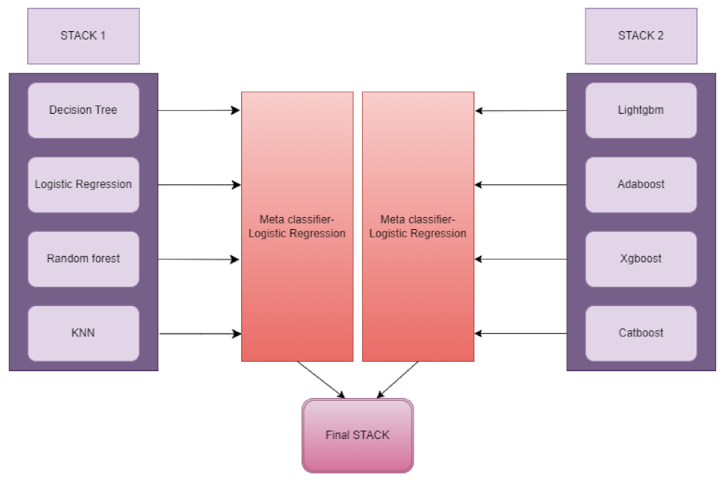
• A novel customised “ensemble-stacking” architecture was designed and used to improve the performance utilizing baseline classifiers.
• This is a unique study that used five XAI techniques, such as LIME, SHAP, ELI5, Anchor and Qlattice, on the dataset to demystify stroke predictions.

The rest of the article is structured as follows: Section 2 comprises materials and methods. The results are extensively described in Section 3. Section 4 comprises the conclusion and future scope.

2. Materials and Methods

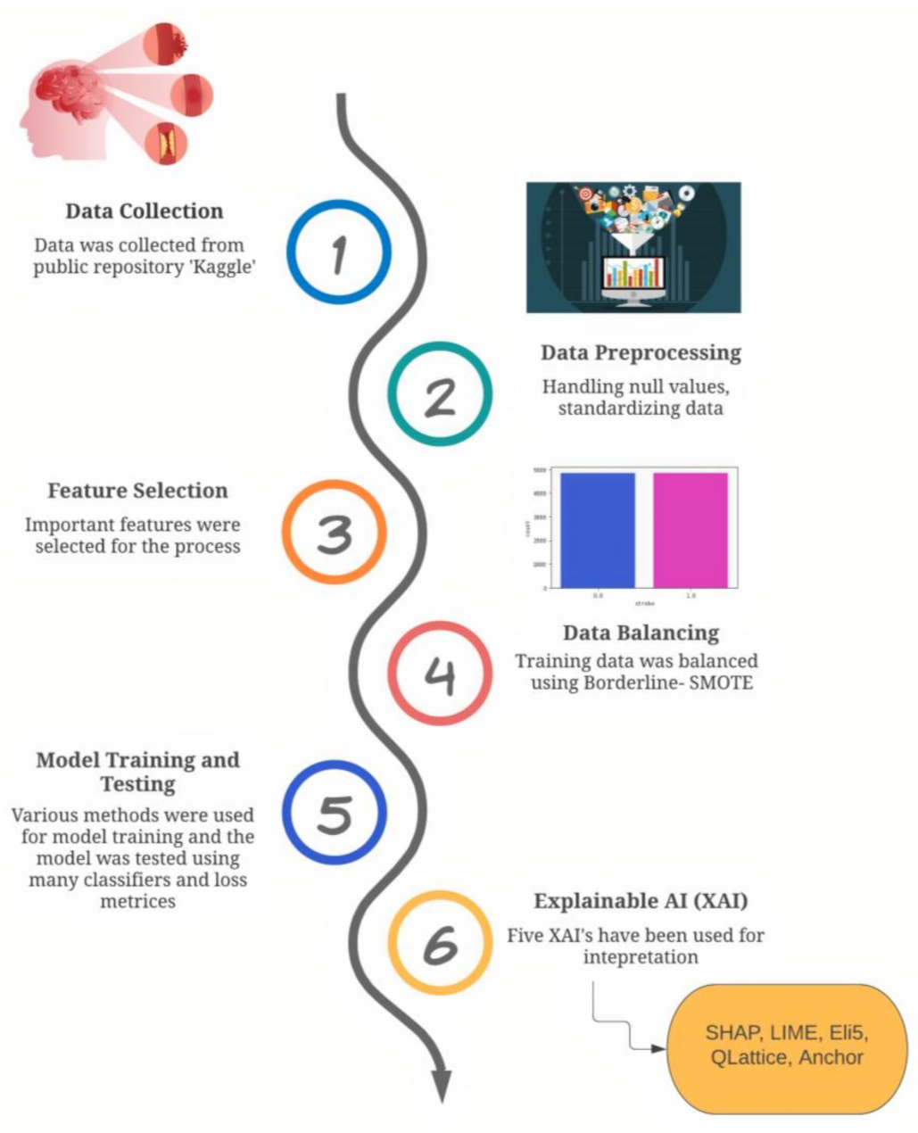
2.1. Data Description

In this research, we made use of a publicly available stroke dataset [22]. This dataset has information on 5110 patients with 12 attributes. This dataset has stroke as the target variable (binary classification problem). Out of 5110 patients, 4869 did not have stroke and 249 had stroke. The attribute “BMI” had 201 null values. Since the median is unaffected by outliers, it was used to impute the missing values for continuous variables. The dataset’s attributes are described in

Table 1. An overview of our dataset’s attributes.

Attribute Number	Attribute Name Mentioned in the Data File	Attribute Name	Description of the Attribute
1	id	Id	Unique identifier number for each patient
2	gender	Gender	Female, Male, Other
3	age	Age (years)	Patient’s age
4	hypertension	Hypertension (0/1)	If patient has hypertension (1) or no hypertension (0)
5	heart_disease	Heart disease (0/1)	If patient has any heart disease (1) or no heart disease (0)
6	ever_married	Yes-married No-not married	Patient’s marital status
7	work_type	Work type	If the patient is a child or has a government job, if they have never worked, if they work in a private organization, or if they are self-employed
8	Residence_type	Residence type	If the patient lives in urban residential area or rural residential area
9	avg_glucose_level	Average glucose level	Average glucose level present in the blood
10	bmi	BMI	Body mass index of the patient
11	smoking_status	Smoking status	If the patient formerly smoked, if they have never smoked, if they smoke or Unknown (information is unavailable)
12	stroke	0-no stroke 1-had stroke	If the patient had stroke (1) or did not have stoke (0)

.

2.2. Data Preprocessing

Raw data are transformed into usable and understandable forms through data preprocessing. There are several challenges associated with raw datasets, including flaws as well as inconsistent behaviour, lack of trends, and inconsistency. It is also necessary to perform preprocessing in order to handle missing values and inconsistencies [23]. Preprocessing of the dataset was performed, and it needed a few additional procedures to be prepared for deployment. The missing values in the ‘bmi’ attribute were replaced by its median. Since the attribute’s ‘id’, ‘ever_married’, and ‘work_type’ had little statistical relevance, we eliminated them.

The violin plot for attributes such as age and average_glucose_level is shown in Figure 2. (a) Patients with strokes ranged in age from roughly 40 to 80 years old, while those without strokes ranged in age from 0 to 80. (b) The majority of patients’ average blood glucose levels ranged from 50 to 130, while the rest ranged from 130 to 300, and these patients did not experience a stroke. Majority of stroke patients had average blood sugar levels between 60 and 130, only a small percentage had levels between 170–300.

The attributes’ variations in relation to the target variable stroke are depicted in Figure 3. While 183 individuals had no hypertension but suffered a stroke, 4429 patients had neither.

Sixty-six patients had both hypertension and stroke, while 432 patients had hypertension but no stroke. A total of 202 patients had a stroke but no heart disease, while 4632 patients had neither. Forty-seven patients had both heart disease and a stroke, while 229 patients had heart disease and no stroke. There were 141 female patients who had a stroke and 2853 female patients who did not. A total of 108 males experienced strokes, compared to 2007 males who were stroke-free. While the smoking status of 1497 patients was unknown and they did not experience a stroke, 47 patients with this same status experienced a stroke. While 70 individuals who formerly smoked suffered strokes, 815 other patients who formerly smoked did not have stroke. Ninety people who had never smoked experienced strokes, while 1802 patients who had never smoked did not. Forty-two smokers who had strokes in comparison to 747 smokers who did not have stroke.

Rescaling the attributes to have a mean of 0 and a variance of 1 is the process of data standardization. Standardization’s objective is to reduce all features to a comparable scale without distorting the variations in the values ranges. For feature scaling, we implemented the standard scaler algorithm. After standardization, outliers have no effect on the data and standardization has no bounding range.

Balancing the dataset facilitates model training by avoiding it from becoming biased towards one class. Data balancing can be performed in two ways: undersampling or oversampling. Despite the fact that undersampling is simple to perform and can improve model run-time, it has certain drawbacks. Eliminating samples from the original dataset can result in the loss of important information. If there are insufficient data, it may also lead to overfitting. Hence, oversampling was proposed in this study. To reduce the possibility of inappropriate model training, we used the Borderline-Synthetic Minority Oversampling Technique (SMOTE) to balance the training dataset data. Oversampling in this approach generates deceptive points from the minority class [24,25]. A comparison of the borderline-SMOTE algorithm’s performance before and after is shown in Figure 4. The testing dataset was not balanced to preserve integrity.

2.3. Feature Selection

Pearson’s Correlation, Mutual information, Particle swarm optimization and Harris Hawks algorithm were utilized in this study to choose the best features. These algorithms assisted in extracting the important attributes and reduced the amount of data.

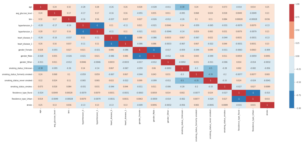
2.3.1. Pearson’s Correlation

Following a preliminary review of the data, the influence of each feature on the result was examined using Pearson’s correlation coefficient analysis. A perfect relationship between the correlation coefficient value “r” and the output is shown if the value was near “−1/1,” whereas a value of 0 denoted there was no correlation. Values of the correlation coefficient that are positive show that the factor had an effect on the result favourably. If it was negative, the effect on the result was the opposite. The basis for the correlation coefficient evaluation approach is the notion that assessing the strength of the link between the characteristics of variables can help evaluate the importance of a feature collection in a dataset [26,27]. Some variables exhibited a positive association, whereas others exhibited a negative correlation. The correlation heatmap is shown in Figure 5.

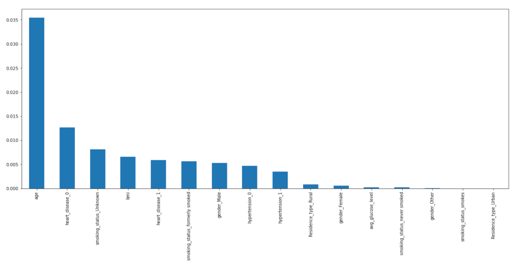
2.3.2. Mutual Information (MI)

A popular feature selection approach is the Mutual Information algorithm [28]. The statistical properties of the dataset are considered by this filtering technique. Entropy, which measures the degree of uncertainty in the features, serves as the foundation for mutual information. The attributes were ranked based on how much each attribute contributes to the target variable, as seen in Figure 6.

2.3.3. Particle Swarm Optimization

An effective global search method is required to solve feature selection issues more effectively. Global search capabilities of evolutionary computation (EC) approaches are well recognized. The EC method known as particle swarm optimization (PSO), which is based on swarm intelligence, is relatively new. PSO is computationally less costly and has a faster convergence rate when compared to other EC algorithms like genetic programming (GP) and genetic algorithms (GAs) [29,30,31,32,33]. Eleven features were selected with this feature selection out of 16 parameters. These selected features are presented in

Table 2. Important features.

Methods Used	Features
Mutual Information	‘age’, ‘heart_disease_0’, ‘smoking_status_Unknown’, ‘bmi’, ‘heart_disease_1’, ‘smoking_status_formerly smoked’, ‘gender_Male’, ‘hypertension_0’, ‘hypertension_1’, ‘Residence_type_Rural’.
Pearson’s Correlation	‘age’, ‘heart_disease_1’, ‘heart_disease_0’, ‘avg_glucose_level’, ‘hypertension_1’, ‘hypertension_0’, ‘smoking_status_formerly smoked’, ‘smoking_status_Unknown’, ‘bmi’, ‘Residence_type_Rural’.
Particle swarm optimization	‘age’, ‘heart_disease_0’, ‘heart_disease_1’, ‘hypertension_0’, ‘hypertension_1’, ‘gender_Male’, ‘gender_Female’, ‘gender_Other’, ‘bmi’, ‘Residence_type_Rural’, ‘Residence_type_Urban’.
Harris Hawks algorithm	‘age’, ‘heart_disease_0’, ‘heart_disease_1’, ‘gender_Male’, ‘gender_Female’, ‘gender_Other’, ‘bmi’, ‘smoking_status_Unknown’, ‘smoking_status_formerly smoked’, ‘smoking_status_never smoked’, ‘smoking_status_smokes’.

.

2.3.4. Harris Hawks Algorithm

Heidari et al. created the Harris Hawks Optimizer (HHO), a swarm-based optimization technique. The basic goal of HHO is to imitate the natural hunting behaviour of the Hawk team and the prey’s flight in order to find solutions to the single-objective problem. In Harris Hawks Optimizer, the best location is represented by the prey, while the hawks’ chasing behaviour reflects the search agent [34,35,36,37,38]. Harris Hawks Optimizer can be used to solve a variety of real-world optimization problems, including those involving discrete and continuous spaces, and can improve the quality of solutions, offer high accuracy in obtaining the best possible parameters, and improve prediction performance [39,40,41,42,43].

2.3.5. Important Features

Important features according to Mutual information, Pearson’s correlation, Particle swarm optimization and Harris Hawks algorithm are listed in Table 2. Age, BMI, hypertension, and heart disease are some characteristics that are consistent. These features were chosen for further analysis.

2.4. Machine Learning Terminologies

The various stages of the machine learning process are data preparation and selection, model selection, model training on the data, performance evaluation, and model deployment. Iterative experimentation and model improvement are frequently used in the process to boost the model’s performance. The development of a model that accurately generalizes to new data and resolves the issue at hand is the ultimate goal of the machine learning process.

Successful hyperparameter tuning is a prerequisite for selecting the best model. The goal of hyperparameter selection is to draw attention to the successful results from earlier training cycles. Adjusting the algorithm’s parameters allow model improvement [27]. In this study, we achieved optimised parameter values using the grid search optimisation technique. Grid search is a tuning method that performs thorough parameter searching by manually examining each value within the specifically defined hyperparameter space.

There are numerous techniques to use machine learning ensemble models, including boosting, stacking, and bagging. By using stacking, we can train several models to address similar problems and then combine the findings to produce a more potent model [44]. Utilising this idea, we constructed three stacks on two different levels. A visual example of stacking is shown in Figure 7. The first stack consisted of logistic regression, decision tree, random forest and K Nearest Neighbours (KNN). The second stack comprised of tree-based algorithms, such as lightgbm, adaboost, catboost and xgboost. Finally, the above stacks were further ensembled to form the final stack.

The results obtained by the models were interpreted using XAI techniques. The XAI models used in this study are:

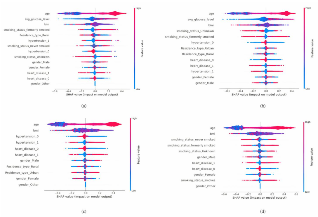
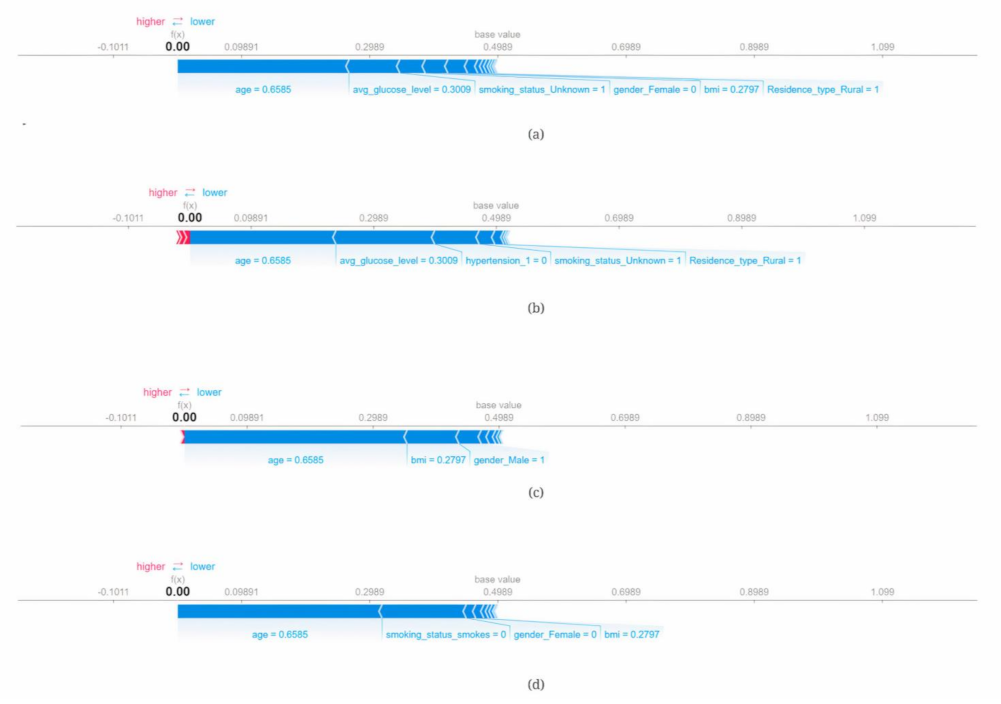
• SHAP (SHapley Additive exPlanations): It uses a model-neutral approach for analysing the output of any machine learning model by figuring out how much each feature contributed to the final prediction.
• LIME (Local Interpretable Model-agnostic Explanations): It is a technique for generating local interpretations of black-box models by approximating them with interpretable models trained on subsets of the data.
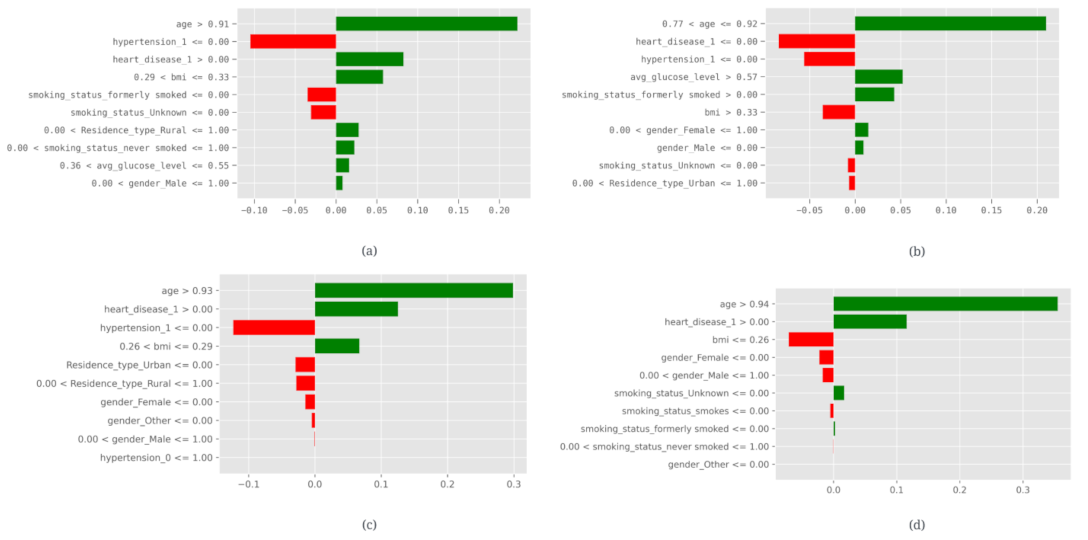
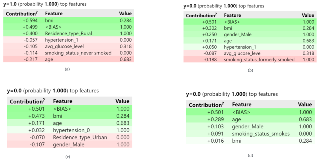
• ELI5 (Explain Like I’m 5): It is a Python library that provides simple explanations of machine learning models using a variety of techniques, including feature importance, decision trees, and permutation feature importance.
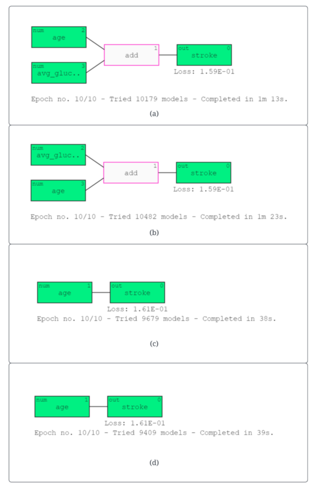
• Qlattice: It is a visualization tool for exploring machine learning models that allows users to interactively explore the model’s decision-making process by visualizing the feature contributions to the final prediction.
• Anchor: It is uses rules and conditions to explain the model output. It uses the evaluation metrics precision and coverage to identify the importance of that particular condition.

A machine learning pipeline is a series of interconnected data processing modules that automate the end-to-end workflow of a machine learning project. It usually entails data preparation, feature engineering, model selection, tuning of the hyperparameters, and evaluation. The pipeline is designed to optimize the performance of the machine learning models by providing a systematic and automated approach to the entire process. Figure 8 shows the ML pipeline used for the study.

3. Results

3.1. Performance Metrics

Using classification metrics such as precision, F-1 score, accuracy, recall and AUC score (Area Under the curve), we have assessed and compared our AI models. Our classifiers try to determine whether a specific patient has a stroke or not.

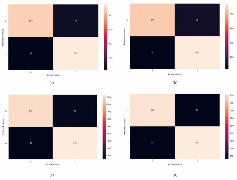
• Accuracy: The accuracy is its capacity to distinguish between patients experiencing a stroke and those who do not correctly. The proportion of true positive and true negative outcomes in all analysed cases should be determined in order to determine the prediction’s accuracy. The mathematical formula is:

  $$Accuracy=\frac{TP+TN}{TP+TN+FN+FP}$$

  (1)
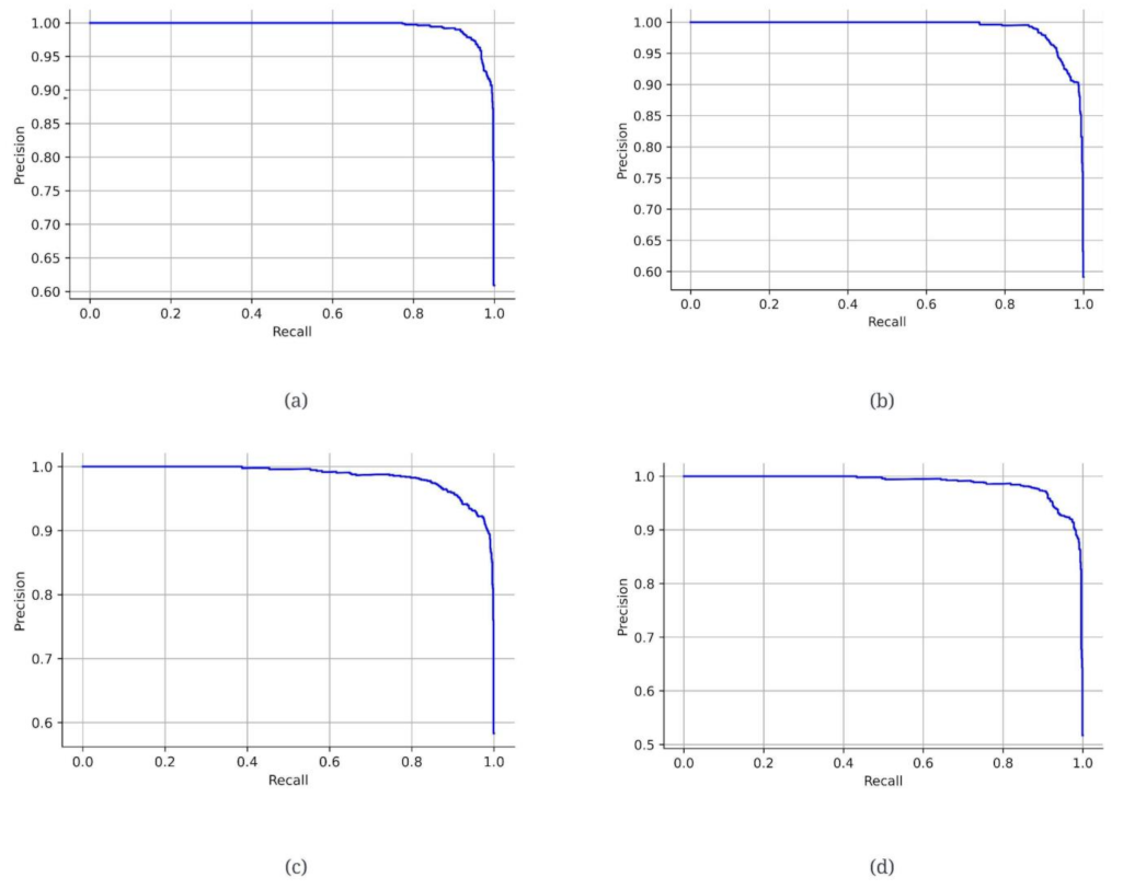
• Precision: It is a statistic that determines the proportion of patients who actually suffered a stroke compared to all other patients. This implies that it also considers patients who have received a false-positive stroke diagnosis. The equation is as follows:

  $$Precision=\frac{TP}{TP+FP}$$

  (2)
• Recall: It is a measure of performance that is described as the ratio of patients who had a stroke accurately to all the patients who had been affected. This statistic puts a focus on false-negative situations. When there are few false-negative cases, the recall is extraordinarily high. It is calculated using the following formula:

  $$Recall=\frac{TP}{TP+FN}$$

  (3)
• F1 score: A evaluation metric that combines a model’s precision and recall scores. It is calculated using the following formula:

  $$F1 score=2\times \frac{precision\times recall}{precision+recall}$$

  (4)
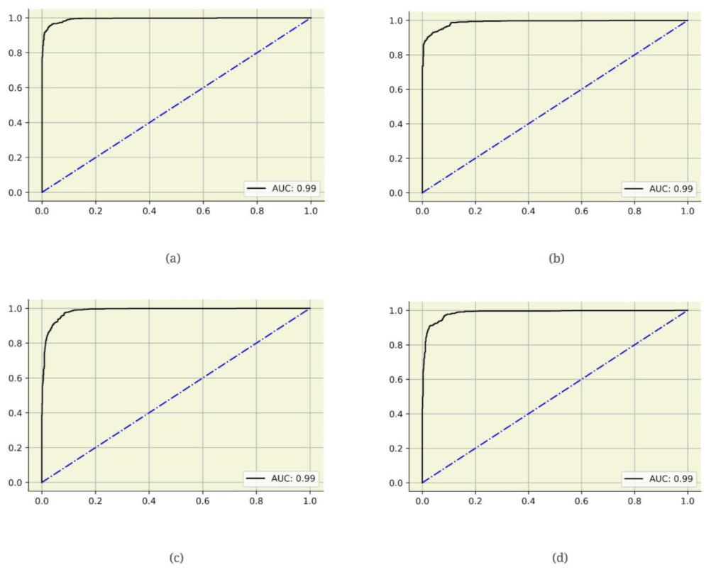
• AUC: The true positive rate versus the false-positive rate for various test scenarios is plotted on the receiver operating characteristic (ROC) curve. It shows how effectively the models distinguish between the binary classifications. The AUC is the region beneath this curve. AUC values that are high show that the classifier is working effectively.

3.2. Model Evaluation

The ML algorithms can precisely estimate a person’s risk of stroke and offer personalised recommendations for prevention and therapy by identifying trends and risk factors. Additionally, they can help medical professionals diagnose patients more quickly and accurately, improving patient outcomes. Using the Python integrated Conda virtual environment, the classifiers were run. Important libraries including pandas, Scikit, seaborn, matplotlib and NumPy were installed. An “Intel^® core (TM) i5” CPU was utilised to train the models, which used 8 GB of RAM. For this study, a 64-bit Windows operating system was taken into consideration.

An 80:20 training-to-testing ratio was used to train all the models. The results from several ML models are summarised in

Table 3. The summary of the findings from the various machine learning models applied in this study with respect to Pearson’s Correlation, Mutual Information, Particle swarm optimization and Harris Hawks algorithm.

Pearson’s Correlation
Model	Accuracy	Precision	Recall	F1-Score	AUC	Log Loss	Hamming Loss	Jaccord Score	MCC
Random Forest	0.92	0.90	0.95	0.93	0.98	2.628	0.076	0.863	0.849
Logistic Regression	0.83	0.80	0.88	0.84	0.90	5.753	0.166	0.728	0.669
Decision Tree	0.89	0.89	0.90	0.89	0.93	3.746	0.108	0.806	0.783
KNN	0.92	0.89	0.95	0.92	0.92	2.752	0.079	0.857	0.842
SVM- Linear kernal	0.83	0.80	0.90	0.84	0.90	5.789	0.167	0.729	0.670
SVM- Sigmoidal kernal	0.59	0.59	0.59	0.59	0.71	14.170	0.410	0.420	0.179
Stack 1	0.92	0.90	0.96	0.92	0.98	2.716	0.078	0.859	0.844
AdaBoost	0.90	0.89	0.92	0.90	0.97	3.445	0.099	0.822	0.800
CatBoost	0.85	0.81	0.92	0.86	0.93	5.274	0.152	0.751	0.700
LGBM	0.95	0.96	0.94	0.95	0.99	1.775	0.051	0.901	0.897
XGB	0.95	0.95	0.95	0.95	0.99	1.846	0.053	0.899	0.893
Stack 2	0.95	0.95	0.95	0.95	0.99	1.722	0.049	0.905	0.900
Final Stack	0.94	0.91	0.96	0.94	0.99	2.219	0.064	0.883	0.872
Mutual information
Model	Accuracy	Precision	Recall	F1-Score	AUC	Log Loss	Hamming Loss	Jaccord score	MCC
Random Forest	0.94	0.92	0.96	0.94	0.98	2.130	0.061	0.887	0.877
Logistic Regression	0.83	0.80	0.89	0.84	0.89	5.735	0.166	0.729	0.671
Decision Tree	0.88	0.88	0.89	0.89	0.92	3.995	0.115	0.795	0.768
KNN	0.94	0.91	0.97	0.94	0.94	2.095	0.060	0.890	0.880
SVM- Linear kernal	0.83	0.80	0.89	0.84	0.89	5.948	0.172	0.721	0.659
SVM- Sigmoidal kernal	0.59	0.60	0.56	0.58	0.67	14.259	0.412	0.407	0.174
Stack 1	0.94	0.91	0.97	0.94	0.99	2.077	0.060	0.890	0.881
AdaBoost	0.90	0.89	0.92	0.90	0.97	3.374	0.097	0.825	0.804
CatBoost	0.84	0.80	0.91	0.85	0.93	5.522	0.159	0.740	0.685
LGBM	0.96	0.96	0.95	0.96	0.99	1.527	0.044	0.915	0.911
XGB	0.95	0.95	0.95	0.95	0.99	1.687	0.048	0.907	0.902
Stack 2	0.96	0.96	0.96	0.96	0.99	1.402	0.040	0.922	0.918
Final Stack	0.95	0.93	0.97	0.95	0.99	1.740	0.050	0.906	0.900
Random Forest	0.94	0.92	0.97	0.94	0.98	2.059	0.059	0.890	0.881
Logistic Regression	0.83	0.81	0.87	0.84	0.91	5.771	0.167	0.725	0.667
Decision Tree	0.91	0.91	0.91	0.91	0.95	3.125	0.090	0.834	0.819
KNN	0.92	0.88	0.97	0.92	0.95	2.823	0.081	0.856	0.840
SVM- Linear kernal	0.83	0.81	0.87	0.84	0.91	5.913	0.171	0.718	0.659
SVM- Sigmoidal kernal	0.56	0.57	0.56	0.56	0.7	15.147	0.438	0.391	0.122
Stack 1	0.94	0.93	0.95	0.94	0.98	2.166	0.062	0.884	0.874
AdaBoost	0.90	0.88	0.94	0.91	0.97	3.338	0.096	0.830	0.808
CatBoost	0.87	0.83	0.94	0.88	0.94	4.510	0.130	0.783	0.745
LGBM	0.95	0.95	0.95	0.95	0.99	1.811	0.052	0.900	0.895
XGB	0.95	0.94	0.96	0.95	0.99	1.740	0.050	0.905	0.899
Stack 2	0.95	0.95	0.95	0.95	0.99	1.775	0.051	0.903	0.897
Final Stack	0.94	0.93	0.95	0.94	0.99	2.059	0.059	0.889	0.880
Particle swarm optimization
Model	Accuracy	Precision	Recall	F1-Score	AUC	Log Loss	Hamming Loss	Jaccord score	MCC
Random Forest	0.93	0.91	0.95	0.93	0.98	2.539	0.073	0.866	0.853
Logistic Regression	0.83	0.80	0.88	0.84	0.89	5.806	0.168	0.725	0.666
Decision Tree	0.91	0.92	0.90	0.91	0.94	3.107	0.089	0.834	0.820
KNN	0.91	0.88	0.96	0.92	0.94	3.001	0.086	0.847	0.829
SVM- Linear kernal	0.82	0.80	0.86	0.83	0.89	6.162	0.178	0.709	0.645
SVM- Sigmoidal kernal	0.57	0.58	0.55	0.57	0.66	14.703	0.425	0.393	0.149
Stack 1	0.93	0.94	0.93	0.93	0.98	2.273	0.065	0.877	0.868
AdaBoost	0.89	0.86	0.93	0.89	0.96	3.817	0.110	0.809	0.781
CatBoost	0.86	0.83	0.92	0.87	0.93	4.723	0.136	0.773	0.731
LGBM	0.95	0.96	0.94	0.95	0.99	1.740	0.050	0.904	0.899
XGB	0.95	0.94	0.96	0.95	0.99	1.846	0.053	0.900	0.893
Stack 2	0.95	0.96	0.94	0.95	0.99	1.651	0.047	0.908	0.904
Final Stack	0.94	0.94	0.94	0.94	0.99	2.201	0.063	0.881	0.872

for Pearson’s correlation, Mutual information, Particle swarm optimization and Harris Hawks algorithm. For Pearson’s correlation, xgboost gave the best performance with precision, F1-score, accuracy, recall and AUC of 0.95, 0.95, 0.95, 0.95, 0.99, respectively. For mutual information, stack 2, gave the best performance with precision, accuracy, F1-score, recall and AUC of 0.96, 0.96, 0.96, 0.96, 0.99, respectively. The loss metrics for the same shows log loss as 1.402, hamming loss as 0.040, jaccord score as 0.922 and Mathew’s correlation coefficient(MCC) as 0.918. For Particle swarm optimization, stack 2, gave the best performance with precision, F1- score, accuracy, recall and AUC of 0.95, 0.95, 0.95, 0.95, 0.99, respectively. At last, for Harris Hawks algorithm, stack 2 gave the best performance with precision, accuracy, F1-score, recall and AUC of 0.96, 0.95, 0.95, 0.94, 0.99, respectively. The loss metrics for the same shows log loss as 1.651, hamming loss as 0.047, jaccord score as 0.908 and Mathew’s correlation coefficient(MCC) as 0.904. The summary of testing results is portrayed in Table 3.

To avoid overfitting, hyperparameter tuning was performed on all the algorithms using 5-fold cross-validation and Grid Search technique. The algorithms were run 10 times, with the results averaged.

Table 4. Hyperparameters used for Grid Search.

Sl.no.	Algorithm	Mutual Information Hyperparameters	Pearson’s Correlation Hyperparameters	Particle Swarm optimization	Harris Hawks Algorithm
1.	Random Forest (RF)	{“bootstrap” is True, “n_estimators” is 1000, “max_depth” is 90, “max_features” is 2, “min_samples_split” is 8, and “min_samples_leaf” is 3}	{“bootstrap” is True, “n_estimators” is 1000, “max_depth” is 100, “max_features” is 2, “min_samples_split” is 8, and “min_samples_leaf” is 3}	{“bootstrap” is True, “n_estimators” is 300, “max_depth” is 80, “max_features” is 3, “min_samples_split” is 8, and “min_samples_leaf” is 3}	{“bootstrap” is True, “n_estimators” is 1000, “max_depth” is 110, “max_features” is 3, “min_samples_split” is 8, and “min_samples_leaf” is 3}
2.	Logistic Regression (LR)	{‘Penalty’: l2 and ‘C’:1}	{‘Penalty’: l2 and ‘C’:1}	{‘Penalty’: l2 and ‘C’:1}	{‘Penalty’: l2 and ‘C’:1}
3.	Decision tree (DT)	{‘criteria’: ‘entropy’,’splitter’: ‘best’,’max_depth’: 70, ‘max_features’: ‘log2’ 10 for “min_samples_split,” 1 for “min_samples_leaf.”}	{‘criteria’: ‘entropy’,’splitter’: ‘best’,’max_depth’: 20, ‘max_features’: ‘log2’ 10 for “min_samples_split,” 1 for “min_samples_leaf.”}	{‘criteria’: ‘gini’,’splitter’: ‘best’,’max_depth’: 20, ‘max_features’: ‘sqrt’ 10 for “min_samples_split,” 1 for “min_samples_leaf.”}	{‘criteria’: ‘entropy’,’splitter’: ‘best’,’max_depth’: 20, ‘max_features’: ‘log2’ 10 for “min_samples_split,” 1 for “min_samples_leaf.”}
4.	K Nearest Neighbours (KNN)	{“n_neighbors” = 1}	{“n_neighbors” = 1}	{“n_neighbors” = 3}	{“n_neighbors” = 3}
5.	SVM—Linear kernal	(Kernel: “linear,” Probability: “True”)	(Kernel: “linear,” Probability: “True”)	(Kernel: “linear,” Probability: “True”)	(Kernel: “linear,” Probability: “True”)
6.	SVM—Sigmoidal kernal	(Kernel: “Sigmoid,” Probability: True)	(Kernel: “Sigmoid,” Probability: True)	(Kernel: “Sigmoid,” Probability: True)	(Kernel: “Sigmoid,” Probability: True)
7.	AdaBoost	{‘Learning_rate’ = 1.0, ‘n_estimators’ = 1000}	{‘Learning_rate’ = 1.0, ‘n_estimators’ = 1000}	{‘Learning_rate’ = 1.0, ‘n_estimators’ = 1000}	{‘Learning_rate’ = 1.0, ‘n_estimators’ = 1000}
8.	CatBoost	{‘border_count’: 32, The learning rate is 0.03 “depth”: 3, “l2_leaf_reg”: 5, ‘iterations’: 250}	{‘border_count’: 32, The learning rate is 0.03 depth: 3, and leaf registration: 1. ‘iterations’: 250}	{‘border_count’: 32, The learning rate is 0.03 “depth”: 3, “l2_leaf_reg”: 10, ‘iterations’: 250}	{‘border_count’: 32, The learning rate is 0.03 “depth”: 3, “l2_leaf_reg”: 5, ‘iterations’: 250}
9.	LGBM	{‘lambda_l1’: 0, ‘reg_alpha’: 0.1, ‘lambda_l2’: 0, ‘num_leaves’: 127, ‘min_data_in_leaf’: 30}	{‘lambda_l1’: 0, ‘reg_alpha’: 0.1, ‘lambda_l2’: 0, ‘num_leaves’: 127, ‘min_data_in_leaf’: 30}	{‘lambda_l1’: 0, ‘reg_alpha’: 0.1, ‘lambda_l2’: 0, ‘num_leaves’: 127, ‘min_data_in_leaf’: 30}	{‘lambda_l1’: 0, ‘reg_alpha’: 0.1, ‘lambda_l2’: 0, ‘num_leaves’: 127, ‘min_data_in_leaf’: 30}
10.	XGB	{“colsample_bytree” = 0.4, “min_child_weight” = 1, “gamma” = 0.1, and “max depth” = 8, Learning rate: 0.15}	{“colsample_bytree” = 0.4, “min_child_weight” = 1, “gamma” = 0.1, and “max depth” = 8, Learning rate: 0.15}	{“colsample_bytree” = 0.4, “min_child_weight” = 1, “gamma” = 0.2, and “max depth” = 8, Learning rate: 0.15}	{“colsample_bytree” = 0.4, “min_child_weight” = 1, “gamma” = 0.2, and “max depth” = 8, Learning rate: 0.15}
11.	Stack 1	{average_probas: False, meta_classifier: logistic regression, use_probas: True}	{average_probas: False, meta_classifier: logistic regression, use_probas: True}	{average_probas: False, meta_classifier: logistic regression, use_probas: True}	{average_probas: False, meta_classifier: logistic regression, use_probas: True}
12.	Stack 2	{average_probas: False, max_iter: 9000, use_probas: True, meta-classifier: logistic regression}	{average_probas: False, max_iter: 9000, use_probas: True, meta-classifier: logistic regression}	{average_probas: False, max_iter: 9000, use_probas: True, meta-classifier: logistic regression}	{average_probas: False, max_iter: 9000, use_probas: True, meta-classifier: logistic regression}
13.	Final Stack	{max_iter = 9000, average_probas: False, meta_classifier = logistic regression, use_probas: True}	{max_iter = 9000, average_probas: False, meta_classifier = logistic regression, use_probas: True}	{max_iter = 9000, average_probas: False, meta_classifier = logistic regression, use_probas: True}	{max_iter = 9000, average_probas: False, meta_classifier = logistic regression, use_probas: True}

lists the hyperparameters chosen by the models for all the four feature selection techniques.

The AUC’s for the final stack models is described in Figure 9. When Pearson’s correlation, Mutual information, Particle swarm optimization and Harris Hawks algorithm were used, an AUC of 99% for all was obtained. Figure 10 depicts the precision-recall (PR) curves for final stack models. The mutual information technique, Pearson’s correlation, Particle swarm optimization and Harris Hawks algorithm obtained an average precision of 99%. The final stacked model’s confusion matrices are described in Figure 11. Mutual information performed slightly better than other feature selection methods in this study. In order to improve performance, this work combined heterogeneous classifiers with feature selection algorithms. To assist doctors in forecasting strokes, the models can be utilised in hospitals.

3.3. Explainable Artificial Intelligence (XAI)

Although XAI has the potential to advance the use of AI, it is still in the early stages of acceptance in the healthcare sector. We can (semi-) automatically find appropriate models, optimise their parameters and their explanations, stakeholders, metrics, safety/accountability level, and suggest ways of integrating them into clinical workflow [45]. In this study, five XAI approaches have been employed: QLattice, Eli5, SHAP, LIME and Anchor. We can more effectively understand the significance of various characteristics using the feature importance techniques mentioned above. The final stacking models of Mutual information, Pearson’s correlation, Particle swarm optimization and Harris Hawks algorithm were employed for interpretation [46].

SHAP uses each feature’s significance to the model’s prediction to explain the machine learning model’s output [47]. It computes an insight of each characteristic to the output of the model using game theory concepts and provides interpretable and clear explanations. By using this process, the prediction’s accuracy is evaluated. The beeswarm plot and force plot for local interpretation generated by SHAP analysis are displayed in Figure 12. From the figure we can interpret that for mutual information age, avg_glucose_level, bmi, smoking_status_formally smoked, Residence_type_Rural, hypertension_1, smoking_status_never smoked, hypertension_0 were the main attributes to contribute for stroke in a patient. For Pearson’s correlation, age, smoking_status_Unknown, avg_glucose_level and bmi were the most important attributes for stroke prediction. For Particle swarm optimization and Harris Hawks algorithm age and bmi were the most important features for stroke prediction. The dependence plots are described in Figure 13.

By constructing a local, interpretable model around the prediction point, LIME technique explains the machine learning models’ predictions [48]. By producing a subset of the original features that are most crucial for the prediction and fitting a straightforward model to account for the relationship between these features and the model’s output, it generates locally interpretable explanations. Patients who experienced a stroke for mutual information, Pearson’s correlation, Particle swarm optimization and Harris Hawks algorithm are shown in Figure 14. From the figure, we can interpret that the green colour in the bar chart represents the attributes that were important for the survival and the red colour represents the attributes that contributed to a patient having a stroke.

A probabilistic graphical model is used by Qlattice, a machine learning platform inspired by quantum mechanics, to discover intricate patterns and connections in data [49]. Before choosing the model that best solves the current issue, QLattice examines tens of thousands of possible models. Some variables, such as labels, input attributes, and other variables, must first be set up by the programmer. In this method, the variables are known to as registers. From this XAI approach, other models can be derived after registers are defined. ‘‘QGraphs’’ is the name of the model collection. These graphs consist of nodes and edges. Each edge has a weight given to it, and each node has an activation function. The features are used to create crucial knowledge when the “QGraph” is run. Python’s implementation of QLattice makes use of the ‘‘Feyn’’ package. Figure 15 shows the QGraph and the Equations (5)–(8), provides a description of the transfer function for the model, for mutual information, Pearson’s correlation, Particle swarm optimization and Harris Hawks algorithm. From the figure, we can see that age and avg_glucose_level are the most important attributes for prediction of stroke. It also uses ‘add’ function to interpret results.

(a) logreg (5.2 age + 1.2 avgglucoselevel − 7.0)	(5)
(b) logreg (5.4 age + 1.2 avgglucoselevel − 7.1)	(6)
(c) logreg (5.6 age−6.8)	(7)
(d) logreg (5.7 age−6.9)	(8)

Another XAI method for deciphering and interpreting model predictions is Eli5. It is a Python toolkit for visualising and troubleshooting predictions that makes use of a standard API. It enables researchers to comprehend black-box models and has capabilities for many platforms [50]. Figure 16 shows the role that various factors had in predicting stroke for mutual information, Pearson’s correlation, Particle swarm optimization and Harris Hawks algorithm methods. From the figure we can see that for mutual information, bmi and residence_type_rural are the most important attributes, for Pearson’s correlation, bmi, gender_male and age are the most important attributes. Particle swarm optimization shows bmi and age as important features and lastly Harris Hawks algorithm shows age, gender_Male and smoking_status_smokes as the important features.

Anchors use rule-based explanations to demystify the models [51]. A set of conditions make the users understands the predictions.

Table 5. Anchor explanations for five patients who had stroke and five patients who did not have stroke for Mutual information, Pearson’s correlation, Particle swarm optimization and Harris Hawks algorithm.

Mutual information
Instance	Patient Prediction	Anchor Condition	Precision	Coverage
1	Non—stroke	age <= 0.77 AND smoking_status_never smoked > 0.00	0.89	0.17
2	Non—stroke	age <= 0.77 AND Residence_type_Rural <= 0.00	0.86	0.25
3	Non—stroke	0.77 < age <= 0.91 AND avg_glucose_level > 0.55	0.77	0.18
4	Non—stroke	age <= 0.91 AND 0.26 < bmi <= 0.29	0.72	0.34
5	Non—stroke	age <= 0.77 AND bmi <= 0.26	0.93	0.16
6	Stroke	age > 0.52 AND heart_disease_1 > 0.00	0.83	0.14
7	Stroke	0.77 < age <= 0.91 AND smoking_status_formerly smoked > 0.00	0.69	0.16
8	Stroke	age > 0.77 AND heart_disease_1 > 0.00	0.73	0.11
9	Stroke	age > 0.52 AND hypertension_1 > 0.00	0.77	0.20
10	Stroke	age > 0.91 AND heart_disease_1 > 0.00	0.83	0.11
Pearson’s correlation
Instance	Patient Prediction	Anchor Condition	Precision	Coverage
1	Non—stroke	age <= 0.77 AND 0.30 < avg_glucose_level <= 0.57	0.87	0.42
2	Non—stroke	age <= 0.77 AND smoking_status_Unknown > 0.35	0.90	0.15
3	Non—stroke	age <= 0.77 AND avg_glucose_level <= 0.57	0.88	0.43
4	Non—stroke	age > 0.77 AND avg_glucose_level > 0.57	0.78	0.18
5	Non—stroke	age <= 0.77 AND bmi <= 0.26	0.97	0.15
6	Stroke	0.77 < age <= 0.92 AND 0.37 < avg_glucose_level <= 0.57	0.72	0.29
7	Stroke	age > 0.52 AND avg_glucose_level > 0.37	0.67	0.42
8	Stroke	age > 0.77 AND avg_glucose_level > 0.57	0.80	0.18
9	Stroke	age > 0.92 AND heart_disease_1 > 0.00	0.76	0.06
10	Stroke	age > 0.92 AND smoking_status_Unknown <= 0.00	0.68	0.20
Particle swarm optimization
Instance	Patient Prediction	Anchor Condition	Precision	Coverage
1	Non—stroke	age <= 0.77 ANDheart_disease_1 <= 0.00	0.88	0.48
2	Non—stroke	age <= 0.77 ANDbmi <= 0.33	0.87	0.34
3	Non—stroke	age <= 0.77 ANDbmi <= 0.33	0.91	0.35
4	Non—stroke	age <= 0.77 ANDheart_disease_1 <= 0.00	0.87	0.48
5	Non—stroke	age <= 0.93 ANDbmi <= 0.29	0.73	0.35
6	Stroke	age > 0.77 AND0.26 < bmi <= 0.33	0.65	0.41
7	Stroke	age > 0.93 ANDhypertension_1 > 0.00	0.81	0.16
8	Stroke	0.77 < age <= 0.93 AND0.26 < bmi <= 0.29	0.64	0.40
9	Stroke	age > 0.52 ANDbmi > 0.26	0.61	0.62
10	Stroke	age > 0.77 AND0.26 < bmi <= 0.29	0.65	0.41
Harris Hawks algorithm
Instance	Patient Prediction	Anchor Condition	Precision	Coverage
1	Non—stroke	age <= 0.77 ANDsmoking_status_formerly smoked <= 0.00	0.89	0.41
2	Non—stroke	age <= 0.77 ANDbmi > 0.33	0.89	0.15
3	Non—stroke	age > 0.52 ANDsmoking_status_Unknown <= 0.00	0.60	0.60
4	Non—stroke	0.77 < age <= 0.94 AND0.26 < bmi <= 0.29	0.63	0.40
5	Non—stroke	age <= 0.94 AND0.00 < smoking_status_never smoked <= 1.00	0.82	0.23
6	Stroke	age > 0.94 ANDheart_disease_1 > 0.00	0.75	0.12
7	Stroke	0.77 < age <= 0.94 ANDheart_disease_1 > 0.00	0.76	0.11
8	Stroke	age <= 0.77 ANDbmi <= 0.26	1.00	0.15
9	Stroke	age > 0.94 AND0.00 < smoking_status_never smoked <= 1.00	0.73	0.14
10	Stroke	age > 0.77 ANDsmoking_status_Unknown <= 0.00	0.62	0.41

shows the anchor explanations for patients who had and who did not have stroke. Evaluation metrics such as precision and coverage are used to validate each anchor.

According to the XAI techniques mentioned above, the beeswarm plot illustrates how all the attributes combine to forecast strokes with respect to SHAP. Only the most crucial features that improve stroke prediction are displayed in the force plot [52,53]. SHAP can be used for both global and local interpretation. Multiple visualization plots are available to understand the feature importance when compared to other XAI techniques. We can observe in LIME how each attribute contributes to the stroke prediction. We have visualised for parties who have survived, i.e., who did not have stroke [54,55]. In LIME, we learn the weights of the attributes. But here we do not have global interpretation, we have only local interpretation. This means that only individual patient predictions can be analysed more thoroughly in LIME. Qlattice demonstrates which essential features lead to stroke and offers a transfer equation to support the claim [56,57]. Qlattice uses quantum computing technique, which is trending, and it trains the model to identify predictions. But it takes a lot of computational time and resources compared to other methods. Eli5 displays the relative importance of each attribute in predicting strokes [58]. Eli5 is a very efficient technique for tree based models such as decision tree, random forest. But as of today, there is no support of Eli5 or other baseline models and deep learning classifiers. Finally, anchor demonstrates how precisely the features can predict stroke using logical explanations [59,60]. By using anchor, we can find out the best markers using conditions, but we cannot obtain the visualization graphs. With all the other techniques, visualization plots are available except for anchor.

4. Discussion

In this research, machine learning was employed to determine whether a patient might suffer from a stroke. A total of 5110 patients were included in the dataset. For feature selection, Pearson’s correlation, Mutual information, Particle swarm optimization and Harris Hawks algorithm were used. Five XAI approaches were used to improve our understanding of the results and the comparison of the techniques were made. The ML model can be used to predict strokes as a preliminary decision support system [61].

Age is a substantial risk factor for stroke, and our findings support this. Blood clots and other issues that can result in stroke are more likely to occur as we age because the blood vessels become less elastic and more vulnerable to injury. In addition, older people are more likely to have other medical disorders such as diabetes, heart disease, and high blood pressure that might raise their risk of stroke. Additionally, older men/women might have a harder time recovering from the consequences of a stroke and might see more severe and pervasive repercussions. Age, bmi, hypertension, average glucose level, and heart disease were the top risk factors for stroke, according to our research.

Several studies have used different ML algorithms for better prediction of stroke. Various ML techniques were utilised by Chetan et al. [62] to identify stroke before they occur. To look for the traits that help detect strokes, they utilized supervised learning methods like decision trees, random forests, and Naive bayes algorithm. Three methods were used to run the dataset utilising a 70:30 ratio and 10-fold cross validation. An accuracy of 98% was obtained. The feature ranker with a low score algorithm was used to determine the impact of two features. By utilising various machine learning classification techniques, Hamza et al. [63] attempted to create a supervised model that could forecast the presence of a stroke in the near future depending on specific criteria. SVM, decision trees, random forests, and logistic regression were applied in this study. Later, a voting classifier was constructed using all of these classifiers. Random forest outperformed the other classifiers with an accuracy of 94%. To predict stroke, Saumya et al. [64] utilized ML classifiers. Logistic regression, naive bayes, KNN, decision trees, adaboost, xgboost, and random forest were the models that were used. A maximum accuracy of 97% was obtained.

Table 6. Comparison between existing models with our proposed methodology.

Sl. No.	Model	Classifiers	Accuracy	Explainable AI Techniques
1.	[62]	Random forest, Decision tree and Naive bayes algorithms	98.94%	No
2.	[63]	SVM, Random forest, Decision tree, Logistic regression and voting classifier	94.7%	No
3.	[64]	Logistic regression, naive bayes, KNN, decision trees, adaboost, xgboost, and random forests	97%	No
4.	Our proposed model	Decision trees, random forests, logistic regression, SVM (Linear, sigmoidal), KNN, AdaBoost, CatBoost, LGBM, XGBoost and stacking models	96%	LIME, Qlattice, SHAP, ELI5, Anchor

shows the comparison between the existing models with our proposed methodology.

5. Limitations and Future Directions

Before using this framework in healthcare institutions, extensive testing, several external validations, and scalability assessments should be carried out. More feature addition to the dataset and must be of high calibre. Additionally, the latest imaging modalities can be considered. Furthermore, deep learning techniques can be used if the dataset is large. Web applications can also be developed for prediction of stroke.

The model must be equally valuable to healthcare practitioners as it is to a machine learning expert in order to bridge the gap between medical and informatics professionals.

6. Conclusions

A stroke needs early intervention that can increase the likelihood of a full recovery and lower the risk of complications. Hence, we predict stroke using machine learning and XAI methods. The data used in this study included 5110 patients with 12 attributes. Mutual information, Pearson’s correlation, Particle swarm optimization and Harris Hawks algorithm were the four feature selection methods utilized. Among the four, mutual information proved the best. A maximum accuracy of 96% was obtained by the stacked model. Five XAI approaches were applied for the predictions of the model. They were Anchor, QLattice, Eli5, SHAP, and LIME. Age, bmi, average glucose level, hypertension, and heart disease were found to be the most crucial variables for the prediction of stroke. Additionally, the proposed algorithm was compared with other related research, and the effectiveness of establishing classifier dependability. Medical professionals can use the classifiers as a decision support system for the prediction of stroke. Real-time stroke screening might be implemented using a user interface, and this framework could be expanded to forecast stroke in a broader population.

References

- Zhang, L.; Sun, W.; Wang, Y.; Wang, X.; Liu, Y.; Zhao, S.; Long, D.; Chen, L.; Yu, L. Clinical course and mortality of stroke patients with coronavirus disease 2019 in Wuhan, China. Stroke 2020, 51, 2674–2682. [Google Scholar] [CrossRef] [PubMed]
- Lee, M.; Ryu, J.; Kim, D.H. Automated epileptic seizure waveform detection method based on the feature of the mean slope of wavelet coefficient counts using a hidden Markov model and EEG signals. ETRI J. 2020, 42, 217–229. [Google Scholar] [CrossRef]
- McIntosh, J. Stroke: Causes, Symptoms, Diagnosis, and Treatment, 2020. Available online: https://www.medicalnewstoday.com/articles/7624 (accessed on 7 April 2023).
- Tanaka, M.; Szabó, Á.; Vécsei, L. Preclinical modeling in depression and anxiety: Current challenges and future research directions. Adv. Clin. Exp. Med. 2023, 32, 505–509. [Google Scholar] [CrossRef] [PubMed]
- Battaglia, S.; Di Fazio, C.; Vicario, C.M.; Avenanti, A. Neuropharmacological modulation of N-methyl-D-aspartate, noradrenaline and endocannabinoid receptors in fear extinction learning: Synaptic transmission and plasticity. Int. J. Mol. Sci. 2023, 24, 5926. [Google Scholar] [CrossRef]
- Rajkumar, R.P. Biomarkers of Neurodegeneration in Post-Traumatic Stress Disorder: An Integrative Review. Biomedicines 2023, 11, 1465. [Google Scholar] [CrossRef]
- Medicine, N. Before Stroke Warning Signs. Northwestern Medicine. Available online: https://www.nm.org/conditions-and-care-areas/neurosciences/comprehensive-stroke-centers/before-stroke/warning-signs (accessed on 7 April 2023).
- Battaglia, S.; Nazzi, C.; Thayer, J.F. Fear-induced bradycardia in mental disorders: Foundations, current advances, future perspectives. Neurosci. Biobehav. Rev. 2023, 149, 105163. [Google Scholar] [CrossRef]
- Polyák, H.; Galla, Z.; Nánási, N.; Cseh, E.K.; Rajda, C.; Veres, G.; Spekker, E.; Szabó, Á.; Klivényi, P.; Tanaka, M.; et al. The tryptophan-kynurenine metabolic system is suppressed in cuprizone-induced model of demyelination simulating progressive multiple sclerosis. Biomedicines 2023, 11, 945. [Google Scholar] [CrossRef]
- Dang, J.; Tao, Q.; Niu, X.; Zhang, M.; Gao, X.; Yang, Z.; Yu, M.; Wang, W.; Han, S.; Cheng, J.; et al. Meta-Analysis of Structural and Functional Brain Abnormalities in Cocaine Addiction. Front. Psychiatry 2022, 13, 927075. [Google Scholar] [CrossRef]
- Bhardwaj, R.; Nambiar, A.R.; Dutta, D. A study of machine learning in healthcare. In Proceedings of the 2017 IEEE 41st Annual Computer Software and Applications Conference (COMPSAC), IEEE, Turin, Italy, 4–8 July 2017; Volume 2, pp. 236–241. [Google Scholar] [CrossRef]
- Srinivas, S.; Ravindran, A.R. Optimizing outpatient appointment system using machine learning algorithms and scheduling rules: A prescriptive analytics framework. Expert Syst. Appl. 2018, 102, 245–261. [Google Scholar] [CrossRef]
- Mohanta, B.; Das, P.; Patnaik, S. Healthcare 5.0: A paradigm shift in digital healthcare system using artificial intelligence, IOT and 5G communication. In Proceedings of the 2019 International Conference on Applied Machine Learning (ICAML), IEEE, Bhubaneswar, India, 25–26 May 2019; pp. 191–196. [Google Scholar] [CrossRef]
- Saraswat, D.; Bhattacharya, P.; Verma, A.; Prasad, V.K.; Tanwar, S.; Sharma, G.; Bokoro, P.N.; Sharma, R. Explainable AI for healthcare 5.0: Opportunities and challenges. IEEE Access 2022, 10, 84486–84517. [Google Scholar] [CrossRef]
- Pawar, U.; O’Shea, D.; Rea, S.; O’Reilly, R. Incorporating Explainable Artificial Intelligence (XAI) to aid the Understanding of Machine Learning in the Healthcare Domain. AICS 2020, 169–180. [Google Scholar] [CrossRef]
- Vij, A.; Nanjundan, P. Comparing strategies for post-hoc explanations in machine learning models. In Mobile Computing and Sustainable Informatics, Proceedings of the ICMCSI 2021, Lalitpur, Nepal, 29–30 January 2021; Springer: Singapore, 2021; pp. 585–592. [Google Scholar] [CrossRef]
- Govindarajan, P.; Soundarapandian, R.K.; Gandomi, A.H.; Patan, R.; Jayaraman, P.; Manikandan, R. Classification of stroke disease using machine learning algorithms. Neural Comput. Appl. 2020, 32, 817–828. [Google Scholar] [CrossRef]
- Tazin, T.; Alam, M.N.; Dola, N.N.; Bari, M.S.; Bourouis, S.; Monirujjaman Khan, M. Stroke disease detection and prediction using robust learning approaches. J. Healthc. Eng. 2021, 2021, 7633381. [Google Scholar] [CrossRef] [PubMed]
- Emon, M.U.; Keya, M.S.; Meghla, T.I.; Rahman, M.M.; Al Mamun, M.S.; Kaiser, M.S. Performance analysis of machine learning approaches in stroke prediction. In Proceedings of the 2020 4th International Conference on Electronics, Communication and Aerospace Technology (ICECA), IEEE, Coimbatore, India, 5–7 November 2020; pp. 1464–1469. [Google Scholar] [CrossRef]
- Sailasya, G.; Kumari, G.L. Analyzing the performance of stroke prediction using ML classification algorithms. Int. J. Adv. Comput. Sci. Appl. 2021, 12, 0120662. [Google Scholar] [CrossRef]
- Shoily, T.I.; Islam, T.; Jannat, S.; Tanna, S.A.; Alif, T.M.; Ema, R.R. Detection of stroke disease using machine learning algorithms. In Proceedings of the 2019 10th International Conference on Computing, Communication and Networking Technologies (ICCCNT), IEEE, Kanpur, India, 6–8 July 2019; pp. 1–6. [Google Scholar] [CrossRef]
- FEDESORIANO. “Stroke Prediction Dataset”, Kaggle. 2020. Available online: https://www.kaggle.com/datasets/fedesoriano/stroke-prediction-dataset (accessed on 30 May 2023).
- Tanasa, D.; Trousse, B. Advanced data preprocessing for intersites web usage mining. IEEE Intell. Syst. 2004, 19, 59–65. [Google Scholar] [CrossRef]
- Khanna, V.V.; Chadaga, K.; Sampathila, N.; Prabhu, S.; Bhandage, V.; Hegde, G.K. A Distinctive Explainable Machine Learning Framework for Detection of Polycystic Ovary Syndrome. Appl. Syst. Innov. 2023, 6, 32. [Google Scholar] [CrossRef]
- Han, H.; Wang, W.Y.; Mao, B.H. Borderline-SMOTE: A new over-sampling method in imbalanced data sets learning. In Advances in Intelligent Computing, Proceedings of the International Conference on Intelligent Computing, ICIC 2005, Hefei, China, 23–26 August 2005; Springer: Berlin/Heidelberg, Germany, 2005; Part I; pp. 878–887. [Google Scholar] [CrossRef]
- Ahlgren, P.; Jarneving, B.; Rousseau, R. Requirements for a cocitation similarity measure, with special reference to Pearson’s correlation coefficient. J. Am. Soc. Inf. Sci. Technol. 2003, 54, 550–560. [Google Scholar] [CrossRef]
- Pradhan, A.; Prabhu, S.; Chadaga, K.; Sengupta, S.; Nath, G. Supervised learning models for the preliminary detection of COVID-19 in patients using demographic and epidemiological parameters. Information 2022, 13, 330. [Google Scholar] [CrossRef]
- Vergara, J.R.; Estévez, P.A. A review of feature selection methods based on mutual information. Neural Comput. Appl. 2014, 24, 175–186. [Google Scholar] [CrossRef]
- Kennedy, J.; Eberhart, R. Particle swarm optimization. In Proceedings of the ICNN’95-International Conference on Neural Networks, IEEE, Perth, Australia, 27 November–1 December 1995; Volume 4, pp. 1942–1948. [Google Scholar] [CrossRef]
- Shi, Y.; Eberhart, R. A modified particle swarm optimizer. In Proceedings of the 1998 IEEE International Conference on Evolutionary Computation Proceedings, IEEE World Congress on Computational Intelligence (Cat. No. 98TH8360), IEEE, Anchorage, AK, USA, 4–9 May 1998; pp. 69–73. [Google Scholar] [CrossRef]
- Unler, A.; Murat, A. A discrete particle swarm optimization method for feature selection in binary classification problems. Eur. J. Oper. Res. 2010, 206, 528–539. [Google Scholar] [CrossRef]
- Liu, Y.; Wang, G.; Chen, H.; Dong, H.; Zhu, X.; Wang, S. An improved particle swarm optimization for feature selection. J. Bionic Eng. 2011, 8, 191–200. [Google Scholar] [CrossRef]
- Mohemmed, A.W.; Zhang, M.; Johnston, M. Particle swarm optimization based adaboost for face detection. In Proceedings of the 2009 IEEE Congress on Evolutionary Computation, IEEE, Trondheim, Norway, 18–21 May 2009; pp. 2494–2501. [Google Scholar] [CrossRef]
- Heidari, A.A.; Mirjalili, S.; Faris, H.; Aljarah, I.; Mafarja, M.; Chen, H. Harris hawks optimization: Algorithm and applications. Future Gener. Comput. Syst. 2019, 97, 849–872. [Google Scholar] [CrossRef]
- Yin, Q.; Cao, B.; Li, X.; Wang, B.; Zhang, Q.; Wei, X. An intelligent optimization algorithm for constructing a DNA storage code: NOL-HHO. Int. J. Mol. Sci. 2020, 21, 2191. [Google Scholar] [CrossRef] [PubMed] [Green Version]
- Qu, C.; He, W.; Peng, X.; Peng, X. Harris hawks optimization with information exchange. Appl. Math. Model. 2020, 84, 52–75. [Google Scholar] [CrossRef]
- Zhang, Y.; Liu, R.; Wang, X.; Chen, H.; Li, C. Boosted binary Harris hawks optimizer and feature selection. Eng. Comput. 2021, 37, 3741–3770. [Google Scholar] [CrossRef]
- Kamboj, V.K.; Nandi, A.; Bhadoria, A.; Sehgal, S. An intensify Harris hawks optimizer for numerical and engineering optimization problems. Appl. Soft. Comput. 2020, 89, 106018. [Google Scholar] [CrossRef]
- Menesy, A.S.; Sultan, H.M.; Selim, A.; Ashmawy, M.G.; Kamel, S. Developing and applying chaotic harris hawks optimization technique for extracting parameters of several proton exchange membrane fuel cell stacks. IEEE Access 2019, 8, 1146–1159. [Google Scholar] [CrossRef]
- Chen, H.; Jiao, S.; Wang, M.; Heidari, A.A.; Zhao, X. Parameters identification of photovoltaic cells and modules using diversification-enriched Harris hawks optimization with chaotic drifts. J. Clean. Prod. 2020, 244, 118778. [Google Scholar] [CrossRef]
- Moayedi, H.; Gör, M.; Lyu, Z.; Bui, D.T. Herding Behaviors of grasshopper and Harris hawk for hybridizing the neural network in predicting the soil compression coefficient. Measurement 2020, 152, 107389. [Google Scholar] [CrossRef]
- Wei, Y.; Lv, H.; Chen, M.; Wang, M.; Heidari, A.A.; Chen, H.; Li, C. Predicting entrepreneurial intention of students: An extreme learning machine with Gaussian barebone Harris hawks optimizer. IEEE Access 2020, 8, 76841–76855. [Google Scholar] [CrossRef]
- Qais, M.H.; Hasanien, H.M.; Alghuwainem, S. Parameters extraction of three-diode photovoltaic model using computation and Harris Hawks optimization. Energy 2020, 195, 117040. [Google Scholar] [CrossRef]
- Stacking in Machine Learning—Javatpoint. Available online: https://www.javatpoint.com/stacking-in-machine-learning#:~:text=Stacking%20is%20one%20of%20the (accessed on 25 April 2023).
- Korica, P.; Gayar, N.E.; Pang, W. Explainable artificial intelligence in healthcare: Opportunities, gaps and challenges and a novel way to look at the problem space. In Intelligent Data Engineering and Automated Learning–IDEAL 2021, Proceedings of the 22nd International Conference, IDEAL 2021, Manchester, UK, 25–27 November 2021; Springer International Publishing: Cham, Switzerland, 2021; pp. 333–342. [Google Scholar] [CrossRef]
- Chadaga, K.; Prabhu, S.; Sampathila, N.; Chadaga, R. A machine learning and explainable artificial intelligence approach for predicting the efficacy of hematopoietic stem cell transplant in pediatric patients. Healthc. Anal. 2023, 3, 100170. [Google Scholar] [CrossRef]
- Raihan, M.J.; Khan, M.A.; Kee, S.H.; Nahid, A.A. Detection of the chronic kidney disease using XGBoost classifier and explaining the influence of the attributes on the model using SHAP. Sci. Rep. 2023, 13, 6263. [Google Scholar] [CrossRef]
- Bhandari, M.; Yogarajah, P.; Kavitha, M.S.; Condell, J. Exploring the Capabilities of a Lightweight CNN Model in Accurately Identifying Renal Abnormalities: Cysts, Stones, and Tumors, Using LIME and SHAP. Appl. Sci. 2023, 13, 3125. [Google Scholar] [CrossRef]
- Chadaga, K.; Prabhu, S.; Bhat, V.; Sampathila, N.; Umakanth, S.; Chadaga, R. A Decision Support System for Diagnosis of COVID-19 from Non-COVID-19 Influenza-like Illness Using Explainable Artificial Intelligence. Bioengineering 2023, 10, 439. [Google Scholar] [CrossRef] [PubMed]
- Islam, M.S.; Hussain, I.; Rahman, M.M.; Park, S.J.; Hossain, M.A. Explainable Artificial Intelligence Model for Stroke Prediction Using EEG Signal. Sensors 2022, 22, 9859. [Google Scholar] [CrossRef] [PubMed]
- Rahimi, S.; Chu, C.H.; Grad, R.; Karanofsky, M.; Arsenault, M.; Ronquillo, C.E.; Vedel, I.; McGilton, K.; Wilchesky, M. Explainable machine learning model to predict COVID-19 severity among older adults in the province of Quebec. Ann. Fam. Med. 2023, 21, 3619. [Google Scholar] [CrossRef]
- Parsa, A.B.; Movahedi, A.; Taghipour, H.; Derrible, S.; Mohammadian, A.K. Toward safer highways, application of XGBoost and SHAP for real-time accident detection and feature analysis. Accid. Anal. Prev. 2020, 136, 105405. [Google Scholar] [CrossRef]
- Mokhtari, K.E.; Higdon, B.P.; Başar, A. Interpreting financial time series with SHAP values. In Proceedings of the 29th Annual International Conference on Computer Science and Software Engineering, Markham, ON, Canada, 4–6 November 2019; pp. 166–172. [Google Scholar]
- Zafar, M.R.; Khan, N. Deterministic local interpretable model-agnostic explanations for stable explainability. Mach. Learn. Knowl. Extr. 2021, 3, 525–541. [Google Scholar] [CrossRef]
- Kumarakulasinghe, N.B.; Blomberg, T.; Liu, J.; Leao, A.S.; Papapetrou, P. Evaluating local interpretable model-agnostic explanations on clinical machine learning classification models. In Proceedings of the 2020 IEEE 33rd International Symposium on Computer-Based Medical Systems (CBMS), IEEE, Rochester, MN, USA, 28–30 July 2020; pp. 7–12. [Google Scholar] [CrossRef]
- Riyantoko, P.A.; Diyasa, I.G. “FQAM” Feyn-QLattice Automation Modelling: Python Module of Machine Learning for Data Classification in Water Potability. In Proceedings of the 2021 International Conference on Informatics, Multimedia, Cyber and Information System (ICIMCIS), IEEE, Virtual, 28–29 October 2021; pp. 135–141. [Google Scholar] [CrossRef]
- Purwono, P.; Ma’arif, A.; Negara, I.M.; Rahmaniar, W.; Rahmawan, J. Linkage Detection of Features that Cause Stroke using Feyn Qlattice Machine Learning Model. J. Ilm. Tek. Elektro Komput. Inform. 2021, 7, 423. [Google Scholar] [CrossRef]
- Kawakura, S.; Hirafuji, M.; Ninomiya, S.; Shibasaki, R. Adaptations of Explainable Artificial Intelligence (XAI) to Agricultural Data Models with ELI5, PDPbox, and Skater using Diverse Agricultural Worker Data. Eur. J. Artif. Intell. Mach. Learn. 2022, 1, 27–34. [Google Scholar] [CrossRef]
- Ribeiro, M.T.; Singh, S.; Guestrin, C. Anchors: High-precision model-agnostic explanations. In Proceedings of the AAAI Conference on Artificial Intelligence, New Orlean, LA, USA, 2–3 February 2018; Volume 32. [Google Scholar] [CrossRef]
- Gallagher, R.J.; Reing, K.; Kale, D.; Ver Steeg, G. Anchored correlation explanation: Topic modeling with minimal domain knowledge. Trans. Assoc. Comput. Linguist. 2017, 5, 529–542. [Google Scholar] [CrossRef] [Green Version]
- Abedi, V.; Khan, A.; Chaudhary, D.; Misra, D.; Avula, V.; Mathrawala, D.; Kraus, C.; Marshall, K.A.; Chaudhary, N.; Li, X.; et al. Using artificial intelligence for improving stroke diagnosis in emergency departments: A practical framework. Ther. Adv. Neurol. Disord. 2020, 13, 1756286420938962. [Google Scholar] [CrossRef] [PubMed]
- Sharma, C.; Sharma, S.; Kumar, M.; Sodhi, A. Early Stroke Prediction Using Machine Learning. In Proceedings of the 2022 International Conference on Decision Aid Sciences and Applications (DASA), IEEE, Chiangrai, Thailand, 23–25 March 2022; pp. 890–894. [Google Scholar] [CrossRef]
- Al-Zubaidi, H.; Dweik, M.; Al-Mousa, A. Stroke prediction using machine learning classification methods. In Proceedings of the 2022 International Arab Conference on Information Technology (ACIT), IEEE, Abu Dhabi, United Arab Emirates, 22–24 November 2022; pp. 1–8. [Google Scholar] [CrossRef]
- Gupta, S.; Raheja, S. Stroke Prediction using Machine Learning Methods. In Proceedings of the 2022 12th International Conference on Cloud Computing, Data Science & Engineering (Confluence), IEEE, Virtual, 27–28 January 2022; pp. 553–558. [Google Scholar] [CrossRef]