
Oriented Crossover in Genetic Algorithms for Computer Networks Optimization


Abstract
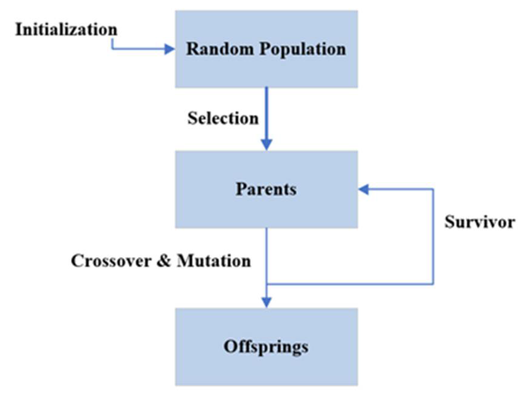
:1. Introduction
1.1. GA Operands
- Selection: This operand determines which chromosomes of the population are selected for reproduction. If a chromosome fits better, it is more likely to be selected for reproduction.
- Crossover: This operator exchanges the subsequences between two chromosomes before and after a locus that is randomly chosen to create two offspring [3].
1.2. Single–Point Crossover
1.3. N-Point Crossover
1.4. Uniform Crossover
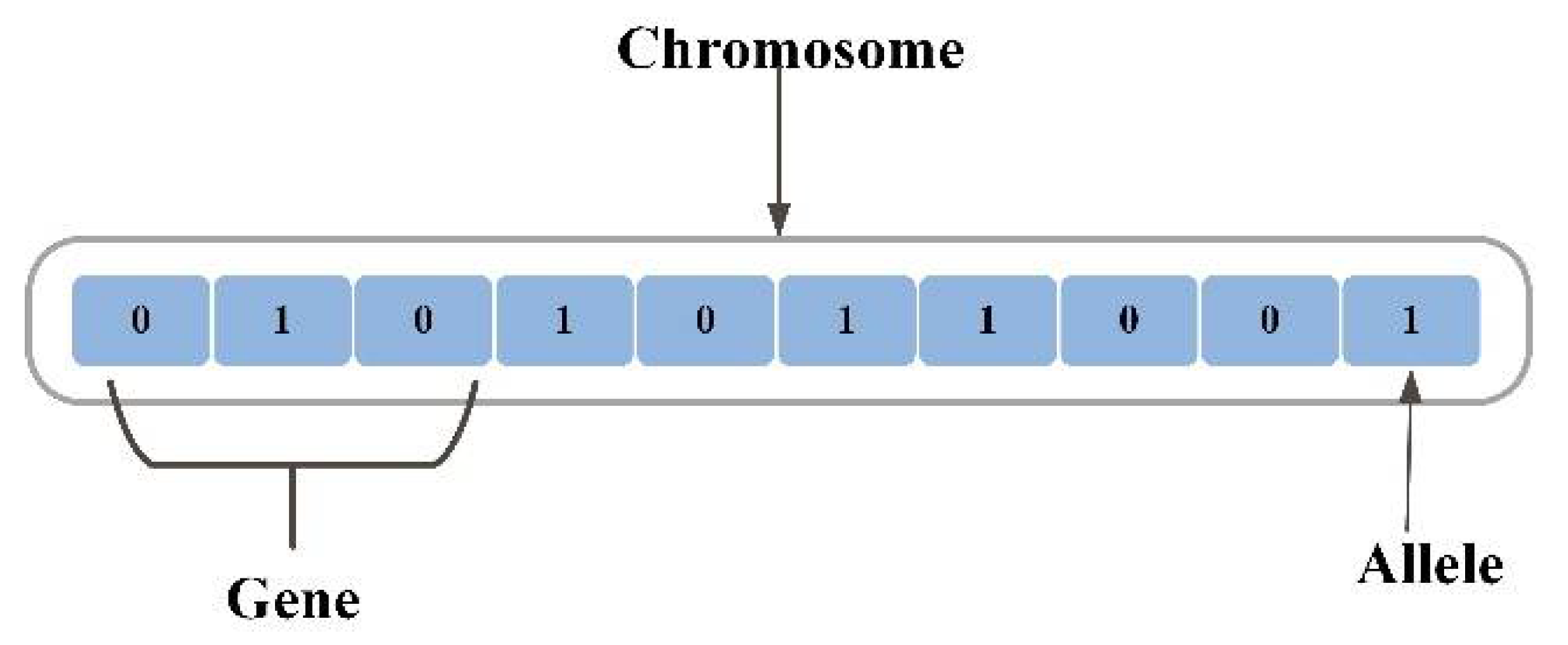
1.5. Numerical Chromosome Representation
1.6. Operators Definition
2. Related Works
2.1. Original Theories
2.2. Implementation of GA
2.3. Optimization in Fields of Science
3. Area of the Proposed Work
3.1. Applications of the Proposed Work
3.2. Minimal-Cost Network Flow
4. System Setup and Main Definitions
- Step 1: Start
- Step 2: Initialize each n population of chromosomes randomly
- Step 3: Generate random mutation ( )
- Step 4: If is = +ve
- Step 5: Else If is = -ve
- Step 6:
- Step 7: End.
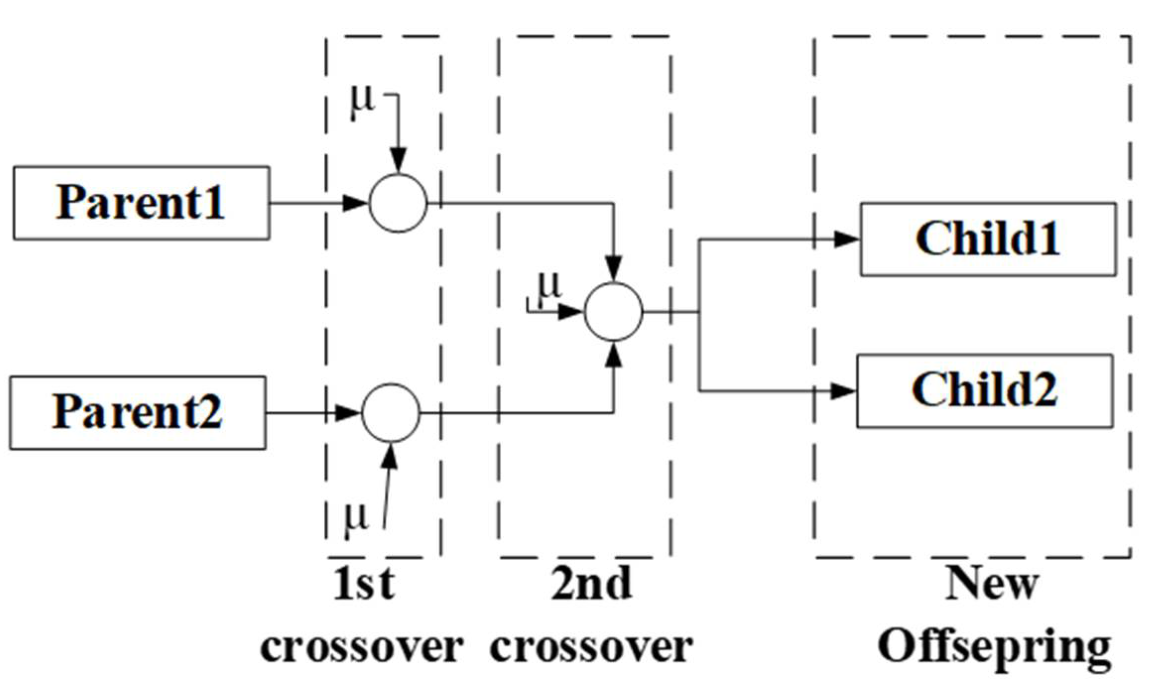
5. Oriented Crossover (OC)
5.1. First Crossover
5.1.1. Binary Crossover
5.1.2. Numerical Crossover
5.2. Second Crossover
6. Experimental Designs
6.1. Optimization Procedure
- Step 1: Initialization for population chromosomes starts by generating random individuals as initialization, each individual’s chromosome with ten “A” attitude alleles for each, as proposed in Section 4.
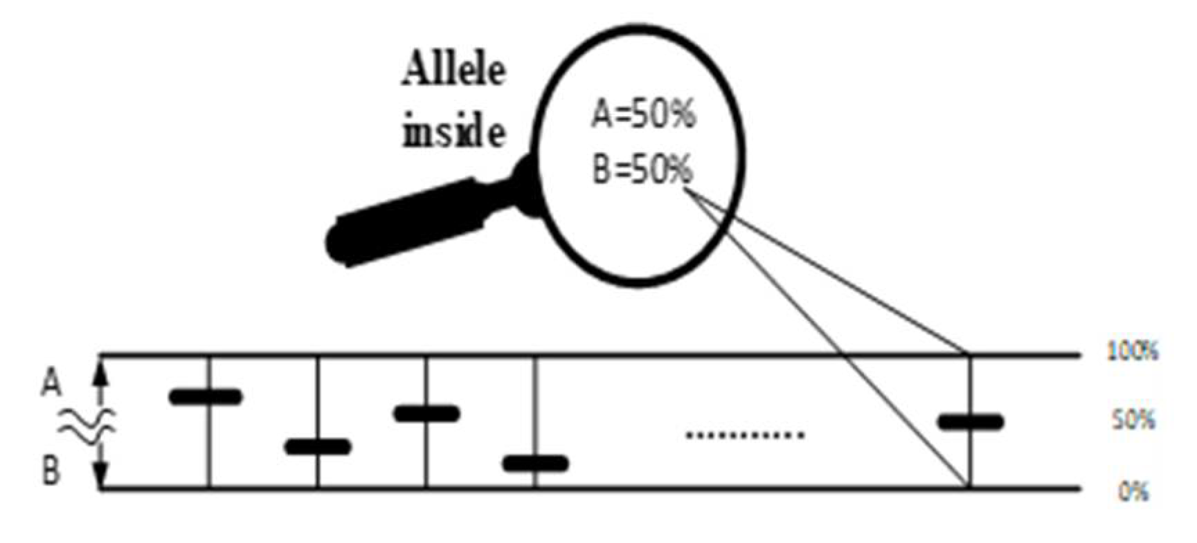
- Step 2: The range of A is [0, 1] for binary crossover, and from 0.1 to 0.9 for each allele in the numerical crossover.
- Step 3: Take the complements of A for each allele to generate the B allele, as discussed in Section 4 of this article.
- Step 4: Calculating the cost function for each parent depends on which equation that needs to be optimized.
- Step 5: Generate and test four isolated populations using Equations (8)–(11) for binary crossover, and a population for numerical crossover using Equations (17) and (18).
- Step 6: Apply the optimization in Equations (19)–(22) as a cost function for each parent in the population with each scenario.
6.2. General Optimization Test
6.3. Communication and Network Optimization
- Step 1: Optimize the parameters in computer networks as per Equations (21) and (22), which leads to minimizing the value of F.
- Step 2: Choose ten individuals to represent the first generation and then calculate the fitness of this generation or Generation Fitness ( as per Equation (23).
- Step 3: Calculate the probability for each individual as per Equation (25).
- Step 4: After arranging the individuals in decreasing order based on their probabilities, eliminate the last two individuals (the two with the least probabilities).
- Step 5: After eliminating two individuals, it now has the best parents ready to mate; thus, it makes the crossover according to the proposed OC algorithm to get new offspring as a new generation.
- Step 6: Repeat the steps from (2) to (6) again till they reach only two individuals in the offspring.
- Step 7: Repeat steps (1) to (7) for one hundred iterations to choose optimal values.
- Step 8: The steps from (1) to (8) are implemented using Equations (19)–(22).
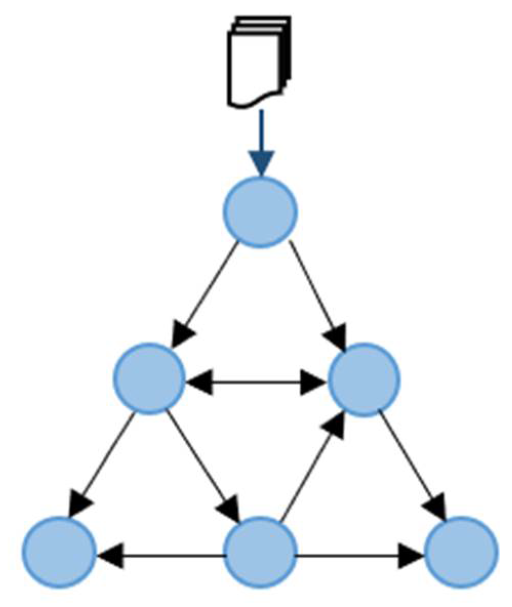
6.4. Fractal-Based WSN Optimization
- General formula for nodes numbers is:
- General formula for the number of links (edges) is:
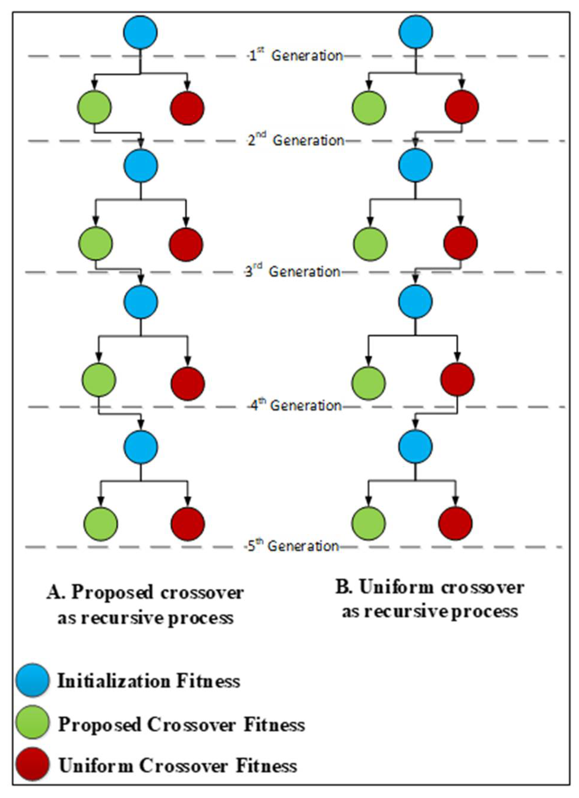
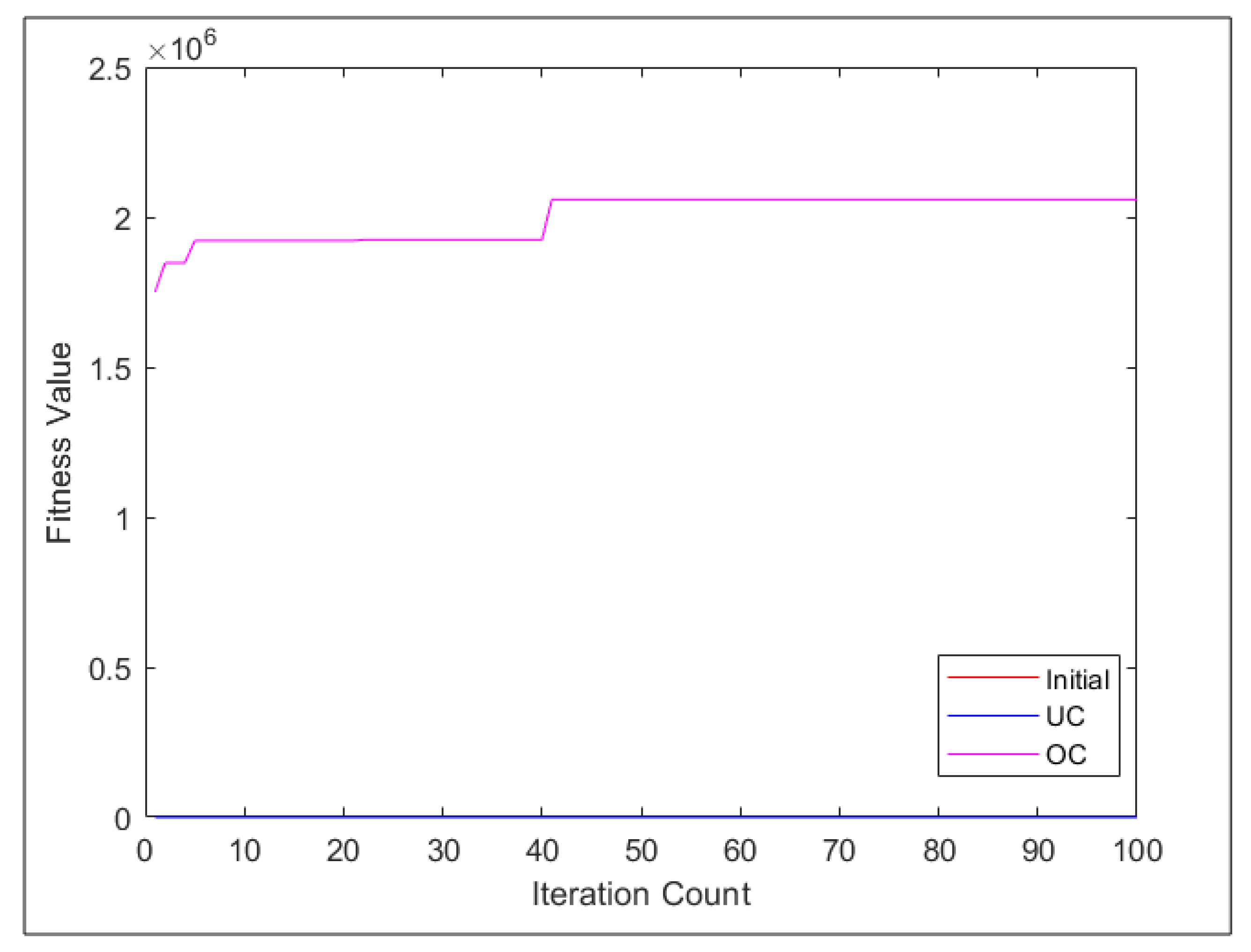
6.5. Recursive Process for Fitness
6.6. Implementation Phases
- Phase one: this phase implements the proposed optimization approach with one type of crossover, which is UC.
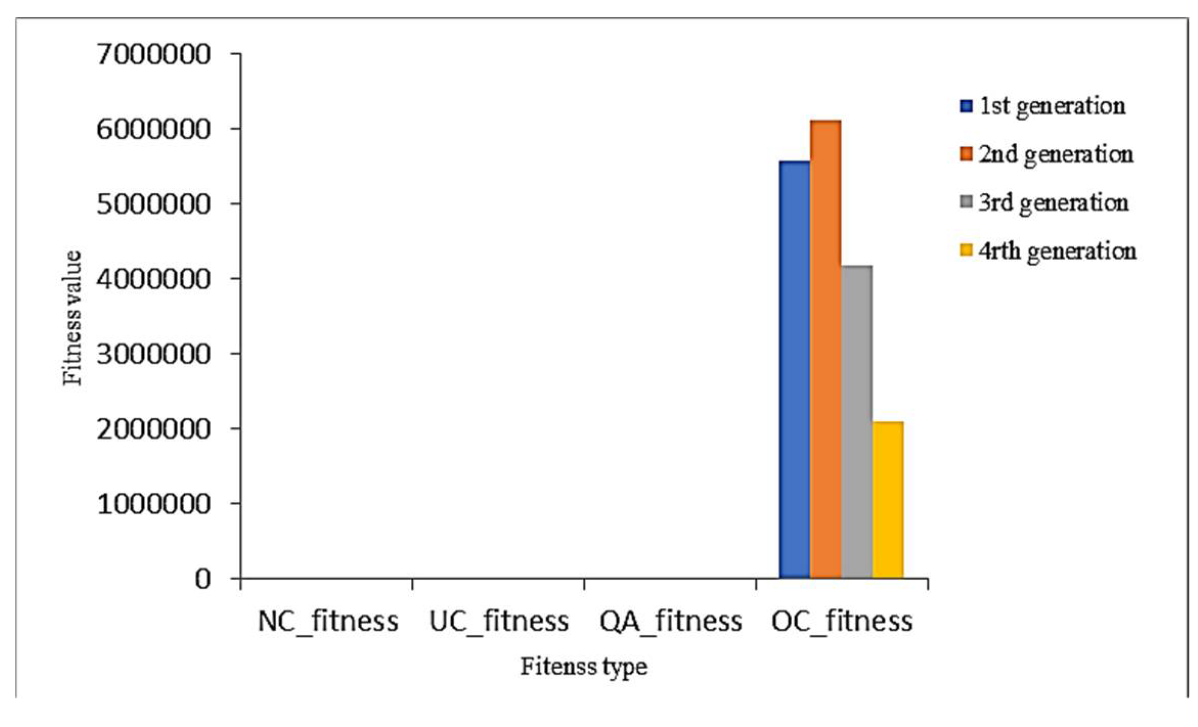
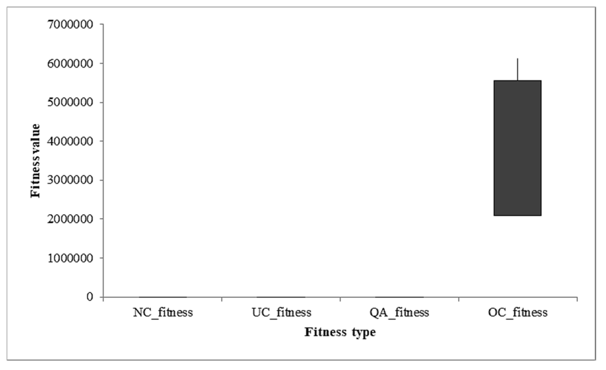
- Phase two: this phase implements the proposed optimization comparatively using UC, NC (with different values of N), and QA [19].
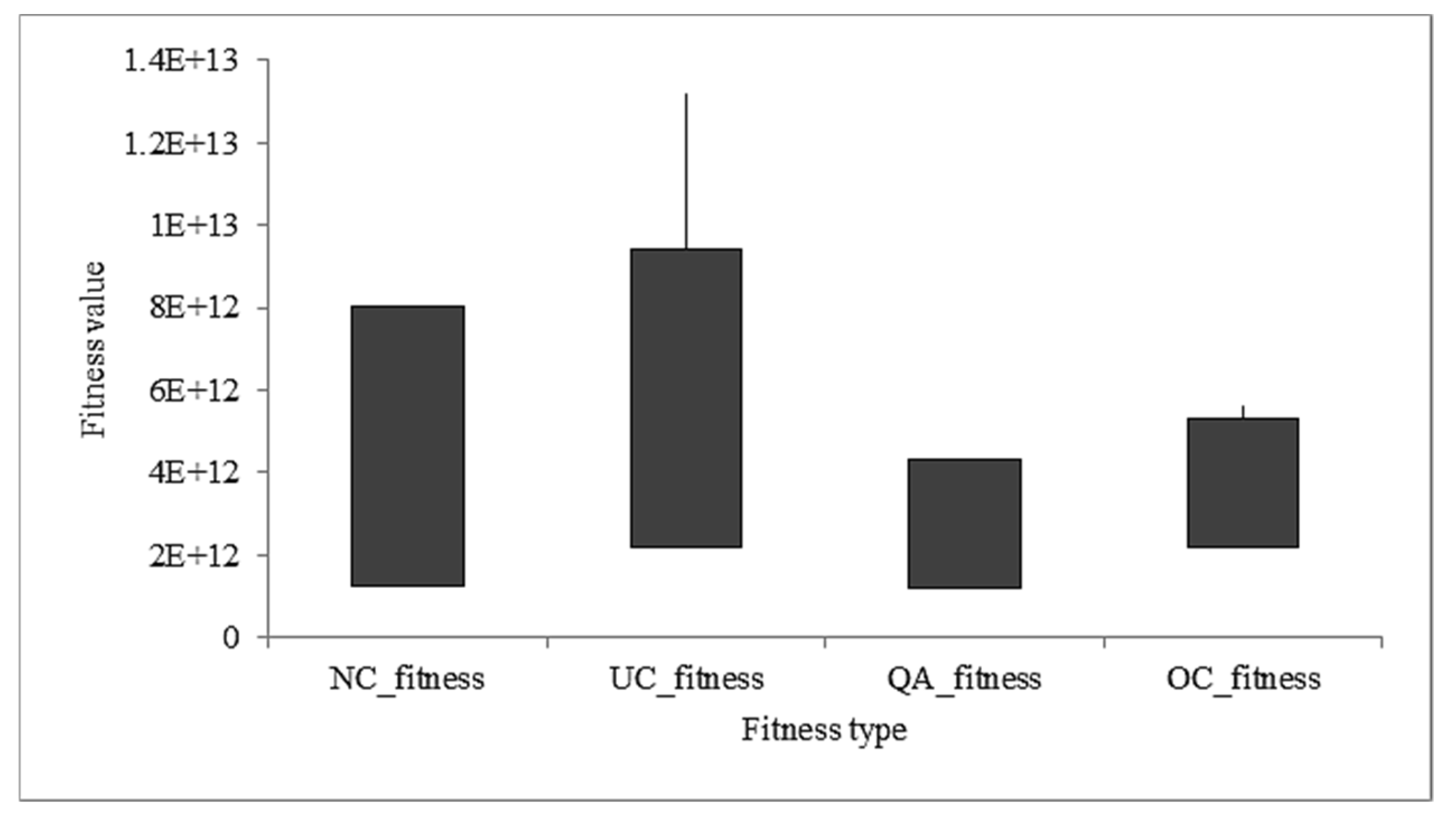
7. Results and Discussion
7.1. Genetic Algorithm Parameters
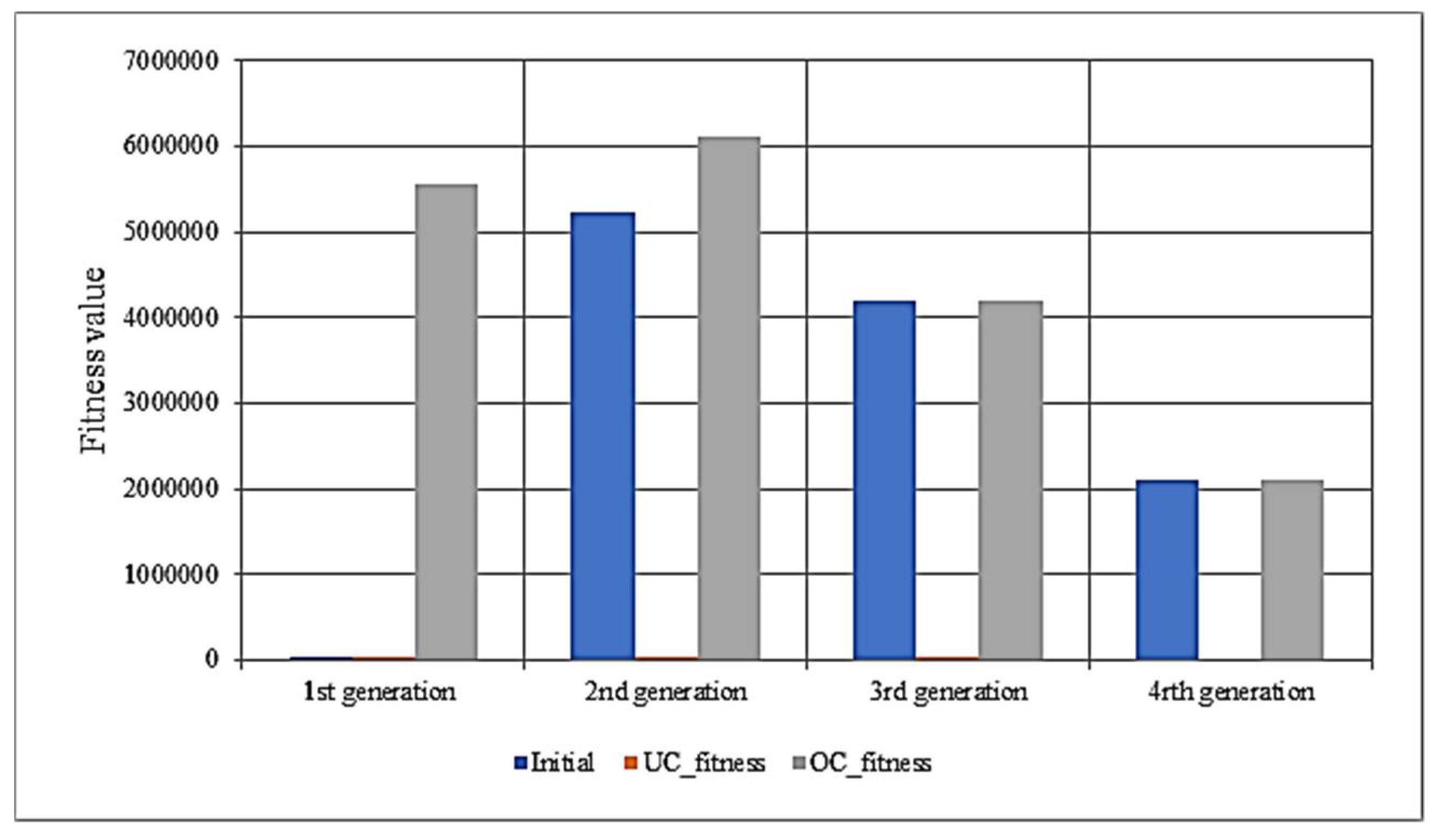
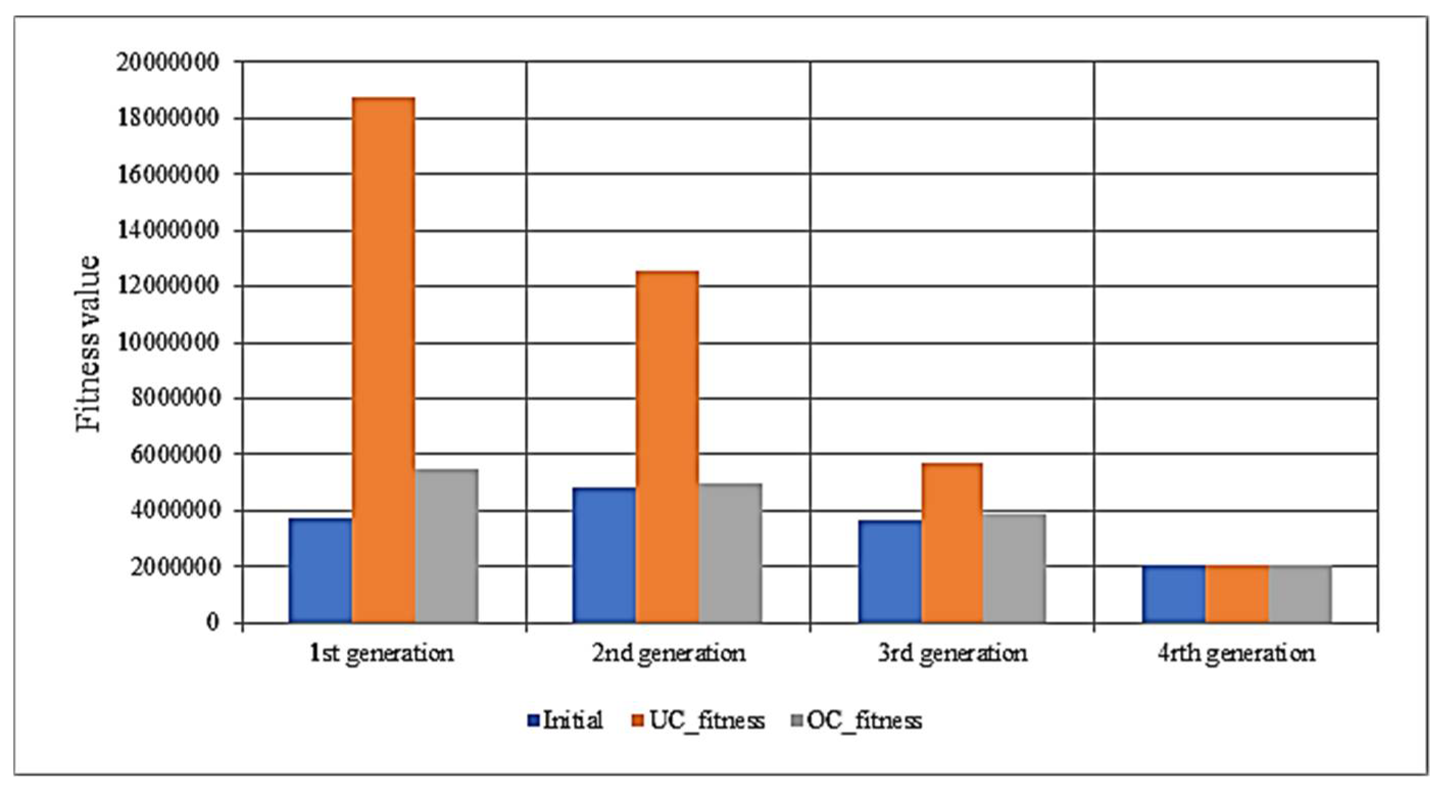
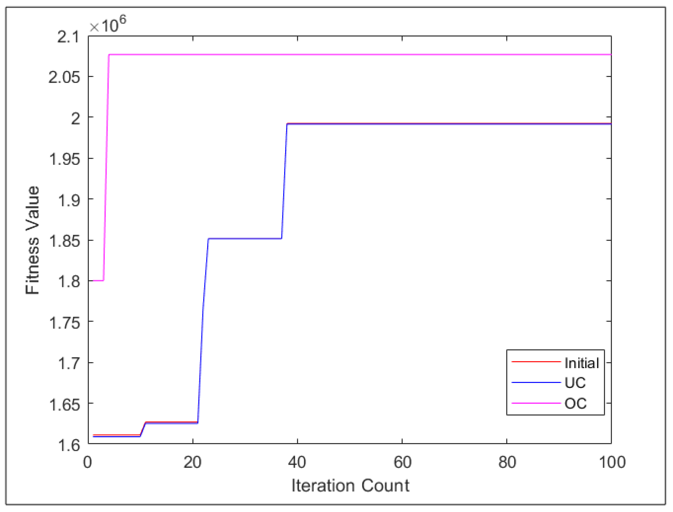
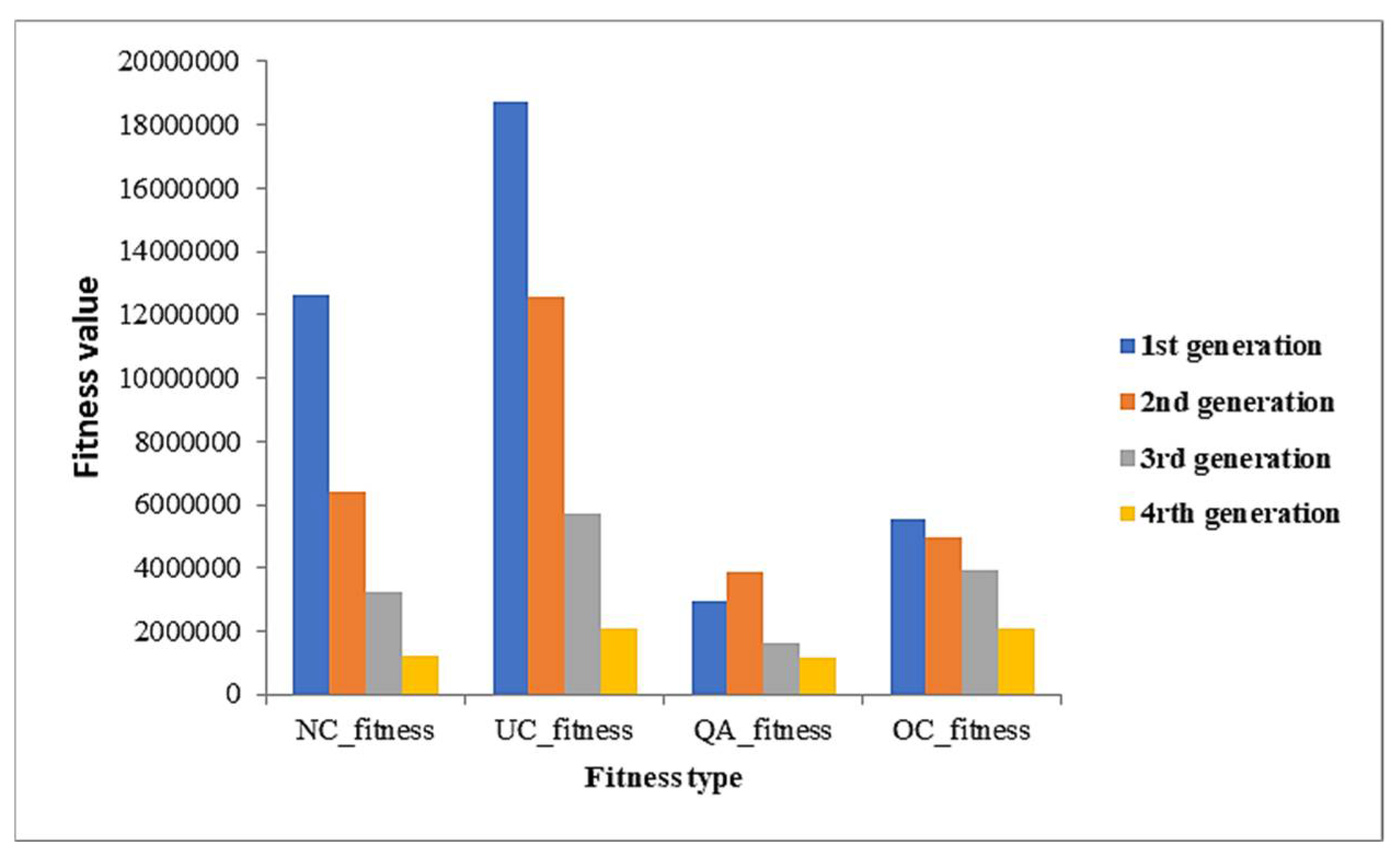
7.2. Binary Crossover under Phase One
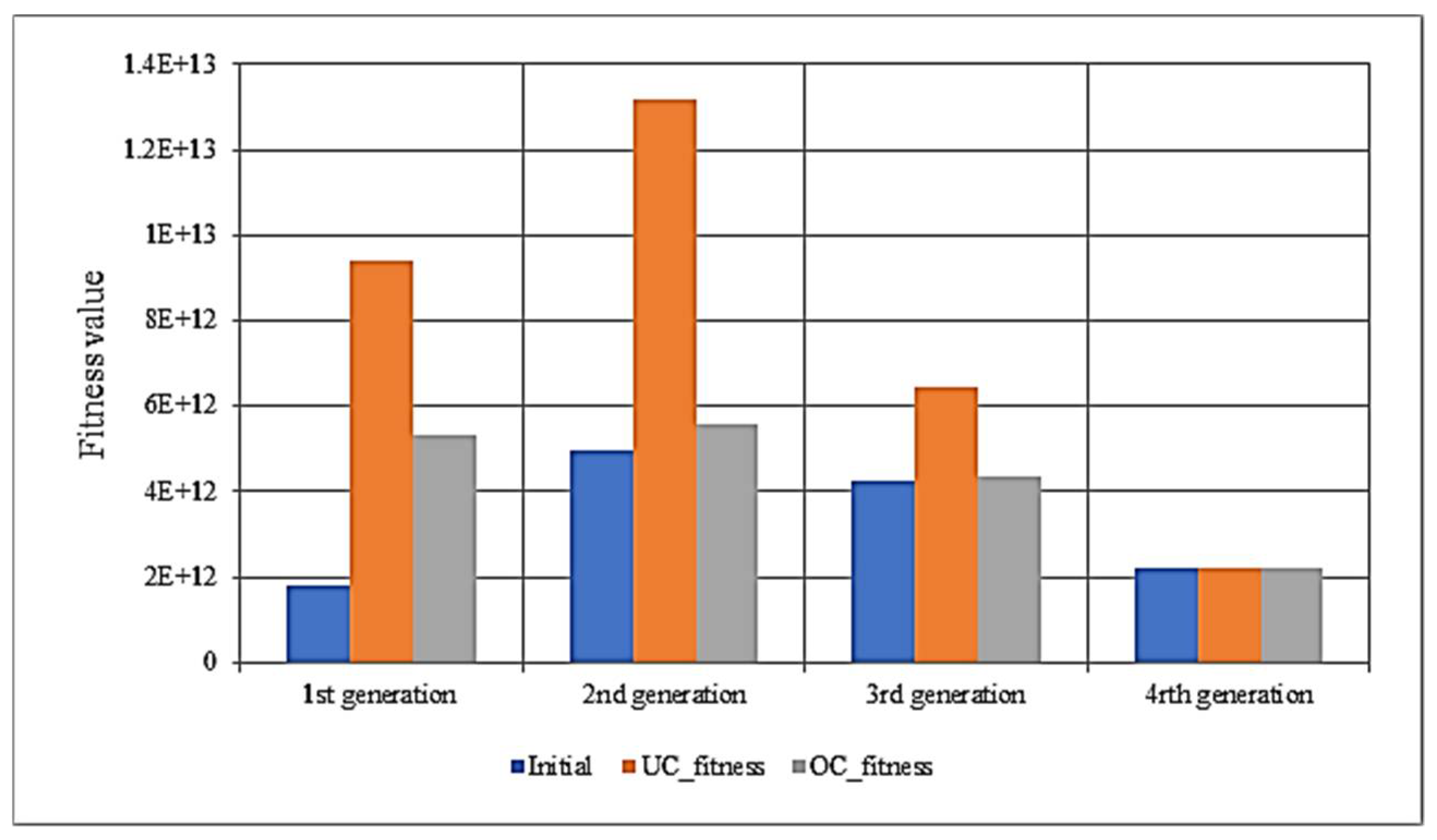
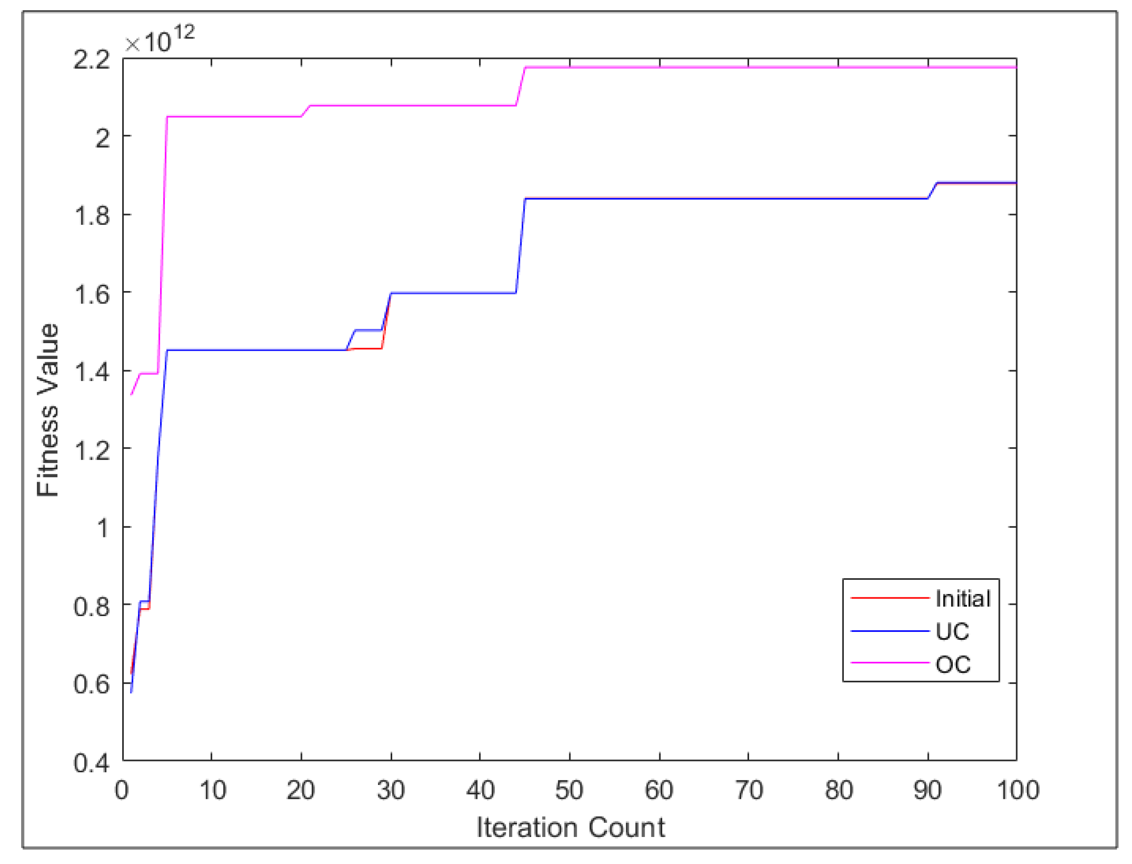
7.3. Numerical Crossover under Phase One
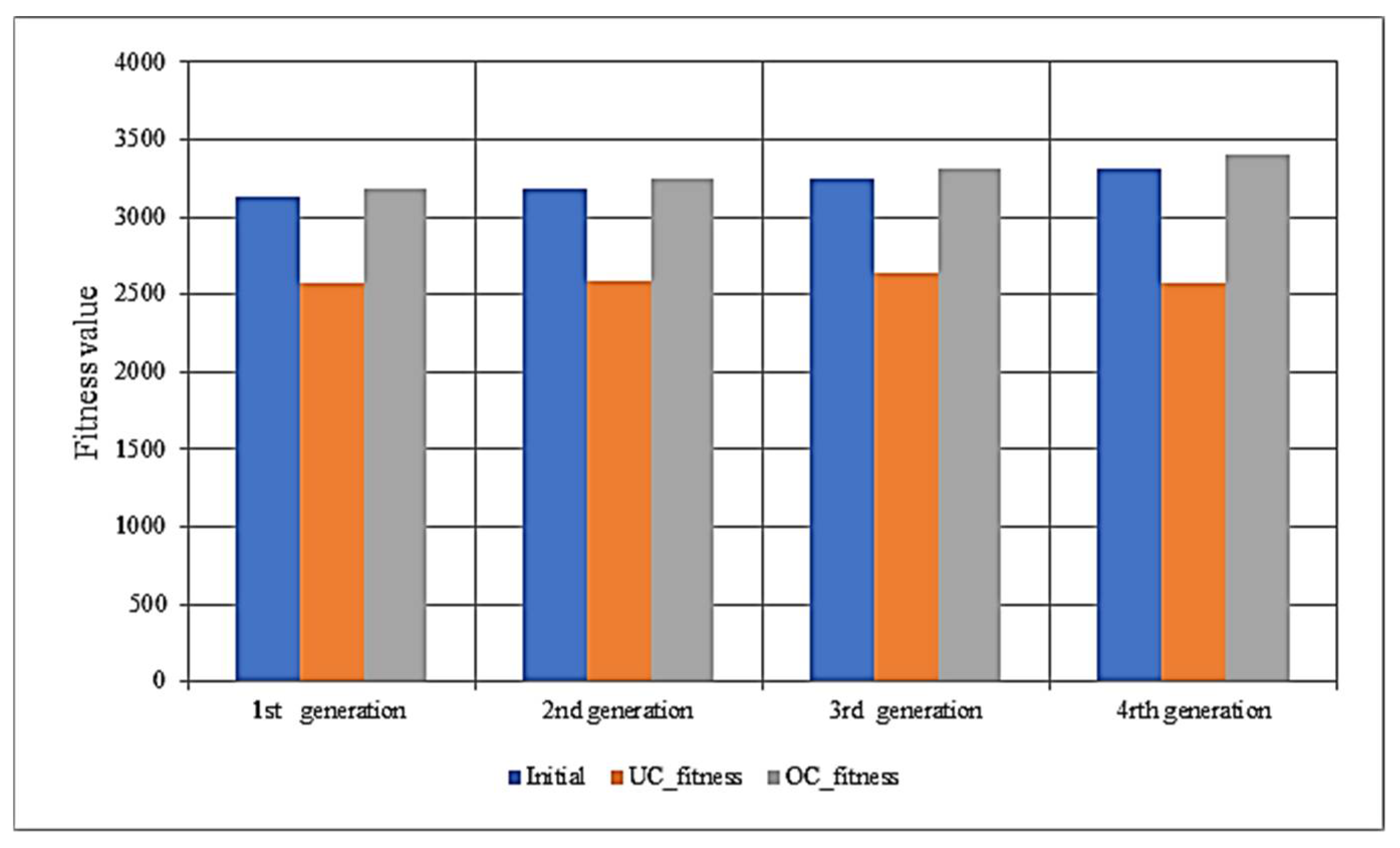
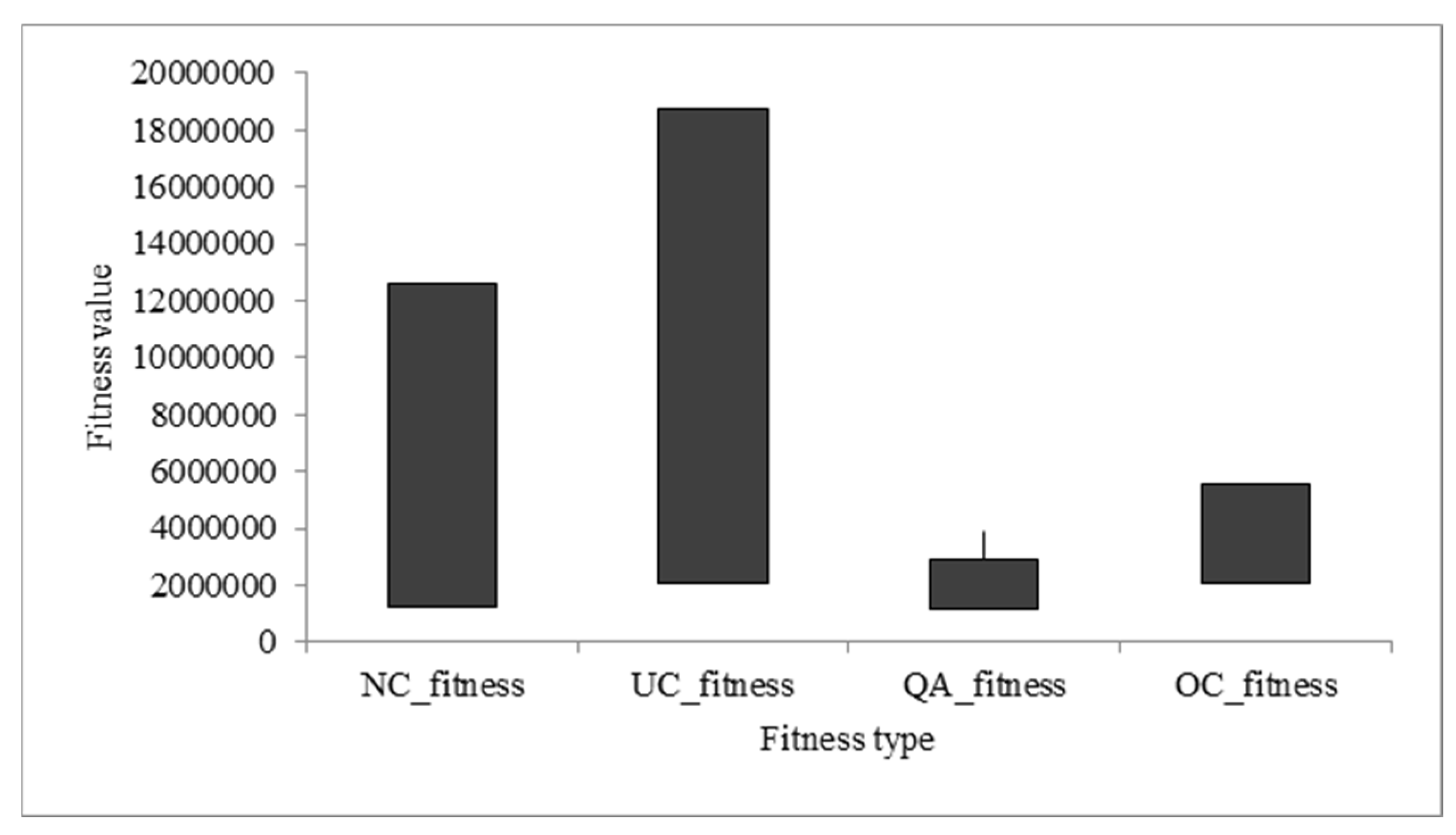
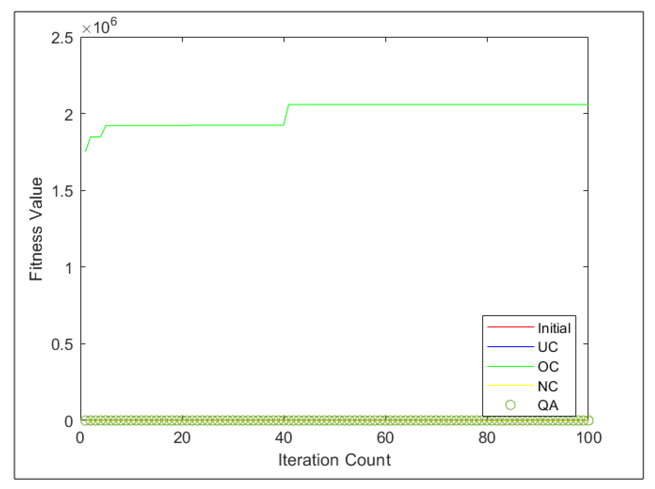
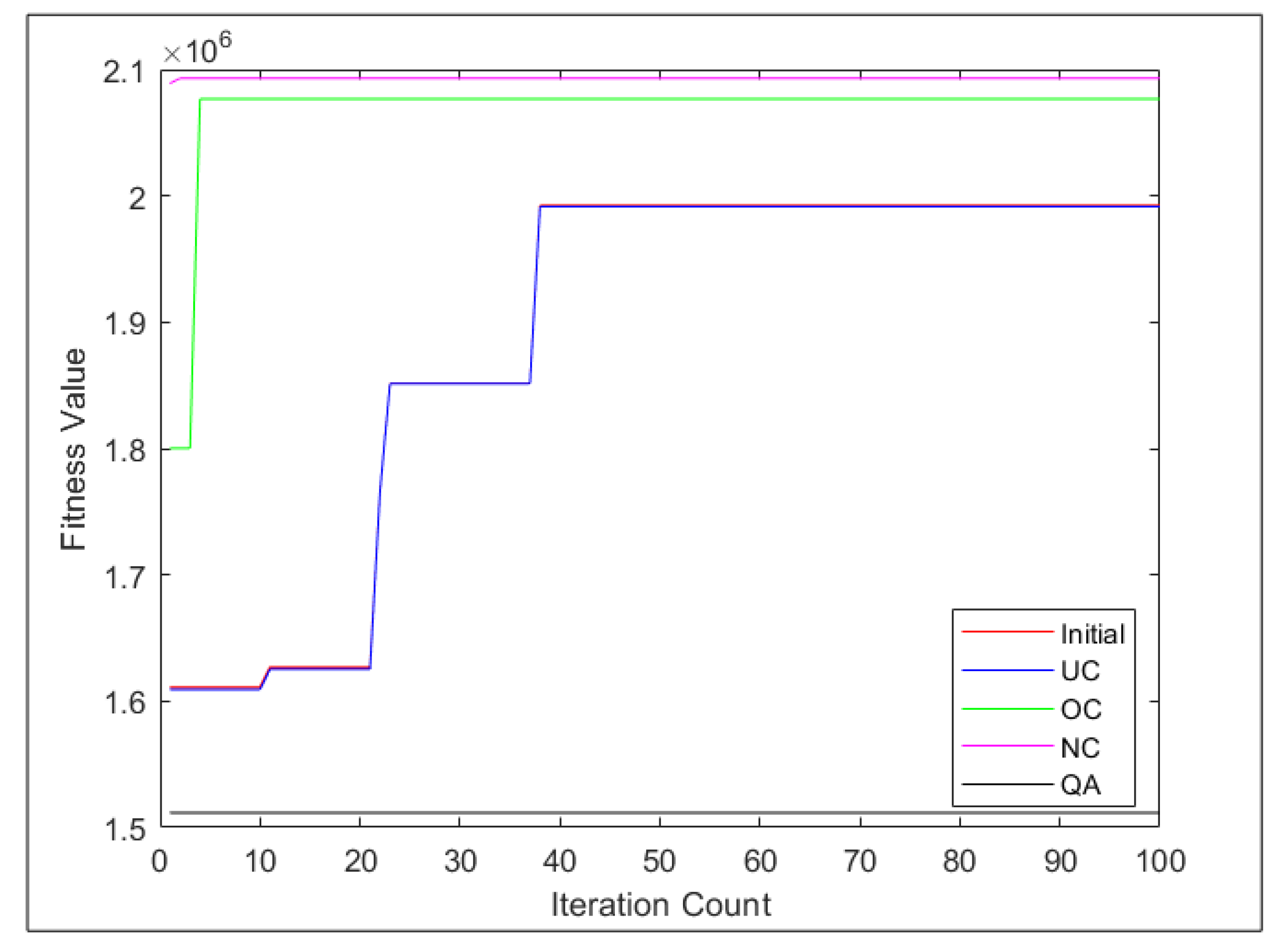
7.4. Equilibrium State under Phase One
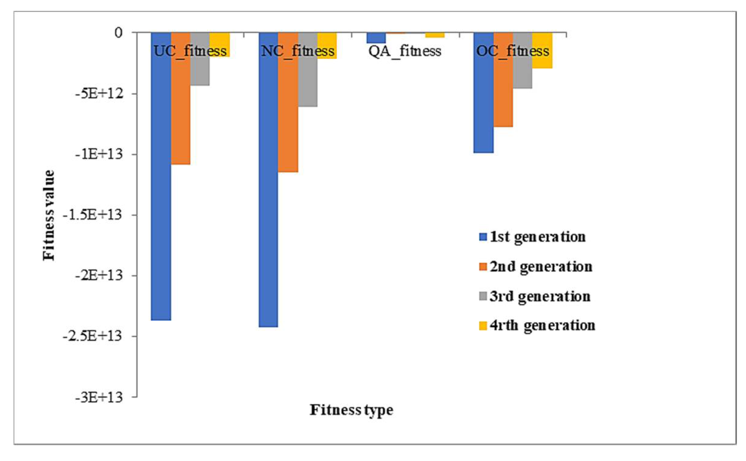
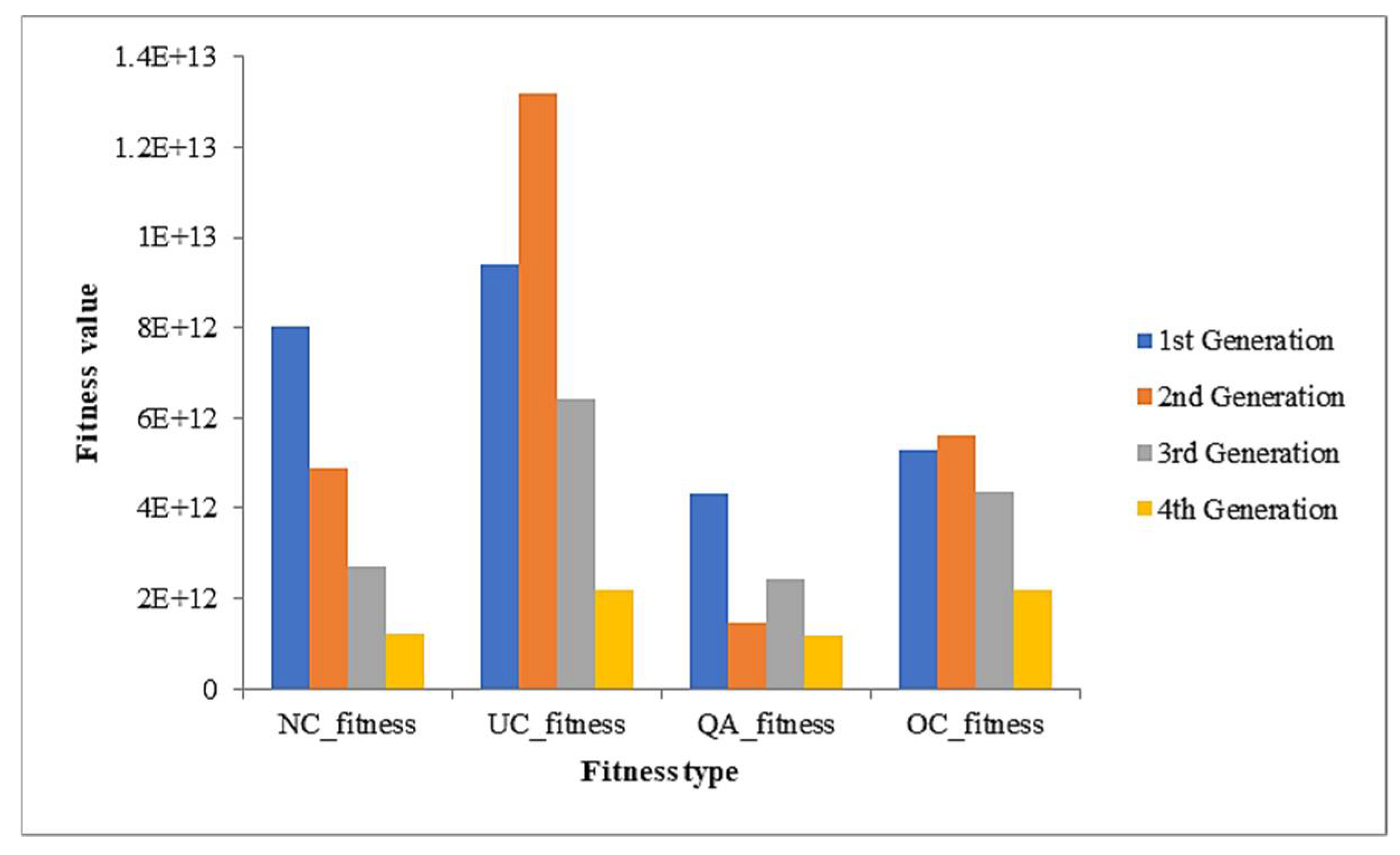
7.5. Binary Crossover under Phase Two
7.6. Numerical Crossover under Phase Two
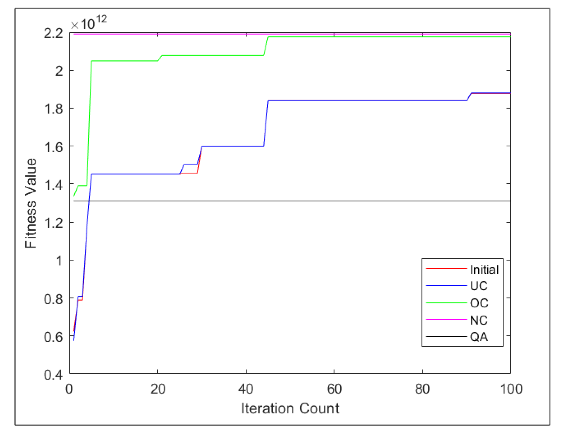
7.7. Equilibrium State under Phase Two
8. Concluding Remarks
Author Contributions
Funding
Data Availability Statement
Acknowledgments
Conflicts of Interest
References
- Kora, P.; Yadlapalli, P. Crossover operators in genetic algorithms: A review. Int. J. Comput. Appl. 2017, 162, 34–36. [Google Scholar] [CrossRef]
- Hussain, A.; Muhammad, Y.S.; Sajid, M.N. An Efficient Genetic Algorithm for Numerical Function Optimization with Two New Crossover Operators. Int. J. Math. Sci. Comput. 2018, 4, 41–55. [Google Scholar] [CrossRef]
- Mitchell, M. An Introduction to Genetic Algorithms; MIT Press: Cambridge, MA, USA, 1998. [Google Scholar]
- Chiroma, H.; Abdulkareem, S.; Abubakar, A.; Herawan, T. Neural networks optimization through genetic algorithm searches: A review. Appl. Math. Inf. Sci. 2017, 11, 1543–1564. [Google Scholar] [CrossRef]
- Manzoni, L.; Mariot, L.; Tuba, E. Balanced crossover operators in genetic algorithms. Swarm Evol. Comput. 2020, 54, 100646. [Google Scholar] [CrossRef]
- Holland, J.H. Adaptation in Natural and Artificial Systems; University of Michigan Press: Ann Arbor, MI, USA, 1975. [Google Scholar]
- Spears, W. Adapting Crossover in a Genetic Algorithm; Technical Report; Naval Research Laboratory: Washington, DC, USA, 1994. [Google Scholar]
- Syswerda, G. Uniform Crossover in Genetic Algorithms. In Proceedings of the 3rd International Conference on Genetic Algorithms, Fairfax, VA, USA, 2–9 June 1989; Morgan Kaufmann Publishers Inc., 340 Pine Street: San Francisco, CA, USA, 1989. [Google Scholar]
- Umbarkar, A.J.; Sheth, P.D. Crossover operators in genetic algorithms: A review. ICTACT J. Soft Comput. 2015, 6, 1083–1092. [Google Scholar]
- Sivanandam, S.; Deepa, S. Genetic Algorithms. In Introduction to Genetic Algorithms; Springer: Berlin/Heidelberg, Germany, 2008; pp. 15–37. [Google Scholar]
- Kirchner-Bossi, N.; Porté-Agel, F. Realistic wind farm layout optimization through genetic algorithms using a Gaussian wake model. Energies 2018, 11, 3268. [Google Scholar] [CrossRef]
- Félix Patrón, R.S.; Botez, R.M. Flight trajectory optimization through genetic algorithms coupling vertical and lateral profiles. In Proceedings of the ASME International Mechanical Engineering Congress and Exposition, Montreal, QC, Canada, 14–20 November 2014; p. 46421. [Google Scholar]
- Bani-Hani, D.; Khan, N.; Alsultan, F.; Karanjkar, S.; Nagarur, N. Classification of leucocytes using convolutional neural network optimized through genetic algorithm. In Proceedings of the 7th Annual World Conference of the Society for Industrial and Systems Engineering, Binghamton, NY, USA, 11–12 October 2018. [Google Scholar]
- Zeidabadi, F.A.; Dehghani, M. Poa: Puzzle optimization algorithm. Int. J. Intell. Eng. Syst. 2022, 15, 273–281. [Google Scholar]
- Anju, K.; Avanish, K. An advanced approach to the employee recruitment process through genetic algorithm. Int. J. Inf. Technol. 2021, 13, 313–319. [Google Scholar] [CrossRef]
- Begum, S.; Padmannavar, S.S. Genetically Optimized Ensemble Classifiers for Multiclass Student Performance Prediction. Int. J. Intell. Eng. Syst. 2022, 15, 316–328. [Google Scholar]
- Haldulakar, R.; Agrawal, J. Optimization of association rule mining through genetic algorithm. Int. J. Comput. Sci. Eng. (IJCSE) 2011, 3, 1252–1259. [Google Scholar]
- Muthana, S.A.; Ku-Mahamud, K.R. Comparison of Multi-objective Optimization Methods for Generator Maintenance Scheduling. Methods (Multi-Object. Metaheuristics) 2022, 14, 15. [Google Scholar]
- Rabee, F.; Jazaery, I.; Kumar, K. Quaternary-Child Crossover for Genetic Algorithm in Real-Time Scheduling Optimization. Int. J. Intell. Eng. Syst. 2023, 16, 100–114. [Google Scholar]
- Abdulkadhim, F.G.; Yi, Z.; Onaizah, A.N.; Rabee, F.; Al-Muqarm AM, A. Optimizing the Roadside Unit Deployment Mechanism in VANET with Efficient Protocol to Prevent Data Loss. Wirel. Pers. Commun. 2022, 127, 815–843. [Google Scholar] [CrossRef]
- Lu, F.; Bi, H.; Huang, M.; Duan, S. Simulated Annealing Genetic Algorithm Based Schedule Risk Management of IT Outsourcing Project. Math. Probl. Eng. 2017, 2017, 6916575. [Google Scholar] [CrossRef]
- Pandey, H.M.; Chaudhary, A.; Mehrotra, D. Grammar induction using bit masking oriented genetic algorithm and comparative analysis. Appl. Soft Comput. 2016, 38, 453–468. [Google Scholar] [CrossRef]
- Bi, H.; Lu, F.; Duan, S.; Huang, M.; Zhu, J.; Liu, M. Two-level principal–agent model for schedule risk control of IT outsourcing project based on genetic algorithm. Eng. Appl. Artif. Intell. 2020, 91, 103584. [Google Scholar] [CrossRef]
- Yan, T.; Lu, F.; Wang, S.; Wang, L.; Bi, H. A hybrid metaheuristic algorithm for the multi-objective location-routing problem in the early post-disaster stage. J. Ind. Manag. Optim. 2022, 19, 4663–4691. [Google Scholar] [CrossRef]
- Abdul-Sada, H.H.; Rabee, F. The Genetic Algorithm Implementation in Smart Contract for the Blockchain Technology. Al-Salam J. Eng. Technol. 2023, 2, 37–47. [Google Scholar]
- Singh, J. An Optimal Resource Provisioning Scheme Using QoS in Cloud Computing Based Upon the Dynamic Clustering and Self-Adaptive Hybrid Optimization Algorithm. Int. J. Intell. Eng. Syst. 2022, 15, 148–160. [Google Scholar]
- Sanapala, R.K.; Duggirala, S.R. An Optimized Energy Efficient Routing for Wireless Sensor Network using Improved Spider Monkey Optimization Algorithm. Transportation 2022, 8, 9. [Google Scholar]
- Jubair, A.M.; Hassan, R.; Aman, A.H.; Sallehudin, H.; Al-Mekhlafi, Z.G.; Mohammed, B.A.; Alsaffar, M.S. Optimization of Clustering in Wireless Sensor Networks: Techniques and Protocols. Appl. Sci. 2021, 11, 11448. [Google Scholar] [CrossRef]
- Rangappa, M.H.; Dyamanna, G.C. Energy-Efficient Routing Protocol for Hybrid Wireless Sensor Networks Using Falcon Optimization Algorithm. Int. J. Intell. Eng. Syst. 2022, 15, 1–10. [Google Scholar]
- Cinat, P.; Gnecco, G.; Paggi, M. Multi-scale surface roughness optimization through genetic algorithms. Front. Mech. Eng. 2020, 6, 29. [Google Scholar] [CrossRef]
- Forouzan, B.A. TCP/IP Protocol Suite, 4th ed.; McGraw-Hill Higher Education: New York, NY, USA, 2010. [Google Scholar]
- Singh, N.; Chaurasia, P. A Review on Genetic Algorithm Operations and Application in Telecommunication Routing. Int. J. Comput. Sci. Eng. 2019, 7, 273–277. [Google Scholar] [CrossRef]
- Kwon, C. Julia Programming for Operations Research 2022, 2nd ed.; University of South Florida: Tampa, FL, USA, 2022. [Google Scholar]
- Schärfe, C.P.I.; Tremmel, R.; Schwab, M.; Kohlbacher, O.; Marks, D.S. Genetic variation in human drug-related genes. Genome Med. 2017, 9, 117. [Google Scholar] [CrossRef]
- King, E.A.; Davis, J.W.; Degner, J.F. Are drug targets with genetic support twice as likely to be approved? Revised estimates of the impact of genetic support for drug mechanisms on the probability of drug approval. PLoS Genet. 2019, 15, e1008489. [Google Scholar] [CrossRef]
- Ortiz-Boyer, D.; Hervás-Martínez, C.; Garcia-Pedrajas, N. Cixl2: A crossover operator for evolutionary algorithms based on population features. J. Artif. Intell. Res. 2005, 24, 1–48. [Google Scholar] [CrossRef]
- Li, X.; Engelbrecht, A.; Epitropakis, M.G. Benchmark Functions for CEC’2013 Special Session and Competition on Niching Methods for Multimodal Function Optimization; Evolutionary Computation and Machine Learning Group, Australia, Tech. Rep., RMIT University: Melbourne, Australia, 2013. [Google Scholar]
- Khudhair, M.M.; Adil, A.R.; Rabee, F. An innovative fractal architecture model for implementing MapReduce in an open multiprocessing parallel environment. Indones. J. Electr. Eng. Comput. Sci. 2023, 30, 1059–1067. [Google Scholar]
- Khudhair, M.M.; Rabee, F.; AL-Rammahi, A. New efficient fractal models for MapReduce in OpenMP parallel environment. Bull. Electr. Eng. Inform. 2023, 12, 2313–2327. [Google Scholar] [CrossRef]


| Parameters | Value per Population | Factor |
|---|---|---|
| Population Size | 10 | ×12 |
| Scaling Function for selection probability | Uniform distribution | ……… |
| Selection Operator | Roulette Wheel | ……… |
| Crossover Probability | 80% | ×12 |
| Mutation Operator | OR | ……… |
| Mutation Probability | 10% | ……… |
Disclaimer/Publisher’s Note: The statements, opinions and data contained in all publications are solely those of the individual author(s) and contributor(s) and not of MDPI and/or the editor(s). MDPI and/or the editor(s) disclaim responsibility for any injury to people or property resulting from any ideas, methods, instructions or products referred to in the content. |
© 2023 by the authors. Licensee MDPI, Basel, Switzerland. This article is an open access article distributed under the terms and conditions of the Creative Commons Attribution (CC BY) license (https://creativecommons.org/licenses/by/4.0/).
Share and Cite
Rabee, F.; Hussain, Z.M. Oriented Crossover in Genetic Algorithms for Computer Networks Optimization. Information 2023, 14, 276. https://doi.org/10.3390/info14050276
Rabee F, Hussain ZM. Oriented Crossover in Genetic Algorithms for Computer Networks Optimization. Information. 2023; 14(5):276. https://doi.org/10.3390/info14050276
Chicago/Turabian StyleRabee, Furkan, and Zahir M. Hussain. 2023. "Oriented Crossover in Genetic Algorithms for Computer Networks Optimization" Information 14, no. 5: 276. https://doi.org/10.3390/info14050276