Article

Structure Learning and Hyperparameter Optimization Using an Automated Machine Learning (AutoML) Pipeline

by
Konstantinos Filippou
1,
George Aifantis
1,
George A. Papakostas
2 and
George E. Tsekouras
1,*
1
Computational Intelligence (CI) Research Group, Department of Cultural Technology and Communications, University of the Aegean, 81100 Mytilene, Greece
2
MLV Research Group, Department of Computer Science, International Hellenic University, 65404 Kavala, Greece
*
Author to whom correspondence should be addressed.
Information 2023, 14(4), 232; https://doi.org/10.3390/info14040232
Submission received: 14 February 2023 / Revised: 22 March 2023 / Accepted: 6 April 2023 / Published: 9 April 2023
(This article belongs to the Special Issue Systems Engineering and Knowledge Management)

Abstract

:
In this paper, we built an automated machine learning (AutoML) pipeline for structure-based learning and hyperparameter optimization purposes. The pipeline consists of three main automated stages. The first carries out the collection and preprocessing of the dataset from the Kaggle database through the Kaggle API. The second utilizes the Keras-Bayesian optimization tuning library to perform hyperparameter optimization. The third focuses on the training process of the machine learning (ML) model using the hyperparameter values estimated in the previous stage, and its evaluation is performed on the testing data by implementing the Neptune AI. The main technologies used to develop a stable and reusable machine learning pipeline are the popular Git version control system, the Google cloud virtual machine, the Jenkins server, the Docker containerization technology, and the Ngrok reverse proxy tool. The latter can securely publish the local Jenkins address as public through the internet. As such, some parts of the proposed pipeline are taken from the thematic area of machine learning operations (MLOps), resulting in a hybrid software scheme. The machine learning model was used to evaluate the pipeline, which is a multilayer perceptron (MLP) that combines typical dense, as well as polynomial, layers. The simulation results show that the proposed pipeline exhibits a reliable and accurate performance while managing to boost the network’s performance in classification tasks.

1. Introduction

Automated machine learning (AutoML) is a rapidly growing field that exemplifies the systematic and automated development and deployment of machine learning (ML) tools [1,2]. The impetus to the wide spread of AutoML techniques was given by the need to avoid manual interference (i.e., trial-and-error choices) in model’s design, which have been recognized as a time-consuming procedure, without giving guarantee for the ML model’s accurate performance [3,4]. In the framework of AutoML, the model’s creation becomes easier, in the sense that it requires a minimal (or at the best scenario not at all) designer’s manual correction. As a result, it can be viewed as an alternative to more traditional considerations [5,6], operating as a vehicle, to alleviate the high demands for experts in building ML applications [7]; this is a fact that appears to be very appealing in commercial software production [8]. In addition, under the umbrella of AutoML, the ML approaches become accessible to non-expert users [9], thus enabling the organizations to leverage the power of ML in effectively solving a variety of real-world problems [1].
So far, several libraries have been designed to perform AutoML procedures. Among others, we can mention the Auto-Weka [10], Auto-Keras [11], Auto-Pytorch [12], Auto-Sklearn [13], etc. In addition, AutoML structures have been used over a wide range of applications, such as classification [14,15], regression analysis [16], remote sensing [17], cyber-security and privacy [18,19], medical applications [20], web-based applications [21], time-series analysis [22], etc.
The basic philosophical idea behind AutoML techniques is the simultaneous training of several models over the same data set, and then we select the best one, based on establishing an effective evaluation strategy [23,24]. Overall, this encircles several stages applied in sequence, which are shown in Figure 1.
The first stage concerns the data preprocessing and is carried out in terms of [4,8,22,23,25]: (a) data collection approaches that generate a proper data set to train an ML model, (b) data visualization techniques, which are employed to assist the data analyst in comprehending the internal data structure, (c) data cleaning mechanisms that eliminate the noise existing in the available data set and avoid the creation of compromised models, and (d) data augmentation procedures that are used to extend the original data set and enhance the model’s robustness by avoiding overfitting problems. The second stage uses feature engineering mechanisms to extract features from the raw data and to make more convenient the design of ML algorithms in effectively describing the data [4]. Mainly, it is projected on: (a) feature selection algorithms that act to reject features from the original feature set, which appear to be redundant, or they deteriorate the model’s performance [8], and (b) feature extraction methods that perform dimensionality reduction using specialized functional data transformations thus, altering the original data features [4,9]. The third stage concerns the model generation and is recognized as the very core of an AutoML approach. Model generation is performed in terms of two processes, namely, structure identification and architecture optimization [4,9]. Structure identification concerns the determination of the ML approach that best solves the problem at hand. Typical structures commonly used are neural networks or deep neural networks [4,9,25]. The next process is to optimize the architecture and the set of hyperparameters (e.g., learning rate, number of layers, etc.) and come up with the best ML model [22,26,27]. The final stage focuses on the assessment of the model’s performance, which can be carried out in terms of well defined performance measures [4,9].
A thematic area close to AutoML concerns the ML Operations (MLOps) practices. MLOps constitute a set of tools and mechanisms able to enhance the collaboration between data scientists and IT professionals in applying and maintaining ML models [28,29]. In turn, MLOps practices are in the position to assist the risk management associated with deploying ML models in production by providing traceability, monitoring, and testing capabilities [28,30,31]. In general, two major issues are considered in designing MLOps procedures [28,30,32]. The first one is related to compatibility problems arising from the fact that MLOps practices integrate a wide range of heterogeneous tools, technologies, and software environments. The second issue reflects on the risks of errors and failures in a software production environment. To reduce the above risks, it is important to perform robust monitoring and testing [4]. The main components that MLOps implementations offer to ML software production are: (a) collaboration and communication, (b) automation and orchestration, and (c) monitoring and testing. The former optimizes the model’s development and deployment in terms of continuous integration and continuous delivery (CI/CD) practices. The latter enhances the production of highly effective and reliable ML models [28,33]. CI/CD mechanisms are very essential in MLOps’ development because they establish real-time model testing and deployment [34]. These mechanisms involve the design of different versions of software frameworks to handle code changes and to create automated testing tools for quality assessment and deploy software automation tools to manage the rollout of the above code changes [35,36], with the ultimate purpose being the automatic production of software applications in a continuous and iterative manner, utilizing less time and effort [34,35,36].
This paper proposes a ML software development pipeline that combines AutoML with MLOps practices to build, tune, validate, and monitor ML models for the test case of data classification problems. The framework is synthesized by a sequence of steps that encompass edge technologies, such as Git version control, Github repository, Jenkins server, Ngrok, and Neptune AI. The ML structures employed are multilayer perceptron (MLP) type of neural networks that involve dense layers, with typical activation functions and layers with Hermite polynomial activation functions, thus resulting in a hybrid network architecture. Certain simulation experiments are carried out to monitor and validate the pipeline.
The rest of the paper consists of the following sections. Section 2 reports the related studies and discusses the novelty of the current contribution. Section 3 presents a detailed analysis of the structure and functionality of the proposed methodology. Section 4 illustrates the experimental results. Finally, the paper concludes in Section 5.

2. Related Studies and the Current Contribution

In recent years, the AutoML thematic area has gained the attention of a growing number of researchers, mainly due to its capability to engage ML algorithms with the systematic software production at the level of organizations and companies that operate on software development. As such, several theoretical and practical results have been acquired so far. In this section, some methodologies, related to the one proposed in this paper, are briefly described and discussed.
One of the most studied applications of AutoML is its usage in classification problems. Singh et al. [20] created a programming environment for classifying various hepatic diseases using ML models. The environment was a software platform synthesized by three libraries, namely, Auto-WEKA [10], Auto-Keras [11], and Auto-Sklearn [13]. The resulting pipeline was a fully automated machine learning procedure. Durbha et al. [37] used various AutoML procedures, each of which was compared to the corresponding standard ML model for the test case of wireless signal classification. Specifically, the ML models that were embedded in the AutoML framework were the Deep Residual Network, a typical Convolutional Neural Network, and the Recurrent Neural Network [38]. The overall pipeline reduced the vulnerability regarding white- and black-box attacks. The use of AutoML in constructing voting classifiers was discussed in [14]. The task was to create an OE-IDS model by combining AutoML and soft voting classification techniques. The implementation of the methodology was carried out by using in sequence specialized data preprocessing to obtain appropriate data distributions and feature selection to reduce the computational cost. Pecnik et al. [15] proposed an AutoML pipeline to perform classification tasks by embedding, in the whole optimization process, a nature-inspired algorithm that used a set of individuals. The optimization algorithm was set to deal with the generation of the proposed pipeline and the optimization of the model’s hyperparameters. The size of each individual defined the dimensionality of the hyperparameter search space. To alleviate certain problems related to the overall AutoML strategy, the method was implemented in two sequential phases, where the design of the pipeline was the first phase, while the optimal estimation of the hyperparameter set was the second one.
Other implementations concern the development and deployment of AutoML systems for web-based and industrial applications. For example, to fully organize timeline and schedules during the development of ML models in web-applications, Mukherjee et al. [21] proposed an AutoML pipeline that retains two key processes. The first referred to the need of submitting the corresponding data frames based only on the requirement that the target feature is located at the last feature of the database. The second one focused on the nature of the task, i.e., whether it is a regression or classification problem. Kurian et [39] attempted to extend the usual applications involved in the existing AutoML libraries, such as image and text classification, to industrial systems that deal with time series data analysis. The pipeline included a hyperparameter optimization approach encircled by a meta-learning module, an application programming interface able to assist the user in creating custom models, as well as a sophisticated user interface that provided an overall assessment by displaying detailed instructions to guide the ML model’s optimization and deployment.
An important research area is the design of AutoML pipeline hyperparameter optimization of neural networks. Javeri et al. [22] used an AutoML system to determine the optimal neural network architecture regarding the forecast of intermediate length time-series. Their key idea was to embed data augmentation techniques on the AutoML pipeline based on predictions coming from statistical mathematical models. The whole procedure was tested on COVID-19 data sets, where the results were promising as far as the neural network’s structure identification and hyperparameter estimation are concerned. In this direction, Stamoulis et al. [26] attempted to reduce the computational cost of developing over-parametrized convolutional neural networks. This was accomplished by forcing the hyperparameter optimization to obtain a reduced search overhead in terms of a single path of computations.
Hyperparameter optimization has been recognized as a very important step for the use of AutoML pipelines in determining the optimal architectures of neural networks. In this direction, Esmaeli et al. [40] developed a hierarchical methodology to perform hyperparameter estimation using optimization searching steps that utilized an agent-driven approach. One of the first attempts in this direction was published by Bartenet et al. in [41]. That work investigated the problem of implementing collaborative hyperparameter tuning of the problem at hand by incorporating knowledge extracted from previous simulation experiments. In that sense, previously explored optimal regions of the hyperparameter space were considered to drive the new search and estimate the corresponding new optimal parameter values. The optimization approach was a surrogate-based technique implemented in terms of Bayesian optimization.
Finally, the use of knowledge obtained from previous experiments was also investigated in [19], where a privacy-preserved face detection method was proposed. In particular, the previously learned experience acquired from previous tasks was used to assist currently executed local tasks, without the need to upload raw image material to the AutoML system. The reason behind this choice was the need to preserve privacy, since any attempt to upload raw image material would negatively affect the assumed privacy requirements.
In this paper, an AutoML pipeline is presented, which uses a sequence of automated processes to carry out the determination of the optimal structure and the hyperparameter optimization of polynomial neural networks. As mentioned in the introductory section, the pipeline consists of a sequence of automated technologies, such as the Git version control, Github repository, Jenkins server, Ngrok, and Neptune AI. Note that some parts of the proposed system were taken from the MLOps thematic area, resulting in a hybrid software structure. The overall approach enables coordinated high-level collaboration and communication among individuals working on the same ML project. Additionally, it provides the link between the Git version control system, the Github online repository, and the Jenkins server that manages the execution of Python scripts. In this manner, many versions of the same product may be performed and tested in parallel, without interfering with one another. Finally, the monitoring/testing step’s integration with the Neptune AI platform enables easy tracking of any data generated by the ML model, making it simple to analyze and, if necessary, return to rectify any probable code issues. This on-line monitoring linked to the whole pipeline is crucial to the success of ML production.

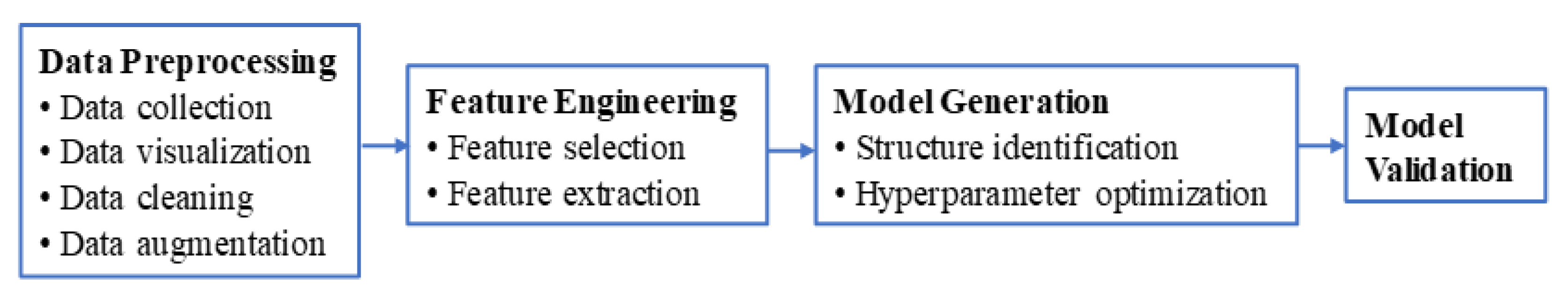
3. The Proposed Pipeline

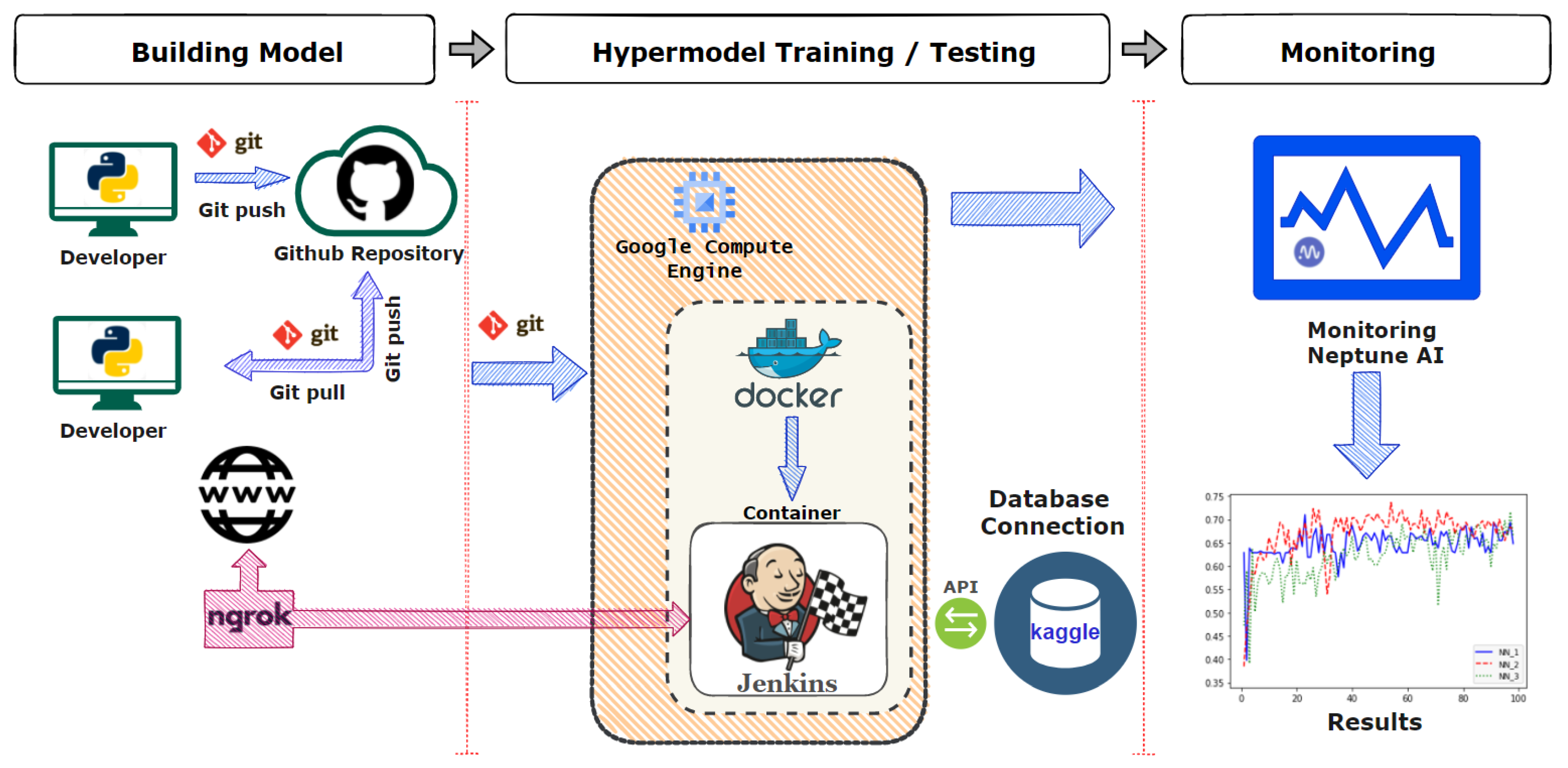
3.1. The Overall Operational Structure of the Pipeline

The ML model that runs on the pipeline is a multilayer perceptron (MLP) that combines layers with typical activation functions (e.g., Relu, Tanh, etc.) and layers with activation functions represented as Hermite polynomials. The use of polynomial activation functions was motivated by the research reported in [42,43], while the problem under consideration is to perform classification tasks. The key point is to use the benefits of the AutoML workflow and perform hyperparameter optimization in terms of Bayesian optimization. The ultimate research target is to determine whether the presence of layers with polynomial activation functions improves the classification accuracy or not.
The basic structure of the proposed pipeline encompasses three developing stages and is illustrated in Figure 2.
The first stage refers to the building process of the ML model. The source code that is being derived by the development team in the whole software cycle is tracked by the popular Git version control system [44]. The main benefit provided by this stage is the ability to construct and test any ML model configuration without considering intermediary processes (such as the download and preparation of the dataset) that are traditionally performed manually in ML model generation. Moreover, a master branch is created that contains the final code and some custom branches, where each one of the developers work on to test the derived code before merging it with the master branch. To this end, the cooperation between different developers is accelerated, since the information is available online and updated in a dynamic manner, as opposed to using static methods, such as shared files.
In the second stage, cutting edge technologies are used to appropriately handle the information flow. This stage performs the execution of the “runner.py” file, which includes all the appropriate dependencies needed to allow the file to be correctly compiled and, then, run the above-mentioned ML process. The main executing computer machine is a virtual machine (VM) provided by Google, the characteristics of which are presented in Section 3.2.3. On the VM, the Docker software [45] is installed, and a Jenkins Docker container [46] is created, which plays the role of the server that will handle the whole process between developing and monitoring. The above containerization technology provides flexibility in managing the Jenkins dependencies errors that may occur during the various installations, which might not affect the VM itself. In this stage, Jenkins pull the source code from Github that developers pushed. After checking all the appropriate functionalities, such as the python version of the environment, Jenkins sends an execution request to the physical processors of the VM. Additionally, Jenkins creates a job folder on the VM, where all the files of the specific Jenkins job will be stored. At this point, it is emphasized that the Jenkins server creates various jobs that can be executed in parallel (if the physical resource system allows it). Moreover, Jenkins jobs can pull the source code from any working branch, giving the ability to test ideas that are not approved, and which are yet to be merged into the master branch, i.e., in the final ML product. In our application, the above-mentioned execution is carried out in terms of the following steps: (a) connecting with the Kaggle database, using the Kaggle API [47], (b) data preprocessing, (c) hyperparameter optimization using Bayesian optimization, (d) training and evaluation of the resulting ML models, and (e) sending monitoring requests to the Neptune AI platform [48] (see the next stage below). It is strongly pointed out that the use of the docker containerization technology is a crucial MLOps practice, as it provides a degree of isolation that prevents conflicts between the various components of a ML pipeline. Traditionally, the whole process would run in an executable computer program, and if anything goes wrong, technicians will have to repair the entire system. The usage of Docker simply terminates the docker container and begins a new one, saving further time. Moreover, Docker makes it simple to scale applications by running several instances of a container, enabling the deployment of ML models across numerous servers.
The third part of the pipeline contains the model’s monitoring process, which is carried out by the Neptune AI platform. The monitoring process is also a crucial MLOps practice, performed efficiently by the Neptune AI software. The main advantage provided by the Neptune AI is the ability to effectively connect with Python codes by using specialized callback functions that track specific metrics (such as validation accuracy) during the training and evaluation procedures. In addition, monitoring allows for tracking the performance of the model over time, and it is in the position to record the exact time instant when the model’s degradation starts to occur. This can be very helpful in identifying problems early and taking action to improve performance.

3.2. Technologies Used in the Pipeline

In this section, the exact operation of each one of the technologies used in the pipeline is analytically presented, including a reference to the Bayesian optimization that performs the hyperparameter tuning process.

3.2.1. Git Version Control System

Git is a widely popular distributed version control system [44]. Its main task is to manage/track changes, existing in a source code. It gives the capacity to the developers in collaborating during the code creation and moreover to revert to any previous code version if it is necessary [49]. Git has proven to be very effective in handling large projects, supporting many contributors. The efficiency and productivity of software developers can be improved via Git, allowing them to collaborate more effectively, and providing them a clear record of code changes [49,50].
In this paper, the Git version control system is employed to track and manage code changes in the resulting Python source codes. In addition, the proposed pipeline uses it to revert the information flow to prior versions. This is especially handy when, on several occasions, it is needed to return to a previous version of the model, as the current version does not perform efficiently. Finally, the source code created in the model’s building stage is stored in the Github repository, and it is pushed via the Git version control system.

3.2.2. Jenkins Automation Server

Jenkins constitutes an open-source automation server that allows for automated building, testing, and deploying of produced software [46]. Its source code is written in Java and offers several plugins, obtaining high-level support as far as the design of several types of software is concerned, such as web-based, mobile, and cloud-based applications. Its capability in providing full automation during the progress of software design and implementation reflects on significantly lowering the needed time and effort [51,52]. A key point that makes Jenkins very useful is its compatibility with many tools and technologies, such as version control systems, testing frameworks, and deployment tools. As a result, it can be used as a single control point in the entire software creation, spanning from source code to applications [46].
In the current contribution, the Jenkins server constitutes the heart of the proposed pipeline. Its main role is to organize information that exists in repositories, connect separate technologies, and execute the appropriate tasks. Moreover, it is used to construct Jenkins jobs, running within the pipeline.
In more details, the main target of using the Jenkins automation server is to establish and handle the connection between the source code created in the building model stage (stored in Github repository and pushed via the Git version control system), the execution of the target file (i.e., the runner.py), and the connection with the monitoring system Neptune AI. To accomplish the above target, a Jenkins job, inside the web interface, is properly configured in order to be responsible for the whole process.
In this job, important pipeline parameters are defined, such as (a) the Github repository that has to be connected with and pull the source code from it, (b) the appropriate security level of this connection, (c) the Git branch to look in, and (d) the Jenkins script file that contains configuration information about the pipeline steps and the automated built triggers after Git commit events that enable the option of the job to run automatically after commits (we used the option Github hook trigger for GITScm polling as our main source code in Github).

3.2.3. Google Cloud Virtual Machines

Google Cloud Virtual Machines (VMs) are cloud-based computing resources that allow users to run applications and workloads on virtual servers. They are part of the Google Cloud Platform (GCP), which is a cloud computing platform that offers a range of computing, networking, storage, and other services.
Google Cloud VMs provide flexible, scalable, and reliable computing resources on demand, allowing users to easily configure VMs, meeting the specified requirements of the corresponding applications and workloads. They also offer a wide range of features and options, such as the ability to select from a variety of operating systems, processor types, and memory sizes, as well as the ability to customize the networking and security settings of the VMs [53]. Table 1 depicts the properties of the Google Cloud VM, used by the proposed pipeline.

3.2.4. Ngrok API

Ngrok is a reverse proxy tool, allowing for the exposure of a local server, public to the internet. Usually, it is used for testing web applications, running on a local machine or shared local environment. One of the main advantages of Ngrok is its simplicity and ease of usage. It requires minimal setup, and it is compatible with a variety of programming languages and frameworks. Ngrok also offers several useful features, such as its ability to inspect traffic and provide secure tunnels, which are helpful in debugging and testing [54].
In the proposed pipeline, Ngrok API is used to expose the Jenkins local web server to the internet. This choice provided the ability to harmonically collaborate among the members of the team and to access the Jenkins jobs through a secure public Ngrok web address, without having to deploy it to a shared network or cloud environment.

3.2.5. Kaggle API

The Kaggle API is a set of tools designed for interacting with the Kaggle platform from the command line. It allows the managing of the user’s Kaggle account and enables both the download and the upload of datasets [47,55].
In the current framework, the efficient usage of Kaggle API is based on installing the Kaggle Python package, along with corresponding user authentication. Once authenticated, the API is employed to perform a list of appropriate actions, such as the data sets’ download. In addition, the Kaggle API provides a convenient way to interact with Kaggle database resources and services directly from the Python source code. The above configuration empowers the automation of data retrieval (i.e., download) directly from the Kaggle database into the pipeline, without having to manually download the data.

3.2.6. Docker Platform

Docker is a containerization technology that enables developers to bundle applications and dependencies into lightweight, portable containers that may be launched on any machine [56]. It has the capacity to assist in the creation, testing, and deployment of consistent and dependable software applications [57]. As such, it allows the construction and testing of programs on their own systems, using the same tools and dependencies that are used in production, reducing the risks arising in different environments [56,58]. In addition, there exist certain security benefits associated with the usage of Docker. For example, containers can operate in an isolated environment, without sharing the host operating system’s kernel, making them less susceptible to security vulnerabilities. In this direction, the employment of Docker can reduce the attack surface of applications, as containers only include the necessary libraries and dependencies required for their operation [58,59].
In the proposed pipeline, the Docker containerization technology assists the software provisioning, i.e., the process of installing, configuring, and setting up software applications for end-users inside an executor. As such, it is used to construct a Jenkins container, as described in Section 3.2.2. The main benefit, arising from that choice, is that the software provisioning, as far as the python libraries (i.e., Tensorflow, Keras, etc.) are concerned, becomes independent from the local Google VM engine system, thus not affecting the local system if something goes wrong in the provisioning step. Based on this MLOP practice, it is feasible to save computational time by just destroying the Jenkins container instead of applying a workaround debugging process, which is time consuming.

3.2.7. Monitoring through Neptune AI

Neptune AI is an open-source machine learning and data science platform that allows researchers to track and share their work easily [48]. Through Neptune ML, metadata can be organized in a single accessible place. In a nutshell, it provides the subsequent features that are useful for building ML models [48]:
  • Easy integration with popular libraries and tools (e.g., TensorFlow, Keras, PyTorch, Scikit-Learn, etc.)
  • A web-based interface for tracking and organizing experiments and projects
  • Collaboration features that allow multiple people to work on the same project
  • A platform for sharing and reproducing results
  • Flexibility in handling complex projects that deal with different experiments and the proper data/results tracking
In the proposed pipeline, the Neptune AI platform constitutes the monitoring system, which is an MLOps process. To accomplish this task, the pipeline employs Python callback functions to track certain metrics, such as validation accuracy. These kinds of metrics are available by the Neptune AI and can be easily integrated and combined with Tensorflow. Finally, inside its web interface, the pipeline uses the comparison capabilities between different simulations, offered by Neptune AI.

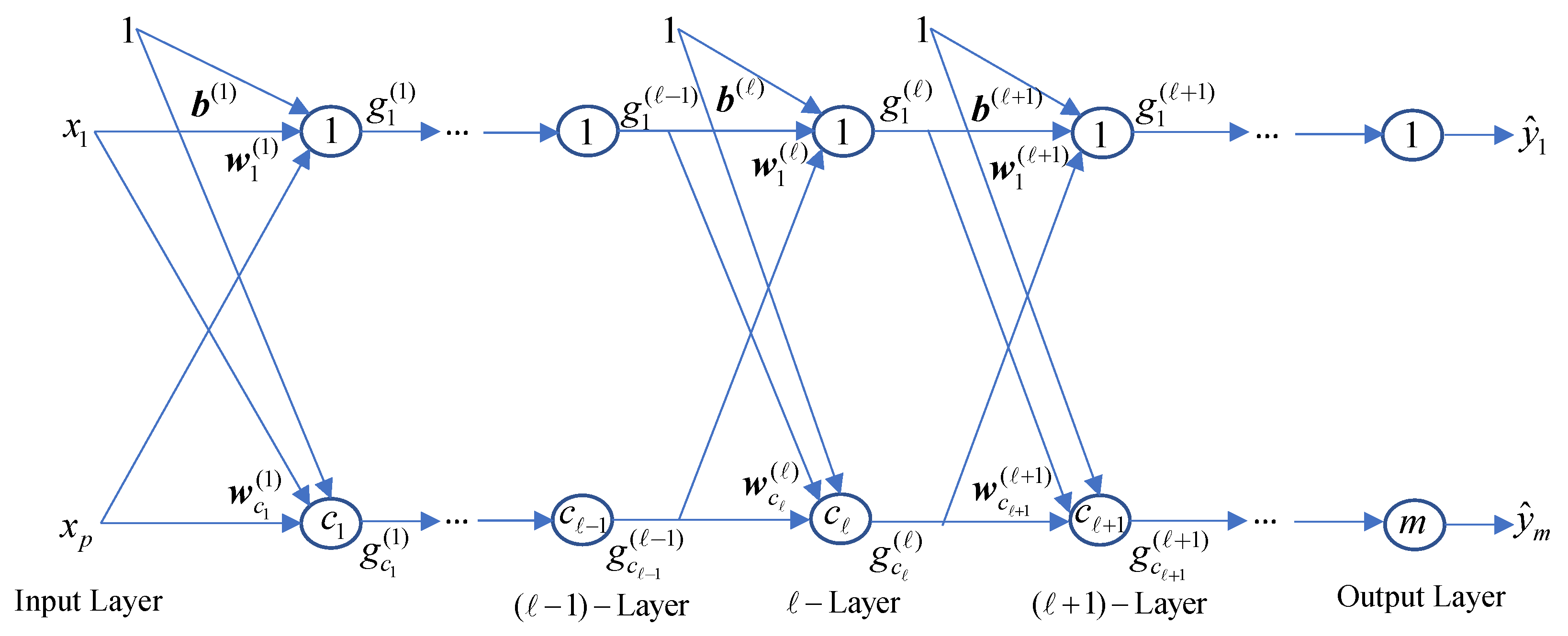
3.2.8. Polynomial Neural Network

The neural network used in this paper is a multi-layer perceptron (MLP) with several layers. Each layer can be a typical layer, with standard activation functions, such as the Relu or the Tanh, or a layer with activation functions, such as Hermite polynomials [42,43]. The Hermite polynomials, with order n, are generated by the next differential equation,
H n ( z ) = ( 1 ) n e z 2 d n dz n e z 2
where z R . They are orthogonal under the next condition.
+ H n ( z )   H m ( z )   e z 2 d z = 2 n n ! π   δ n m  
where δ n m is the Kronecker delta. An easy way to obtain the Hermite polynomials is the following recursion relation,
H n ( z ) = 2   z   H n 1 ( z ) 2   ( n 1 )   H n 2 ( z )
with the initial conditions being as follows: H 0 ( z ) = 1 and H 1 ( z ) = 2 z . The reason for choosing Hermite polynomials is that, according to Equation (2), they are orthogonal with respect to the whole set of real numbers, whereas other polynomials retain their orthogonality over the interval [–1, 1], only.
In the MLP network under consideration, the nodes of each layer have the same activation functions, while different layers may have different activation functions. Thus, there exist many architectures, each of which uses a specific sequence of layers with different activation functions. Figure 3 illustrates a possible network’s structure.
In this figure, the network admits an input data vector x = [ x 1 ,   x 2 ,   ,   x p ] R p , and it includes L hidden layers, where three hidden layers in sequence are clearly shown, i.e., the ( 1 ) -Layer, the -Layer, and the ( + 1 ) -Layer, with = 1 ,   2 ,   ,   L . To study the network’s functionality, it is assumed that the first of the above three layers includes c 1 with ReLU activation functions, the second includes c nodes with n-order Hermite polynomial activation function, while the third one includes c + 1 nodes with Tanh activation functions. Thus, the outputs of these layers read as follows,
g i ( 1 ) ( z ) = ReLU ( z ) ,           i = 1 ,   2 ,   ,   c 1
g j ( ) ( z ) = H n ( z ) ,           j = 1 ,   2 ,   ,   c
g k ( + 1 ) ( z ) = Tan h ( z ) ,           k = 1 ,   2 ,   ,   c + 1
The weight and bias matrices of the -Layer are, respectively, written as,
b ( ) = [ b 1 ( ) ,   b 2 ( ) ,   ,   b c ( ) ] T
W ( ) = [ w 1 ( ) T ,   w 2 ( ) T ,   ,   w c ( ) T ] T
where,
w j ( ) = [ w j , 1 ( ) ,   w j , 2 ( ) ,   ,   w j , c 1 ( ) ] T ,         j = 1 ,   2 ,   ,   c
To this end, the output of the -Layer is g ( ) :   R c 1 R c and is calculated as,
g ( ) ( x ) = [ g 1 ( ) ( x ) ,   g 2 ( ) ( x ) ,   ,   g c ( ) ( x ) ] T
with
g j ( ) ( x ) = g j ( ) ( w j ( ) T g ( 1 ) ( x ) + b j ( ) )
Note that, in Equations (4)–(6), the variable z is: z = w j ( ) T g ( 1 ) ( x ) + b j ( )     R .
The above analysis for the -Layer is similarly applied to the rest of the layers, considering the respective activation functions, as reported in Equations (4)–(6).

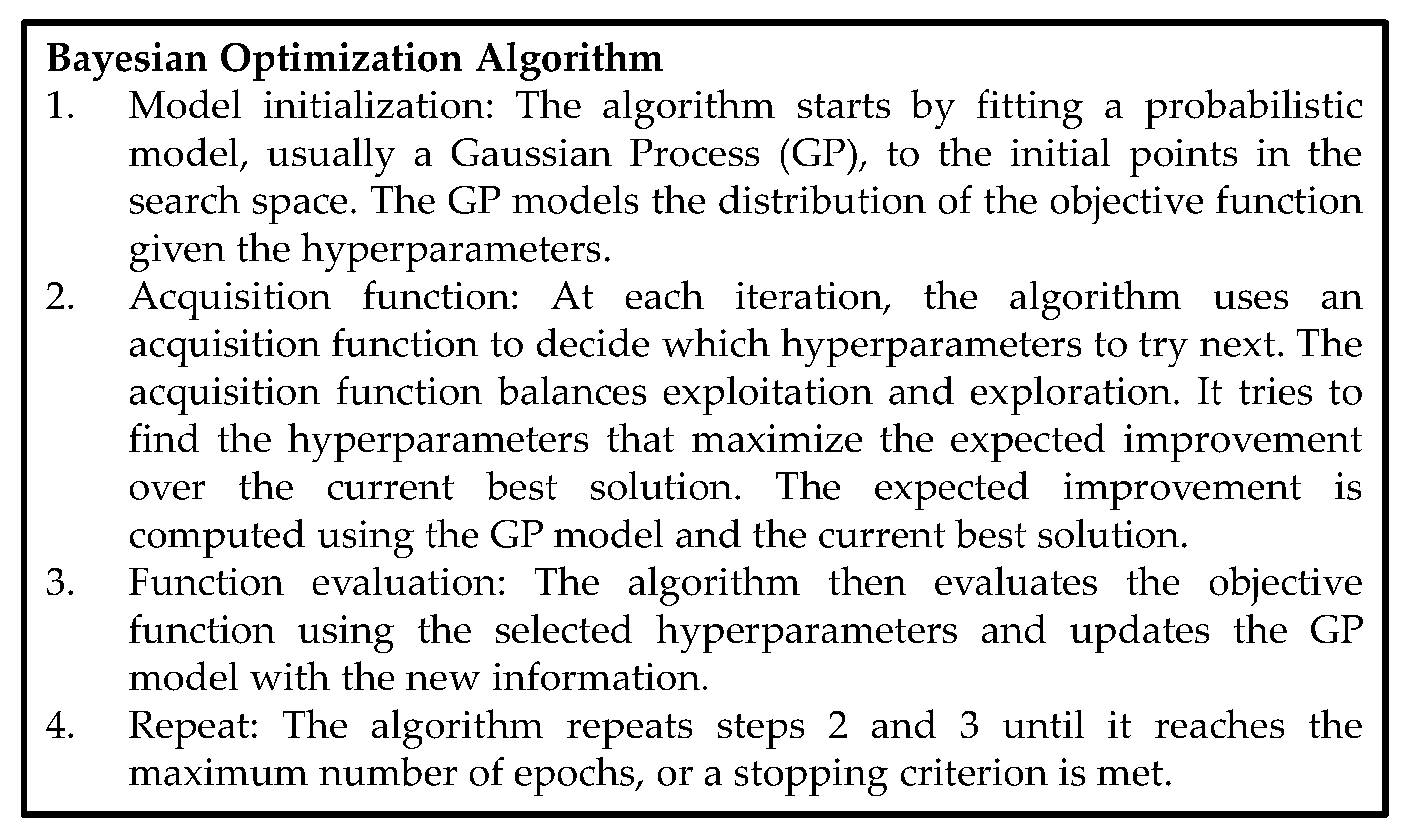
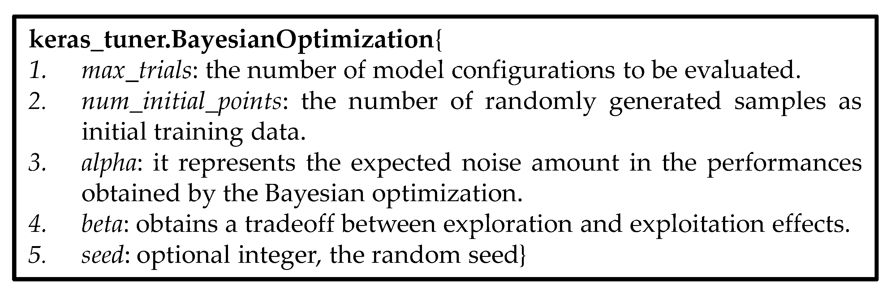
3.2.9. Hyperparameter Tuning

Hyperparameter optimization concentrates on calculating optimal values for the set of ML model’s hyperparameters, which obtain the best model’s classification performance evaluated on the testing data set [60]. For example, in the case of a neural network, the hyperparameters can be the number of layers, the learning rate, the batch size, etc. Traditionally, the hyperparameters have been decided by the model’s designer before the training process, while the model’s parameters have been calculated through the training process. However, this strategy has imposed certain difficulties as far as the reproducibility and reusability of the models are concerned [10,41,60]. Another difficulty reflects on the fact that different datasets require different sets of hyperparameters. As such, the usage of manual intervention in deciding an appropriate set of hyperparameters for a ML model appears to be a complex task, which, in most of the cases, is not solved optimally [26,40,60].
The mathematical formulation of the hyperparameter tuning used in the current contribution is described by the subsequent analysis.
Let S denote the available data set, and I symbolizes the ML algorithm chosen to perform the modeling process, e.g., the Adam optimizer [61]. The set of hyperparameters involved in the above modeling process is described as a = [ a 1 ,   a 2 ,   ,   a m ] . Thus, the number of hyperparameters is equal to m. The domain of values for the ith hyperparameter is denoted as A i , yielding a search space, written as
A = A 1 A 2     A m = i = 1 m A i
where stands for the product space operator. Thus, for the hyperparameter vector, the following holds— a   A . The data set S is divided into two disjoint sets, namely, the training data set, S t r a i n , and the testing data set, S t e s t , where the former is used to train the model, while the latter is used to evaluate its performance. Substituting a set of hyperparameter values, a, in algorithm, I, is symbolized as I a , and the result is the generation of a model to describe the dataset, S. To this end, the objective function to be optimized reads as follows [60]:
a o p t = arg min a A E ( S t r a i n ,   S t e s t ) S ( L ,   I a ,   S t r a i n ,   S t e s t )
where L is the user-defined classification loss function, obtained by implementing the algorithm I a on the training set S t r a i n , and E stands for the expected value. Popular approaches to quantify the function, , are the holdout and the cross-validation error for a given user-defined loss function [60]. On the other hand, the optimization of the function, , is usually carried out by specialized hyperparameter optimizers, such as the Grid search method [60,62], the random search approach [60,63], the Bayesian optimization algorithm [60,64,65], etc.
In this paper, the types of hyperparameters taken into account are,
  • the learning rate parameter
  • the number of layers
  • the number of nodes in each layer
  • the type of activation function in each layer (the activation function types are given in Equations (4)–(6))
The domains of values that define the search space for the above hyperparameters are given in Section 4.
In addition, in the current study, the loss function L is the cross-entropy objective function, the algorithm I a , to minimize the function, L, is the Adam optimizer [61]. The hyperparameter objective function, , is the validity accuracy, quantified by the rate of the correct classified instances, while the hyperparameter optimizer is the Bayesian optimization algorithm.
In view of Equation (13), the basic information flow in the hyperparameter tuning framework used in this paper is as follows. The initialization of the hyperparameter optimizer provides a set of hyperparameter values a to the classifier, and the algorithm I a employs those values to minimize the loss-function, L, using the training data set, S t r a i n . Then, the loss-function, L, is evaluated on the testing data, S t e s t , and the resulting loss-function values are fed back to the hyperparameter optimizer, which uses them to spotlight areas in the search space that include promising hyperparameter values that optimize the function . To this end, these hyperparameter values, a , are provided to the algorithm I a , and the above approach continues until convergence. It is emphasized that, while the model’s parameters are optimized in terms of the training data set S t r a i n , the hyperparameters are estimated in terms of the values of the loss-function L, evaluated on the testing data set, S t e s t . Therefore, the testing data are not used (i.e., as training data) by the Bayesian optimizer, and, rather, their corresponding evaluated loss-function values are employed to guide the selection of new hyperparameter values.
The problem with hyperparameter optimization is that minimizing the hyperparameter’s objective function in Equation (13) is computationally intensive [40,60]. Each time, different hyperparameters are used, and the model’s training and evaluation processes are to be repeated. As mentioned above, to address that issue, various optimization approaches have been applied, such as grid search [62], random search [63], and Bayesian optimization [64,65].
Grid search [60,62] checks all the possible combinations of the hyperparameters and, therefore, it is subjected to the problem known as the “curse of dimensionality problem”, which directly implies that the whole procedure is very computationally complex.
An alternative to grid search is the random search [60,62], which tests random samples in the hyperparameter search space, thus alleviating the intensive computational cost of grid search.
Finally, the Bayesian optimization algorithm [60,64,65] treats the objective functions as a sample taken from a Gaussian process over the hyperparameter search space. The resulting posterior probability gives information about the possible function’s global optimal position. After the probabilistic model is generated, the algorithm utilizes an acquisition function and searches the space by obtaining a tradeoff between exploration and exploitation. Exploitation guides the search to nearby points, where the performance is likely to increase, while exploration searches a different area of the search space, where another local (or even the global) minimum exists. The choice of acquisition function is crucial for the performance of the algorithm. The most used acquisition function is the expected improvement [64,65]. Other options include the probability of improvement, the lower confidence bound, and the upper confidence bound [60,64]. Figure 4 depicts the basic steps of the Bayesian optimization algorithm.
The Bayesian optimizer provides several advantages when applied to hyperparameter tuning. For convenience reasons, some of them are enumerated, as follows: (a) it incorporates prior knowledge about the hyperparameters to assist the search, such as domain-specific knowledge or the results of previous runs, (b) it is able to handle constraints imposed on the hyperparameters, such as bounds on their values, etc., (c) taking the advantage of the probabilistic model, it provides an efficient exploration of the search space, and (d) it can effectively cope with noisy or expensive evaluations by using Gaussian processes to model the uncertainty existing in the evaluations.
To this end, the proposed pipeline uses the Bayesian optimization approach to perform the optimization of the objective function reported in Equation (13). To accomplish that task, the Bayesian optimization tuner from the Keras API is used [66]. The basic arguments of the tuner are depicted in Figure 5. The values of the arguments reported in the above table and used in this paper are reported in Section 4.

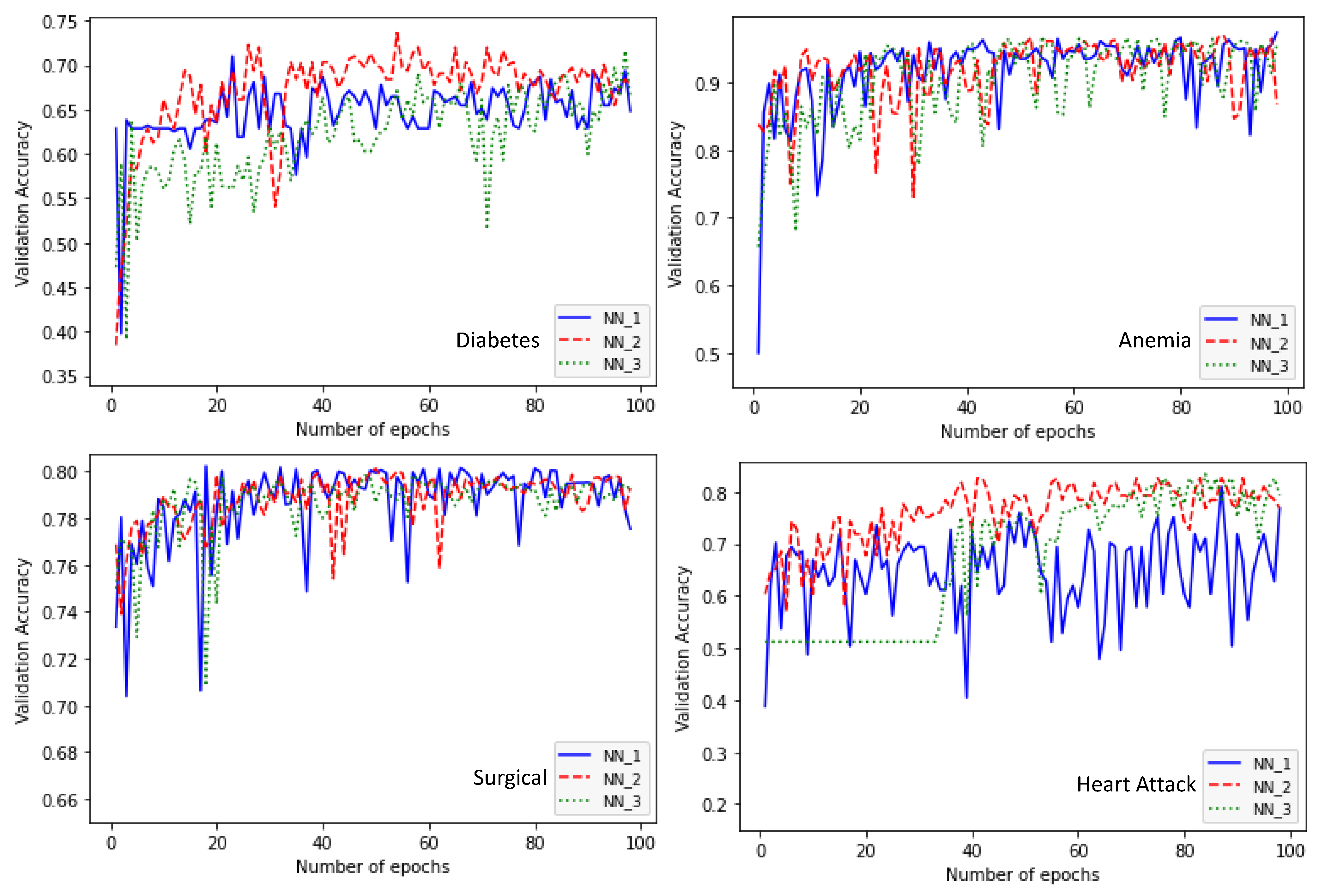
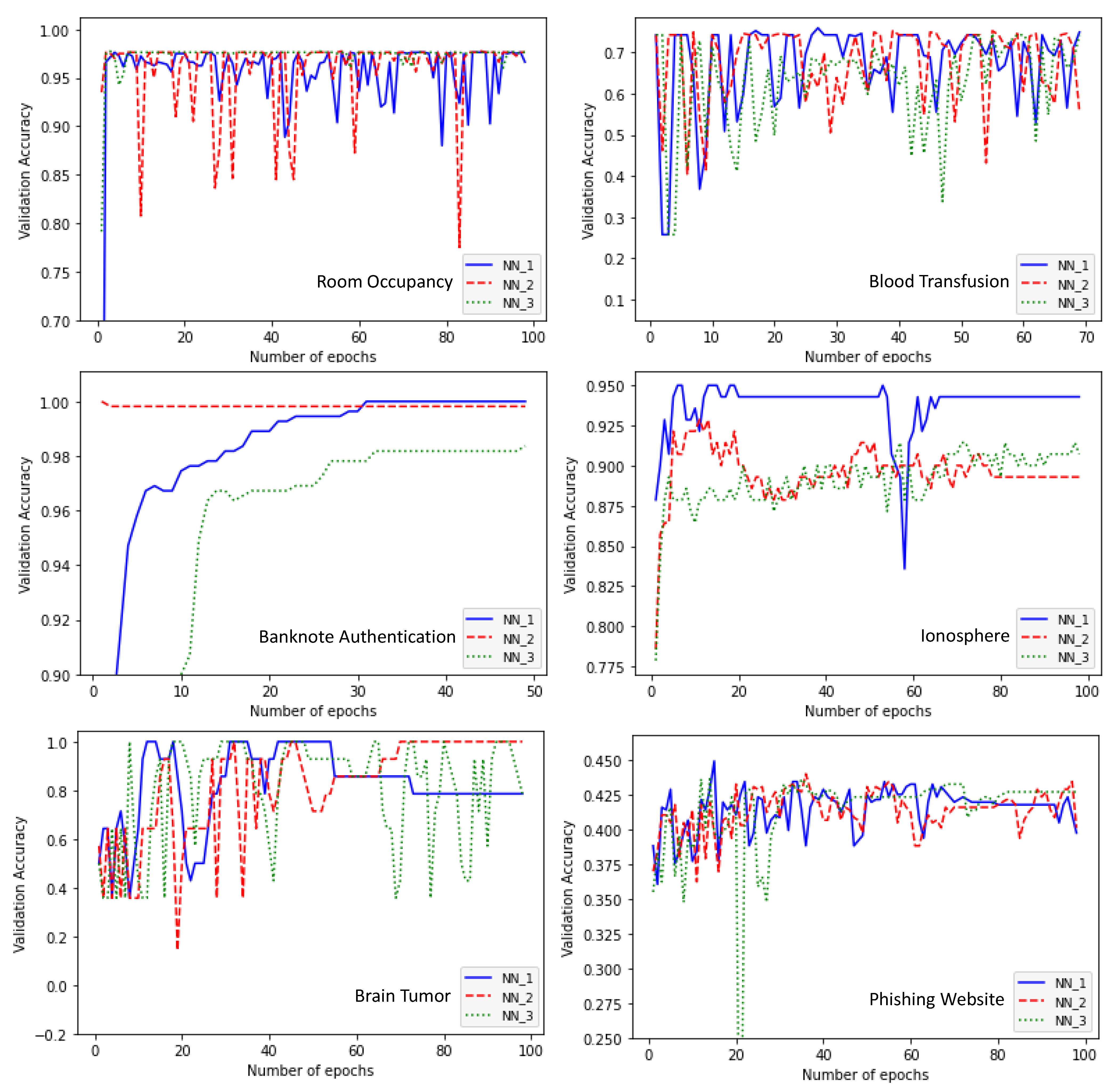
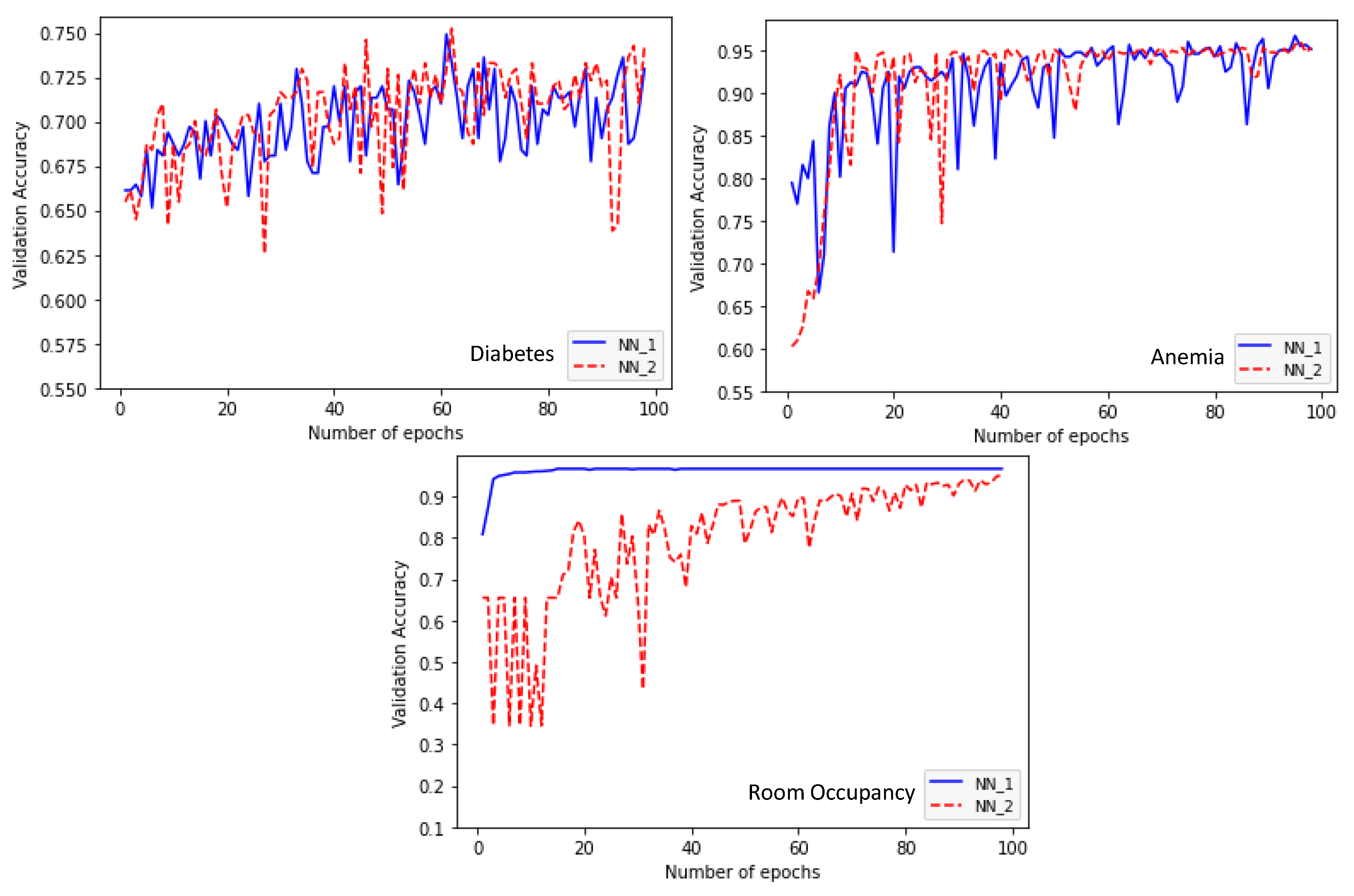
4. Experimental Study

This section presents the results of the simulations that were executed by the proposed AutoML pipeline. Ten data sets were taken from the Kaggle ML database, using the Kaggle API to perform the experiments, the properties of which are shown in Table 2.
As indicated in that table, small datasets were used to perform convenient experimentation using less computational time to run each simulation case. To do so, an extra size restriction of 10 Mb was used in the kaggle.api.dataset_list function, which was responsible for searching for a dataset with a specific predefined criterion. That selection criterion was to refine datasets that include less than 4000 sample instances. As shown in Table 2, nine out of ten datasets fulfill the above criterion, except for the “Surgical” data set, which includes a significantly larger number of instances. The reason behind that choice was the need to test and compare at least one much larger data set in terms of computational time and accuracy, as well. Another interesting case is the “Brain Tumor” data set, which, although it contains a very small number of instance samples, the number of feature variables is very large. Again, the target was to check whether there is a significant impact of the number of input features upon the computational time needed by the pipeline to perform the simulations. At this point, it is strongly emphasized that all data sets concern binary classification tasks.
Table 3 depicts the domains of values for the hyperparameters. All possible combinations between the hyperparameter values reported in that table define the hyperparameter search space. In addition, as shown in Table 3, the polynomial activation functions were taken to be Hermite polynomials of second order, denoted as H2, i.e., in Equations (3) and (5), it was set to n = 2.
Note that Table 3 states that three out of four types of hyperparameters utilize discrete set values as their domains. Therefore, the hyperparameter search space is a hybrid space, combining real and discrete domains. It is especially noted that, for the last hyperparameter in Table 3, three types of activation function were used, as also analyzed in Equations (4)–(6).
The implementation of the Bayesian optimization was carried out in terms of the above hyperparameter search space. For computational complexity reasons, an upper limit of 100 trials was chosen (i.e., the argument max_trials defined in Figure 5), meaning that, for each dataset, at most, 100 models were trained and evaluated, and the validation results were fed into the Bayesian optimization module.
Moreover, random seed was used to enhance the stochastic behavior of the optimizer during different runs. Table 4 presents the values for parametric arguments of the Keras Bayesian optimization tuner, which were defined in Figure 5.
As mentioned previously, the loss function for the Bayesian optimization algorithm was the validation accuracy evaluated on the testing data in terms of the amount of correct classified instances. Relationally, the objective function for the training process of each model was the cross-entropy, which was minimized using the Adam optimizer.
To conduct the experiments, each data set was randomly divided into a training set, containing 60% of the original data, and a testing set, containing the rest of the 40% of the original data. The models’ validation accuracies refer to the evaluations of the models on the testing data.
The main research problem was to check whether the use of second order Hermite polynomial activation functions can improve the accuracy of the MLP network in binary classification tasks.
However, it is crucial to mention that evaluating the polynomial neural network is not the core of our work but only the application through which the functionality of the proposed pipeline is tested and evaluated.
To investigate the above problem, four experiments were conducted.
The first experiment concerned the monitoring of the trained models and selecting the best three MLP neural network (NN) models, namely, NN_1, NN_2, and NN_3. The selection was based on the best three validity accuracy performances on the testing data. The results were derived from the whole machine learning training/testing process and captured automatically by the Neptune AI platform using callbacks functions inside the runner Python file. Table 5, Table 6 and Table 7, and Figure 6 and Figure 7, depict the experimental results obtained by the first experiment.
Based on Table 5, Table 6 and Table 7, the obtained total hyper-tuning time results imply that the implementation of the proposed AutoML pipeline is a fast execution process, given the large number of models (as defined by the max_trials parameter in Table 4) that were generated and evaluated.
Three additional important remarks are as follows: (a) apart from few cases, the best models were obtained when the learning rate is equal to 0.01, (b) apart from the NN_1 in the Banknote Authentication dataset, all models use five layers in total, (c) as far as the total time needed to perform the hyperparameter optimization, the “Surgical” dataset obtained the larger execution time (as it was expected in the first place), while, for the “Brain Tumor” data set, the time is retained within the levels appeared in the rest of the data sets (mainly because the number of instances is very small).
It is noted that 30 MLP neural network models were created, where eight have no Hermite polynomial layers, 10 have one, 10 have two, and two have three Hermite polynomial layers. Thus, 73.3% of the produced best models have Hermite polynomial layers. This fact directly indicates that the behavior of the MLP is increased by using such type of layers.
Finally, the comparative behavior of the three best models, illustrated in Figure 6 and Figure 7, directly support the results depicted in the above tables as far as the validation accuracy is concerned.
The second experiment compares the best model obtained by executing the hyperparameter optimization in the search space given in Table 3, and the best model obtained by using the hyperspace, where the domain of values for the hyperparameter “type of activation function” is: {“ReLU”, “Tanh”} (i.e., the second order polynomial activation function is excluded). The former hyperspace is called “Hyperspace A”, while the latter is called “Hyperspace B”. Thus, the best neural network trained in Hyperspace A includes layers with Hermite polynomial activations and is denoted as NN_1, while the best model trained in Hyperspace B does not contain polynomial layers and is denoted as NN_2.
The purpose of the experiment is to evaluate the needed computational energy to produce models with performance comparable to the performance of the best models relative to the hyperspace that does not contain polynomial in its structure.
To conduct the experiment, five datasets were used, i.e., Diabetes, Anemia, Room Occupancy, Banknote Authentication, and Ionosphere. Table 8 and Table 9, and Figure 8 and Figure 9, illustrate the results of the current experiment.
The last column in Table 8 and Table 9 is the mean hyper-tuning time, which is the mean value of the AutoML pipeline’s execution time for performing the hyperparameter optimization in Hyperspace A and Hyperspace B.
Based on Table 8 and Table 9, the following remarks can be pointed out: (a) the mean execution times, presented in the last columns of those tables, are small, given the large number of models created and tested by the pipeline (as indicated by the parameter max_trials in Table 4); (b) in four out of five datasets, the models with Hermite polynomial activation functions appear to have better classification performance in terms of the validity accuracy; (c) similarly to the first experiment, in most of the cases, the resulting learning rates are equal to 0.01; (d) in the Banknote Authentication dataset, both models include the smallest number of layers (i.e., three layers).
To this end, the models’ behaviors depicted in Figure 8 and Figure 9 support the superiority of the models that include layers with Hermite polynomial activation functions.
Based on the results obtained by the two experimental cases, it is safe to conclude that the proposed AutoML generated and validated a very large number of neural network models, utilizing relatively small execution time. At this point, it has to be emphasized that the heaviest computational task was hyperparameter optimization.
As far as the research question that was used to investigate the pipeline’s performance, it was shown that the use of Hermite polynomial layers is in the position to increase the performance of a typical MLP network.
In the third experiment, each data set was divided into three disjoint subsets, namely, the training, testing, and validation data. The training data were used to optimize the machine learning model’s parameters, and the testing data were used to evaluate the model’s loss function values and use them to assist the hyperparameter optimization, and the validation data were used as independent control data for assessing the resulting machine learning models. Note that, as mentioned in Section 3.2.9, while the training data are directly used in the learning process, the testing data are involved indirectly in the hyper-tuning procedure by providing the estimated loss function values to the Bayesian optimizer. On the other hand, the validation data are not used by the learning mechanism at all, thus giving a reliable means to objectively evaluate the resulting models’ performances.
To provide a proof of concept, two datasets were used, namely, the Diabetes and Anemia data. For each dataset, the validation data consisted of 20% of the original data, while the rest of the 80% of the original data were divided into 75% training data and 25% testing data.
To conduct the experiment, two simulation cases were performed, using the Bayesian optimization parameters depicted in Table 4.
The first simulation case used the hyperparameter search space, shown in Table 3, and it is similar to the first experiment analyzed previously. As such, it concerned the monitoring of the trained models and selecting the best three MLP neural network (NN) models, namely, NN_1, NN_2, and NN_3, evaluated on the validation data.
The second simulation case used the Hyperspace A and Hyperspace B, as described in the second experiment presented previously. More specifically, this simulation case compares the best model obtained by executing the hyperparameter optimization in Hyperspace A, and the best model obtained by using the Hyperspace B. Thus, similarly to the above-mentioned second experiment, the best neural network trained in Hyperspace A comprises Hermite polynomial layers and is symbolized as NN_1, while the best model trained in Hyperspace B does not include polynomial layers and is symbolized as NN_2.
Table 10 and Table 11 show the results obtained by the first and second simulation case, respectively. Note that, in both tables, the classification accuracy is evaluated on the validation data.
In view of Table 10 and Table 11, the following remarks are spotlighted. First, except for one model, the optimal learning rates appear to be equal to 0.01, while, in most of the cases, the number of layers is equal to five (note that the same observations were obtained in the previous experiments, also). Second, for every model reported in Table 10, at least one layer appears to be a Hermite polynomial layer, while, for each dataset, all models obtain similar behaviors as far as the classification accuracy is concerned. In addition, in Table 11, the models with Hermite polynomial activation functions obtain better classification accuracy, which directly implies that performing the hyperparameter optimization in Hyperspace A is more efficient than in Hyperspace B (an observation that was also derived by the second experiment presented previously). Third, the time duration needed to perform the models’ design lies within similar levels for all cases and models, something that was expected given that the complexity of the two datasets is similar.
Finally, the subsequent analysis investigates the effectiveness of the proposed AutoML pipeline in evaluating its performance on the testing data and on validation data, as they were defined above. Since the first simulation case of the current experiment (i.e., the third experiment) is similar to the first experiment and the second simulation case is similar to the second experiment, the results in Table 10 are compared with the results in Table 5, whereas the results in Table 11 are compared with the ones reported in Table 8. The comparison analysis concerns the classification accuracy and the hyper-tuning time duration, regarding the Diabetes and Anemia datasets.
The first comparative remark is that the accuracies obtained by the validation data in Table 10 and Table 11 are slightly inferior to the respective accuracies calculated on the testing data in Table 5 and Table 8. Although this was expected in the first place, the difference is not large, which directly implies that the pipeline appears to have a robust behavior in dealing with unknown data. The second comparative remark concerns the hyper-tuning time. Regarding Table 5 and Table 10, it can be easily seen that the total hyper-tuning time durations are almost equal, while a similar observation is derived by comparing Table 8 and Table 11 as far as the mean hyper-tuning time is concerned. The last remark suggests that the division of a dataset in three parts (i.e., training, testing, and validation data) has not significant impact on the execution time of the pipeline’s simulations.
The last experiment concerns the quantification of the time difference between the manual implementation of several activities involved in the overall procedure and their respective automated implementation by the proposed pipeline. It is strongly pointed out that this time difference is translated as the time saved by the usage of the proposed AutoML system.
In total, nine processes have been identified as nominates to be applied by manual procedures. These processes are spanned over the three stages of the proposed AutoML pipeline. To provide a convenient presentation of the calculation of the respective time difference for each one of those processes, we proceed with the subsequent analysis.
Regarding the first stage (i.e., the model building stage), the main process that can be manually executed is the continuous Python code generation through the team’s members coordination and collaboration. Note that this process is independent of a specific dataset.
In our pipeline, the collaboration between the team’s members (i.e., developers) is carried out by the installation and operation of the Git version control system. This system is connected with the on-line Github repository, which assists the coordination and collaboration between the team members with the ultimate purpose of the speed up of the model building process, thus resulting in a fully automated collaboration.
In the manual mode, the coordination/collaboration between developers depends on the way they decide to collaborate (by not using the AutoML pipeline), employing different ways to perform the collaboration, such as web-based call meetings.
To investigate the time saved using the Git system in our AutoML framework, a hypothetical case study scenario consistent with the proposed pipeline is studied, according to which it is assumed that there are four developers (and, therefore, four computer machines), and the software has to be released in 30 days. To meet the schedule, the developers make progress every day on the existing code by discussing the needed changes for approximately 30 min/day via web-based meeting. Thus, the time required for the above task is equal to 900 min/month. If the team has decided to share the work/code via cloud repositories (e.g., google drive), it is assumed that the upload and download time (which depends on the connection and the size of the files) is approximately 5 min/day for the four members, resulting in 150 min/month. Finally, taking into account that the coordination may not be perfect, 2 h/month are needed (for the four-member team) to correct the misunderstandings and errors. Thus, without the use of the Git system, the extra time needed to perform the model building process is approximately equal to 900 + 150 + 2 = 1152 min/month.
Considering that, in order to install the Git system in one computer machine, approximately 3 min are required, and since there are four computer machines, the time needed to install the Git system is more or less 12 min. This time must be subtracted from the above estimated time. Therefore, the time saved by using the Git system is approximately 1140 min/month, which means approximately 40 min daily.
Finally, one operation that causes significant time consumption is restoring the code to its previous state. With the use of Git system, that process takes only a few milliseconds, while, without Git, it may take several hours. The evaluation of the time needed in the latter case cannot be quantified, since several factors that depend on the team are involved. In any case, it is safe to assume that the time saved by the Git system is significantly much larger than 40 min/day.
Regarding the second stage (i.e., the hypermodel training and testing stage), the following five processes were executed manually, and the time differences in relation to their automated execution by the proposed AutoML pipeline were measured.
The first process concerns the execution to open the appropriate software (Python IDE) and trigger the build button, the duration of which was approximately 30 s for the first time and approximately 5 s for every next try. Thus, for 100 executions, we obtained 25 + 99 × 5 = 619 s, or approximately 9 min.
The second process concerns the connection with the Kaggle database to search for a specific classification dataset and to download it. The duration of that task depends only on the file’s size and the download speed. In view of this, the advantage provided by the proposed AutoML system is that the search is not performed by opening a browser, but, rather, by inserting keywords into the Kaggle API, using an appropriate Python function provided by the API. In our case, the sizes of all targeted datasets were under 10 MB. The measured mean time difference between performing the process manually and using the proposed pipeline was approximately equal to 6 min for each data set. Given that there were 10 datasets, the overall time saved by employing the proposed pipeline was approximately equal to 60 min.
The third process concerns the creation of a working folder for each dataset and the respective subfolders (i.e., one subfolder for each execution). The difference in time between performing the above task manually and using the proposed pipeline was equal to approximately 3 min/dataset (i.e., including 10 runs for each data set). Since there are 10 data sets, the overall time difference is estimated at around 30 min.
The fourth process concerns hyperparameter optimization. As this process runs inside the Python engine whenever the python_runner.py file is executed, there is no time difference between its manual execution and its execution through the proposed AutoML system.
Finally, regarding the prosed pipeline, to pre-configure a Jenkins job, approximately 10 min were needed. The created Jenkins job was executed automatically (using Web hooks) when a Git commit occurs. Since this job is reusable, it is irrelevant how many times the model is executed, and the above time interval must be subtracted only once from the overall time.
To this end, regarding the 10 data sets, the overall time difference between executing the above processes manually and using the proposed system is approximately quantified as: 9 + 60 + 30 + 0 − 10 = 89 min, which results in approximately 9 min/dataset.
In addition, an extra effort concerns the execution of parallel runs used to create more than one Jenkins jobs to test different code versions. The time needed for this task is difficult to evaluate, but, in any case, it is added to the final total time estimation. This fact directly implies that the time saved by the implementation of the proposed pipeline is greater than 89 min (or 9 min/dataset).
Regarding the third stage (i.e., the monitoring stage), the time difference between its manual implementation and its implementation using the proposed pipeline appears to have a high level of abstraction and mainly concerns the monitoring part of the classification accuracy validation process.
Using our AutoML system, the results produced by the validation process are automatically sent to the Neptune AI platform for making graphs of the loss function, the validation accuracy, the accuracy in the training data, and each metric to be monitored. In the Neptune platform, graphs are automatically produced, enabling the comparison between graphs coming from different runs.
The quantification of the time difference between the manual and the AutoML approaches is described next.
Data that need to be tracked must be saved in files and then read again to produce the desired figures. In our case, each model runs for 100 epochs, and the monitoring process focused on validating the classification accuracy for each one of the above epochs. For each data set, the measured time difference to save the data in a file, to open manually another script that reads these data, and to produce the graphs, was equal to 2 min/(run*dataset). Considering that each data set was manually run 10 times, the resulting time difference was equal to 20 min/dataset (i.e., 200 min in total).
Additionally, there is extra time if someone wants to track another variable, such as the loss function, a procedure that is carried out automatically by the proposed pipeline. The time difference for this procedure was measured as 5 min/dataset (i.e., 50 min in total).
Finally, in the manual implementation, the resulting figures must be uploaded on a shared point (e.g., Google Drive). The resulting time difference to perform that task was estimated to be approximately equal to 3 min/(run*dataset). Since each data set was executed for 10 times, we obtain 30 min/dataset (i.e., 300 min in total).
To summarize, the overall time difference between executing the monitoring stage manually and using the proposed system is approximately equal to 20 + 5 + 30 = 55 min/dataset. Since there are 10 data sets, the overall time difference was equal to 550 min.
Table 12 summarizes all the time differences quantified above.
Note that the time saved by the proposed pipeline in the first process (i.e., the collaboration between the members of the team) is not projected on each data set because it refers to code generation of the whole pipeline and, thus, it concerns all data sets and the possible applications. For the rest of the processes, the above time can be calculated per data set (see last column of the table).
Based on the analysis so far and the results reported in Table 10, it becomes evident that the time saved by the proposed AutoML pipeline is significant, given both the small sized datasets and the simplicity of the MLP networks’ structure. To this end, the time difference is expected to substantially increase for big data sets and more complicated network structures, such as deep learning models.

5. Conclusions

In this paper, an AutoML pipeline to handle the generation and evaluation of ML models was developed. The main task was to use the pipeline in performing architecture and hyperparameter optimization. The pipeline’s implementation obtained fast model creation process, while it was easily repeatable for various datasets and, at the same time, gave the opportunity for a synchronous and efficient collaboration among the members of our team through the Git and Jenkins technologies.
The main steps synthesizing the pipeline’s structure involved the Git source code pulling, auto-triggering of Jenkin’s job, download and preprocessing of the dataset, hyperparameter optimization, and model testing/evaluation tasks. Technologies, such as Git, Jenkins, and Docker, which are widely used in the CI/CD software development, have been used to put in place the aforementioned steps.
The ML model under consideration was a MLP neural network, which included layers with different types of activation functions. More specifically, three types were employed, namely, ReLU, Tanh, and second order Hermite polynomials. The case scenario was to check whether the presence of polynomial layers can improve the performance of the network in classification tasks or not. To test the case scenario, several data sets were taken from the Kaggle ML data base using the Kaggle API. The data sets were used to generate a very large number of ML models, which were tested and evaluated accordingly. The corresponding hyperparameter tuning was carried out in terms of Bayesian optimization. As a result, the performance of the pipeline was evaluated in terms of the computational time.
The general outcomes of the experimental study are summarized as follows: (a) given the large number of models that were generated, the computational time needed by the pipeline to perform the corresponding optimization was small; (b) the presence of polynomial activation functions is in the position to enhance the performance of MLPs in most of the data sets used; (c) the pipeline shows an effective behavior in dealing with data that are not involved (i.e., previously unknown data) in the overall learning process
A very important experimental outcome concerned the quantification of the time difference between the manual implementation of several activities involved in the overall procedure and their respective automated implementation under the umbrella of the proposed pipeline. This time difference is translated as the time saved by the usage of the proposed AutoML system. The results showed that this difference is significant, while it is expected to substantially increase when bigger data sets and more complex machine learning models, such as deep learning models, are to be considered.
At this point, it is strongly emphasized that the current attempt mainly focused on creating an appropriate AutoML pipeline for the automatic development of machine learning models. As such, typical model structures, such as the MLP model, were taken into account. In this direction, the use of deep learning models appears to be very appealing case for extending the current framework, with the ultimate purpose its testing and evaluation in handling more sophisticated machine learning approaches and more complex data sets. As far as the future work is concerned, extensive additional pipeline configurations will be considered in the following directions: (a) to expand the hyperparameter space, (b) to increase the total number of scenario trials, (c) to select alternative hyperparameter optimization methods and libraries, (d) to include additional MLOps practices as far the testing and deployment steps are considered, and (e) to extend the current framework to automatically generate deep learning models.

Author Contributions

Conceptualization, K.F., G.A. and G.E.T.; methodology, K.F., G.A., G.A.P. and G.E.T.; software, K.F. and G.A.; validation, G.A. and G.A.P.; formal analysis, K.F. and G.A.P.; investigation, K.F. and G.E.T.; supervision, G.E.T. All authors contributed to writing the final version of the paper. All authors have read and agreed to the published version of the manuscript.

Funding

This research received no external funding.

Data Availability Statement

Not applicable.

Acknowledgments

The authors thank the anonymous reviewers for their effort to provide very helpful comments that improved the paper.

Conflicts of Interest

The authors declare no conflict of interest.

References

  1. Feurer, M.; Klein, A.; Eggensperger, K.; Springenberg, J.; Blum, M.; Hutter, F. Efficient and robust automated machine learning. In Proceedings of the Annual Conference on Neural Information Processing Systems 2015 (Advances in Neural Information Processing Systems 28), Montreal, QC, Canada, 7–12 December 2015; pp. 2962–2970. [Google Scholar]
  2. Liu, H.; Simonyan, K.; Yang, Y.; Anderson, A.; Zisserman, A. DARTS: Differentiable architecture search. In Proceedings of the 7th International Conference on Learning Representations (ICLR 2019), New Orleans, LA, USA, 6–9 May 2019; pp. 1–13. [Google Scholar]
  3. Zoph, B.; Le, Q.V. Neural architecture search with reinforcement learning. In Proceedings of the 5th International Conference on Learning Representations (ICLR 2016), Toulon, France, 24–26 April 2017; pp. 1–16. [Google Scholar]
  4. He, X.; Zhao, K.; Chu, X. AutoML: A survey of the state-of-the-art. Knowl.-Based Syst. 2021, 212, 106622. [Google Scholar] [CrossRef]
  5. Cheng, S.; Chen, J.; Anastasiou, C.; Angeli, P.; Matar, O.K.; Guo, Y.-K.; Pain, C.C.; Arcucci, R. Generalised latent assimilation in heterogeneous reduced spaces with machine learning surrogate models. J. Sci. Comput. 2023, 94, 11. [Google Scholar] [CrossRef]
  6. Cheng, S.; Prentice, I.C.; Huang, Y.; Jin, Y.; Guo, Y.K.; Arcucci, R. Data-driven surrogate model with latent data assimilation: Application to wildfire forecasting. J. Comput. Phys. 2022, 464, 111302. [Google Scholar] [CrossRef]
  7. Zoller, M.; Huber, M.F. Benchmark and survey of automated machine learning frameworks. arXiv 2019, arXiv:1904.12054. [Google Scholar] [CrossRef]
  8. Karmaker, S.K.; Hassan, M.M.; Smith, M.J.; Xu, L.; Zhai, C.-X.; Veeramachaneni, K. AutoML to date and beyond: Challenges and opportunities. ACM Comput. Surv. 2021, 54, 175. [Google Scholar]
  9. Nagarajah, T.; Poravi, G. A review on automated machine learning (AutoML) systems. In Proceedings of the 5th IEEE International Conference for Convergence in Technology (I2CT), Bombay, India, 29–31 March 2019; pp. 1–6. [Google Scholar]
  10. Kotthoff, L.; Thornton, C.; Hoos, H.H.; Hutter, F.; Leyton-Brown, K. Auto-WEKA 2.0: Automatic model selection and hyperparameter optimization in WEKA. J. Mach. Learn. Res. 2017, 18, 1–5. [Google Scholar]
  11. Autokeras. Available online: https://autokeras.com/ (accessed on 15 October 2022).
  12. Zimmer, L.; Lindauer, M.; Hutter, F. Auto-pytorch tabular: Multiidelity metalearning for efficient and robust autodl. IEEE Trans. Pattern Anal. Mach. Intell. 2020, 43, 3079–3090. [Google Scholar] [CrossRef]
  13. Feurer, M.; Eggensperger, K.; Falkner, S.; Lindauer, M.; Hutter, F. Auto-sklearn 2.0: Hands-free automl via meta-learning. arXiv 2020, arXiv:2007.04074. [Google Scholar]
  14. Khan, M.A.; Iqbal, N.; Imran; Jamil, H.; Kim, D.-H. An optimized ensemble prediction model using AutoML based on soft voting classifier for network intrusion detection. J. Netw. Comput. Appl. 2023, 212, 103560. [Google Scholar] [CrossRef]
  15. Pecnik, L.; Fister, I.; Fister, I., Jr. NiaAML2: An improved AutoML using nature-inspired algorithms. Lect. Notes Comput. Sci. 2021, 12690, 243–252. [Google Scholar]
  16. Ferreira, L.; Pilastri, A.; Martins, C.M.; Pires, P.M.; Cortez, P. A comparison of AutoML tools for machine learning, deep learning and XGBoost. In Proceedings of the 2021 International Joint Conference on Neural Networks (IJCNN’ 21), Shenzhen, China, 18–22 July 2021; pp. 1–8. [Google Scholar]
  17. Renza, D.; Cardenas, E.A.; Jaramillo, C.M.; Weber, S.S.; Martinez, E. Landslide susceptibility model by means of remote sensing images and AutoML. Commun. Comput. Inf. Sci. 2021, 1431, 25–37. [Google Scholar]
  18. Opara, E.; Wimmer, H.; Rebman, C.M., Jr. Auto-ML cyber security data analysis using Google, Azure and IBM Cloud Platforms. In Proceedings of the International Conference on Electrical, Computer and Energy Technologies (ICECET 2022), Prague, Czech Republic, 20–22 July 2022; pp. 1–10. [Google Scholar]
  19. Yan, C.; Zhang, Y.; Zhang, Q.; Yang, Y.; Jiang, X.; Yang, Y.; Wang, B. Privacy-preserving online AutoML for domain-specific face detection. In Proceedings of the 2022 IEEE/CVF Conference on Computer Vision and Pattern Recognition (CVPR), New Orleans, LA, USA, 18–24 June 2022; pp. 4124–4134. [Google Scholar]
  20. Singh, D.; Pant, P.K.; Pant, H.; Dobhal, D.C. Robust automated machine learning (AutoML) system for early stage hepatic disease detection. Lect. Notes Data Eng. Commun. Technol. 2021, 57, 65–76. [Google Scholar]
  21. Mukherjee, S.; Rao, Y.S. Auto-ML Web-application for automated machine learning algorithm training and evaluation. In Proceedings of the 7th IEEE International Conference for Convergence in Technology (I2CT), Pune, India, 7–9 April 2022; pp. 1–6. [Google Scholar]
  22. Javeri, I.Y.; Toutiaee, M.; Arpinar, I.B.; Miller, J.A. Improving neural networks for time-series forecasting using data augmentation and AutoML. arXiv 2021, arXiv:2103.01992. [Google Scholar]
  23. Symeonidis, G.; Nerantzis, E.; Kazakis, A.; Papakostas, G.A. MLOps—Definitions, Tools and Challenges. In Proceedings of the 12th IEEE Annual Computing and Communication Workshop and Conference (CCWC 2022), Las Vegas, NV, USA, 26–29 January 2022; pp. 453–460. [Google Scholar]
  24. Gijsbers, P.; LeDell, E.; Thomas, J.; Poirier, S.; Bischl, B.; Vanschoren, J. An open source AutoML benchmark. arXiv 2019, arXiv:1907.00909. [Google Scholar]
  25. Patibandla, R.S.M.L.; Srinivas, V.S.; Mohanty, S.N.; Pattanaik, C.R. Automatic machine learning: An exploratory review. In Proceedings of the 9th International Conference on Reliability, Infocom Technologies and Optimization (Trends and Future Directions) (ICRITO), Noida, India, 3–4 September 2021; pp. 1–9. [Google Scholar]
  26. Stamoulis, D.; Ding, R.; Wang, D.; Lymberopoulos, D.; Priyantha, B.; Liu, J.; Marculescu, D. Single-path mobile AutoML: Efficient ConvNet design and NAS hyperparameter optimization. IEEE J. Sel. Top. Signal 2020, 14, 609–622. [Google Scholar] [CrossRef] [Green Version]
  27. Cai, H.; Lin, J.; Lin, Y.; Liu, Z.; Wang, K.; Wang, T.; Zhu, L.; Han, S. AutoML for architecting efficient and specialized neural networks. IEEE Micro 2019, 40, 75–82. [Google Scholar] [CrossRef]
  28. Kreuzberger, D.; Kühl, N.; Hirschl, S. Machine Learning Operations (MLOps): Overview, Definition, and Architecture. arXiv 2022, arXiv:2205.02302. [Google Scholar] [CrossRef]
  29. Hewage, N.; Meedeniya, D. Machine Learning Operations: A Survey on MLOps Tool Support. arXiv 2022, arXiv:2202.10169. [Google Scholar]
  30. Treveil, M.; Omont, N.; Stenac, C.; Lefevre, K.; Phan, D.; Zentici, J.; Lavoillotte, A.; Miyazaki, M.; Heidmann, L. Introducing MLOps: How to Scale Machine Learning in the Enterprise; O’Reilly Media: Sebastopol, ON, Canada, 2021. [Google Scholar]
  31. Subramanya, R.; Sierla, S.; Vyatkin, V. From DevOps to MLOps: Overview and Application to Electricity Market Forecasting. Appl. Sci. 2022, 12, 9851. [Google Scholar] [CrossRef]
  32. Granlund, T.; Kopponen, A.; Stirbu, V.; Myllyaho, L.; Mikkonen, T. MLOps challenges in multi-organization setup: Experiences from two real-world cases. In Proceedings of the 1st Workshop on AI Engineering—Software Engineering for AI (WAIN’21), Virtual Conference, Madrid, Spain, 30–31 May 2021; pp. 82–88. [Google Scholar]
  33. Makinen, S.; Skogstrom, H.; Laaksonen, E.; Mikkonen, T. Who needs MLOps: What data scientists seek to accomplish and how can MLOps help? In Proceedings of the 1st Workshop on AI Engineering—Software Engineering for AI (WAIN’21), Virtual Conference, Madrid, Spain, 30–31 May 2021; pp. 109–112. [Google Scholar]
  34. Humble, J.; Farley, D. Continuous Delivery: Reliable Software Releases through Build, Test, and Deployment Automation; Pearson Education Inc.: Boston, MA, USA, 2011. [Google Scholar]
  35. Garg, S.; Pundir, P.; Rathee, G.; Gupta, P.K.; Garg, S.; Ahlawat, S. On continuous integration/continuous delivery for automated deployment of machine learning models using MLOps. In Proceedings of the 4th IEEE International Conference on Artificial Intelligence and Knowledge Engineering (AIKE), Laguna Hills, CA, USA, 1–3 December 2021; pp. 25–28. [Google Scholar]
  36. Karlas, B.; Interlandi, M.; Renggli, C.; Wu, W.; Zhang, C.; Mukunthu, D.; Babu, I.; Edward, J.; Lauren, C.; Xu, A.; et al. Building continuous integration services for machine learning. In Proceedings of the 26th ACM SIGKDD International Conference on Knowledge Discovery & Data Mining, Long Beach, CA, USA, 6–10 July 2020; pp. 2407–2415. [Google Scholar]
  37. Durbha, K.S.; Amuru, S. AutoML models for wireless signals classification and their effectiveness against adversarial attacks. In Proceedings of the 14th International Conference on COMmunication Systems & NETworks (COMSNETS’ 22), Bangalore, India, 4–8 January 2022; pp. 265–269. [Google Scholar]
  38. Goodfellow, I.; Benzio, Y.; Courville, A. Deep Learning; MIT Press Ltd.: Boston, MA, USA, 2016. [Google Scholar]
  39. Kurian, J.J.; Dix, M.; Amihai, I.; Ceusters, G.; Prabhune, A. BOAT: A Bayesian optimization AutoML time-series framework for industrial applications. In Proceedings of the 7th IEEE International Conference on Big Data Computing Service and Applications (BigDataService’ 21), Oxford, UK, 23–26 August 2021; pp. 17–24. [Google Scholar]
  40. Esmaeili, A.; Ghorrati, Z.; Matson, E.T. Hierarchical collaborative hyperparameter tuning. Lect. Notes Artif. Intell. 2022, 13616, 127–139. [Google Scholar]
  41. Bardenet, R.; Brendel, M.; Kegl, B. Collaborative hyperparameter tuning. In Proceedings of the 30th International Conference on Machine Learning, Atlanta, GA, USA, 16–21 June 2013; pp. II-199–II-207. [Google Scholar]
  42. Filippou, K.; Aifantis, G.; Mavrikos, E.; Tsekouras, G. Deep feedforward neural network classifier with polynomial layer and shared weights. In Proceedings of the 4th International Conference on Advances in Signal Processing and Artificial Intelligence (ASPAI 2022), Corfu, Greece, 19–21 October 2022. [Google Scholar]
  43. Tsekouras, G.E.; Trygonis, V.; Maniatopoulos, A.; Rigos, A.; Chatzipavlis, A.; Tsimikas, J.; Mitianoudis, N.; Velegrakis, A.F. A Hermite neural network incorporating artificial bee colony optimization to model shoreline realignment at a reef-fronted beach. Neurocomputing 2018, 280, 32–45. [Google Scholar] [CrossRef]
  44. Git. Available online: https://git-scm.com/ (accessed on 12 November 2022).
  45. Docker. Available online: https://www.docker.com/ (accessed on 12 November 2022).
  46. Jenkins. Available online: https://jenkins.io/ (accessed on 12 November 2022).
  47. Kaggle. Available online: https://www.kaggle.com/ (accessed on 18 November 2022).
  48. Neptune AI. Available online: https://neptune.ai/ (accessed on 15 November 2022).
  49. Bird, C.; Rigby, P.C.; Barr, E.T.; Hamilton, D.J.; German, D.M.; Devanbu, P. The promises and perils of mining git. In Proceedings of the 6th IEEE International Working Conference on Mining Software Repositories, Vancouver, BC, Canada, 16–17 May 2009; pp. 1–10. [Google Scholar]
  50. Zolkifli, N.N.; Ngah, A.; Deraman, A. Version control system: A review. Procedia Comput. Sci. 2018, 135, 408–415. [Google Scholar] [CrossRef]
  51. Shahin, M.; Babar, M.A.; Zhu, L. Continuous integration, delivery and deployment: A systematic review on approaches, tools, challenges and practices. IEEE Access 2017, 5, 3909–3943. [Google Scholar] [CrossRef]
  52. Zhao, Y.; Serebrenik, A.; Zhou, Y.; Filkov, V.; Vasilescu, B. The impact of continuous integration on other software development practices: A large-scale empirical study. In Proceedings of the 32nd IEEE/ACM International Conference on Automated Software Engineering (ASE), Urbana, IL, USA, 30 October–3 November 2017; pp. 60–71. [Google Scholar]
  53. Google Cloud Platform. Available online: https://cloud.google.com/ (accessed on 13 November 2022).
  54. Ngrok. Available online: https://ngrok.com/ (accessed on 21 November 2022).
  55. Uslu, C. What is Kaggle? Available online: https://www.datacamp.com/blog/what-is-kaggle (accessed on 18 November 2022).
  56. Anderson, C. Docker [software engineering]. IEEE Softw. 2015, 32, 102-c3. [Google Scholar] [CrossRef]
  57. Kwon, S.; Lee, J.H. Divds: Docker image vulnerability diagnostic system. IEEE Access 2020, 8, 42666–42673. [Google Scholar] [CrossRef]
  58. Jaramillo, D.; Nguyen, D.V.; Smart, R. Leveraging microservices architecture by using Docker technology. In Proceedings of the IEEE SoutheastCon 2016, Norfolk, VA, USA, 30 March–3 April 2016; pp. 1–5. [Google Scholar]
  59. Bui, T. Analysis of docker security. arXiv 2015, arXiv:1501.02967. [Google Scholar]
  60. Feurer, M.; Hutter, F. Hyperparameter Optimization. In Automated Machine Learning: Methods, Systems, Challenges; Hutter, F., Kotthoff, L., Vanschoren, J., Eds.; Springer Nature: Cham, Switzerland, 2019; pp. 3–33. [Google Scholar]
  61. Kingma, D.P.; Ba, J. Adam: A Method for Stochastic Optimization. arXiv 2014, arXiv:1412.6980. [Google Scholar]
  62. Montgomery, D. Design and Analysis of Experiments; John Wiley & Sons, Inc.: Hoboken, NJ, USA, 2013. [Google Scholar]
  63. Bergstra, J.; Bengio, Y. Random search for hyper-parameter optimization. J. Mach. Learn. Res. 2012, 13, 281–305. [Google Scholar]
  64. Brochu, E.; Cora, V.M.; de Freitas, N. A tutorial on Bayesian optimization of expensive cost, with application to active user modeling and hierarchical reinforcement learning. arXiv 2010, arXiv:1012.2599. [Google Scholar]
  65. Snoek, J.; Larochelle, H.; Adams, R.P. Practical Bayesian optimization of machine learning algorithms. arXiv 2012, arXiv:1206.2944. [Google Scholar]
  66. BayesianOptimization Tuner. Available online: https://keras.io/api/keras_tuner/tuners/bayesian/ (accessed on 3 December 2022).
Figure 1. The typical pipeline of an AutoML approach involves four basic stages: data preprocessing, feature engineering, model generation, and model validation (each one of the above stages involve several tasks, where a subset of these tasks is developed and implemented in a specific application).
Information 14 00232 g001
Figure 2. The proposed AutoML pipeline involves three stages: the Building Model stage, the Hypermodel Training/Testing stage, and the Monitoring stage, where each one of the above stages encompass several tasks implemented in sequence and in relation to the subsequent tasks.
Information 14 00232 g002
Figure 3. A possible structure of the used MLP neural network, where the - Layer has Hermite polynomial activation functions and it is encircled by the ( 1 ) - Layer that has ReLU activation functions, and the ( + 1 ) - Layer that has Tanh activation functions (i.e., different structures can be obtained by changing the positions of the above types of layers).
Information 14 00232 g003
Figure 4. The basic structure of the Bayesian optimization algorithm, where four steps are involved to detect promising areas (that may include local or global minimum) in the search space and guide the selection of optimal hyperparameter values.
Information 14 00232 g004
Figure 5. The basic parametric arguments involved in Keras Bayesian optimization tuner.
Information 14 00232 g005
Figure 6. (First Experiment) Classification (i.e., validation) accuracy evaluated on the testing data as a function of the number of training epochs obtained by the three best neural network models: NN_1, NN_2, and NN_3 (Datasets: diabetes, anemia, surgical, and heart attack). The corresponding hyperparameter values, accuracy, and total time (in minutes) needed for the hyper-tuning for each data set are given in Table 5 and Table 6.
Information 14 00232 g006
Figure 7. (First Experiment) Classification (i.e., validation) accuracy evaluated on the testing data as a function of the number of training epochs obtained by the three best neural network models: NN_1, NN_2, and NN_3 (datasets: room occupancy, blood transfusion, banknote authentication, ionosphere, brain tumor, and phishing website). The corresponding hyperparameter values, accuracy, and total time (in minutes) needed for the hyper-tuning for each data set are given in Table 6 and Table 7.
Information 14 00232 g007
Figure 8. (Second Experiment) Classification (i.e., validation) accuracy evaluated on the testing data as a function of the number of training epochs obtained by the obtained by the best neural network (NN_1) using the Hyperspace A, and the best neural network (NN_2) using the Hyperspace B (Data sets: Diabetes, Anemia, and Room Occupancy). The corresponding hyperparameter values, accuracy, and total time (in minutes) needed for the hyper-tuning for each data set are given in Table 8.
Information 14 00232 g008
Figure 9. (Second Experiment) Classification (i.e., validation) accuracy evaluated on the testing data as a function of the number of training epochs obtained by the obtained by the best neural network (NN_1) using the Hyperspace A, and the best neural network (NN_2) using the Hyperspace B (Data sets: Bank Authentication, and Ionosphere). The corresponding hyperparameter values, accuracy, and total time (in minutes) needed for the hyper-tuning for each data set are given in Table 9.
Information 14 00232 g009
Table 1. Properties of the worker, chosen from the Google Cloud VM.
Component/ResourceGoogle Cloud Platform
CPU2 vCPU (Intel® Xeon® E5-2696V4 Processor Base frequency 2.2 (GHz))
CPU platformIntel Broadwell 5
Memory8 GB RAM (4 GB RAM per CPU)
Operating SystemDebian 11.6 (bullseye)
StorageSSD Balanced persistent disk, 80 GB
Table 2. Properties of used data sets.
NoData SetNumber of InstancesNumber of Inputs
1Diabetes7678
2Surgical14,63424
3Anemia14205
4Heart Attack358413
5Room Occupancy26645
6Blood Transfusion7474
7BankNote Authentication13714
8Ionosphere34934
9Brain Tumor357465
10Phishing Website13529
Table 3. The hyperparameter search space.
HyperparameterDomain of Values
Learning rate{0.0001, 0.001, 0.01}
Number of layers{3, 4, 5}
Number of neurons[5, 30] with step 5
Type of activation function{“ReLU”, “Tanh”, “2nd order Hermite polynomial (H2)”}
Table 4. Values assigned to the arguments of the Keras Bayesian optimization tuner.
ArgumentValue
max_trials100
num_initial_points2
alpha0.001
beta2.6
seedrandom.seed
Table 5. (First Experiment) Optimal hyperparameter values, classification (i.e., validation) accuracy evaluated on the testing data, and total time needed to perform the hyperparameter optimization (i.e., total hyper-tuning time) obtained by the three best neural networks: NN_1, NN_2, and NN_3 (Data sets: diabetes and anemia).
Data SetNN_1NN_2NN_3Total Hyper-Tuning Time (in Minutes)
DiabetesLearning rate: 0.01
Number of layers: 5
Layer1: ReLU-5 nodes
Layer2: Tanh-15 nodes
Layer3: Hermite-30 nodes
Layer4: ReLU-5 nodes
Layer5: ReLU-5 nodes
Accuracy: 0.6938
Learning rate: 0.01
Number of layers: 5
Layer1: ReLU-15 nodes
Layer2: ReLU-30 nodes
Layer3: Hermite-5 nodes
Layer4: Tanh-30 nodes
Layer5: Hermite-30 nodes
Accuracy: 0.7003
Learning rate: 0.01
Number of layers: 5
Layer1: ReLU-15 nodes
Layer2: ReLU-30 nodes
Layer3: Hermite-5 nodes
Layer4: Tanh-30 nodes
Layer5: Hermite-30 nodes
Accuracy: 0.7166
41
AnemiaLearning rate: 0.01
Number of layers: 5
Layer1: ReLU-30 nodes
Layer2: Hermite-25 nodes
Layer3: ReLU-25 nodes
Layer4: ReLU-5 nodes
Layer5: ReLU-20 nodes
Accuracy: 0.9735
Learning rate: 0.01
Number of layers: 5
Layer1: ReLU-30 nodes
Layer2: Hermite-20 nodes
Layer3: ReLU-20 nodes
Layer4: ReLU-5 nodes
Layer5: Tanh-5 nodes
Accuracy: 0.9647
Learning rate: 0.01
Number of layers: 5
Layer1: ReLU-30 nodes
Layer2: Hermite-25 nodes
Layer3: ReLU-30 nodes
Layer4: ReLU-5 nodes
Layer5: Hermite-5 nodes
Accuracy: 0.9612
47.59
Table 6. (First Experiment) Optimal hyperparameter values, classification (i.e., validation) accuracy evaluated on the testing data, and total time needed to perform the hyperparameter optimization (i.e., total hyper-tuning time) obtained by the three best neural networks: NN_1, NN_2, and NN_3 (Data sets: surgical, heart attack, room occupancy, blood transfusion, banknote authentication, and ionosphere).
Data SetNN_1NN_2NN_3Total Hyper-Tuning Time (in Minutes)
SurgicalLearning rate: 0.01
Number of layers: 5
Layer1: ReLU-30 nodes
Layer2: Hermite-5 nodes
Layer3: ReLU-10 nodes
Layer4: ReLU-20 nodes
Layer5: Tanh-30 nodes
Accuracy: 0.7982
learning rate: 0.01
Number of layers: 5
Layer1: ReLU-30 nodes
Layer2: Hermite-20 nodes
Layer3: ReLU-15 nodes
Layer4: ReLU-30 nodes
Layer5: Hermite-5 nodes
Accuracy: 0.7931
learning rate: 0.01
Number of layers: 5
Layer1: ReLU-30 nodes
Layer2: Hermite-5 nodes
Layer3: ReLU-10 nodes
Layer4: ReLU-25 nodes
Layer5: ReLU-25 nodes
Accuracy: 0.7948
237.42
Heart AttackLearning rate: 0.01
Number of layers: 5
Layer1: ReLU-30 nodes
Layer2: ReLU-30 nodes
Layer3: Hermite-5 nodes
Layer4: Hermite-30 nodes
Layer5: Tanh-5 nodes
Accuracy: 0.7685
Learning rate: 0.01
Number of layers: 5
Layer1: ReLU-30 nodes
Layer2: ReLU-30 nodes
Layer3: ReLU-30 nodes
Layer4: ReLU-5 nodes
Layer5: Hermite/30 nodes
Accuracy: 0.8264
Learning rate: 0.01
Number of layers: 5
Layer1: ReLU-30 nodes
Layer2: ReLU-30 nodes
Layer3: ReLU- 30 nodes
Layer4: ReLU-5 nodes
Layer5: Hermite-30 nodes
Accuracy: 0.8264
29.57
Room OccupancyLearning rate: 0.01
Number of layers: 5
Layer1: Hermite-30 nodes
Layer2: ReLU-10 nodes
Layer3: Hermite-20 nodes
Layer4: ReLU-5 nodes
Layer5: Tanh-5 nodes
Accuracy: 0.9762
Learning rate: 0.0001
Number of layers: 5
Layer1: Hermite-5 nodes
Layer2: ReLU-30 nodes
Layer3: Hermite-30 nodes
Layer4: ReLU-5 nodes
Layer5: Hermite-5 nodes
Accuracy: 0.9762
Learning rate: 0.0001
Number of layers: 5
Layer1: ReLU-30 nodes
Layer2: ReLU-10 nodes
Layer3: ReLU-30 nodes
Layer4: ReLU-5 nodes
Layer5: ReLU-5 nodes
Accuracy: 0.9762
51.96
Blood
Transfusion
Learning rate: 0.01
Number of layers: 5
Layer1: ReLU-5 nodes
Layer2: Hermite-30 nodes
Layer3: ReLU-30 nodes
Layer4: Hermite-30 nodes
Layer5: Hermite-30 nodes
Accuracy: 0.7224
Learning rate: 0.01
Number of layers: 5
Layer1: ReLU-5 nodes
Layer2: Hermite-5 nodes
Layer3: ReLU-30 nodes
Layer4: ReLU-5 nodes
Layer5: Hermite-5 nodes
Accuracy: 0.7425
Learning rate: 0.01
Number of layers: 5
Layer1: ReLU-30 nodes
Layer2: Hermite-5 nodes
Layer3: ReLU-30 nodes
Layer4: ReLU-5 nodes
Layer5: Hermite-5 nodes
Accuracy: 0.7492
35.75
Banknote
Authentication
Learning rate: 0.0001
Number of layers: 4
Layer1: Tanh-20 nodes
Layer2: Tanh-20 nodes
Layer3: ReLU-30 nodes
Layer4: ReLU-15 nodes
Accuracy: 0.9963
Learning rate: 0.01
Number of layers: 5
Layer1: Tanh-30 nodes
Layer2: ReLU-15 nodes
Layer3: ReLU- 30 nodes
Layer4: ReLU-30 nodes
Layer5: ReLU-15 nodes
Accuracy: 0.9981
Learning rate: 0.01
Number of layers: 5
Layer1: Hermitte-30 nodes
Layer2: Tanh-20 nodes
Layer3: ReLU-30 nodes
Layer4: ReLU-30 nodes
Layer5: ReLU-30 nodes
Accuracy: 0.9945
56.13
IonosphereLearning rate: 0.01
Number of layers: 5
Layer1: ReLU-20 nodes
Layer2: Tanh-30 nodes
Layer3: Tanh-5 nodes
Layer4: ReLU-5 nodes
Layer5: ReLU-15 nodes
Accuracy: 0.9426
Learning rate: 0.01
Number of layers: 5
Layer1: ReLU-10 nodes
Layer2: ReLU-30 nodes
Layer3: ReLU-30 nodes
Layer4: ReLU-5 nodes
Layer5: ReLU-20 nodes
Accuracy: 0.8929
Learning rate: 0.01
Number of layers: 5
Layer1: ReLU-5 nodes
Layer2: ReLU-15 nodes
Layer3: ReLU-15 nodes
Layer4: ReLU-5 nodes
Layer5: Hermite-5 nodes
Accuracy: 0.9143
34.76
Table 7. (First Experiment) Optimal hyperparameter values, classification (i.e., validation) accuracy evaluated on the testing data, and the total time needed to perform the hyperparameter optimization (i.e., total hyper-tuning time) obtained by the three best neural networks: NN_1, NN_2, and NN_3 (Data sets: brain tumor and phishing website).
Data SetNN_1NN_2NN_3Total Hyper-Tuning Time (in Minutes)
Brain TumorLearning rate: 0.01
Number of layers: 5
Layer1: Hermite-5 nodes
Layer2: Hermite-30 nodes
Layer3: ReLU-30 nodes
Layer4: ReLU-5 nodes
Layer5: ReLU-5 nodes
Accuracy: 0.7857
Learning rate: 0.01
Number of layers: 5
Layer1: Hermite-5 nodes
Layer2: Hermite-30 nodes
Layer3: ReLU-30 nodes
Layer4: ReLU-5 nodes
Layer5: Hermite-25 nodes
Accuracy: 0.9286
Learning rate: 0.01
Number of layers: 5
Layer1: Hermite-30 nodes
Layer2: Hermit-30 nodes
Layer3: ReLU-30 nodes
Layer4: ReLU-5 nodes
Layer5: ReLU-25 nodes
Accuracy: 0.9286
34.96
Phishing WebsiteLearning rate: 0.01
Number of layers: 5 Layer1: ReLU-30 nodes
Layer2: ReLU-30 nodes
Layer3: ReLU-25 nodes
Layer4: Tanh-5 nodes
Layer5: Tanh-5 nodes
Accuracy: 0.4233
Learning rate: 0.01
Number of layers: 5
Layer1: ReLU-25 nodes
Layer2: ReLU-30 nodes
Layer3: ReLU-20 nodes
Layer4: Tanh-5 nodes
Layer5: ReLU-5 nodes
Accuracy: 0.4344
Learning rate: 0.01
Number of layers: 5
Layer1: ReLU-25 nodes
Layer2: Tanh-30 nodes
Layer3: ReLU-25 nodes
Layer4: Tanh-5 nodes
Layer5: Tanh-5 nodes
Accuracy: 0.4370
49.50
Table 8. (Second Experiment) Optimal hyperparameter values, classification (i.e., validation) accuracy evaluated on the testing data, and the mean time needed to perform the hyperparameter optimization (i.e., mean hyper-tuning time) obtained by the best neural network (NN_1) using the Hyperspace A, and the best neural network (NN_2), using Hyperspace B (Data sets: Diabetes, Anemia, Room Occupancy).
Data SetNN_1
(Use of Hyperspace A)
NN_2
(Use of Hyperspace B)
Mean Hyper-Tuning Time (in Minutes)
DiabetesLearning rate: 0.01
Number of layers: 5
Layer1: ReLU-15 nodes
Layer2: ReLU-20 nodes
Layer3: ReLU-30 nodes
Layer4: Hermite-5 nodes
Layer5: ReLU-30 nodes
Accuracy: 0.7361
Learning rate: 0.01
Number of layers: 5
Layer1: ReLU-15 nodes
Layer2: ReLU-20 nodes
Layer3: ReLU-30 nodes
Layer4: ReLU-30 nodes
Layer5: ReLU-30 nodes
Accuracy: 0.7427
42.57
AnemiaLearning rate: 0.01
Number of layers: 5
Layer1: ReLU-10 nodes
Layer2: ReLU-30 nodes
Layer3: Hermite-5 nodes
Layer4: ReLU-10 nodes
Layer5: ReLU-30 nodes
Accuracy: 0.9665
Learning rate: 0.01
Number of layers: 5
Layer1: ReLU-5 nodes
Layer2: ReLU-5 nodes
Layer3: ReLU-15 nodes
Layer4: ReLU-5 nodes
Layer5: ReLU-10 nodes
Accuracy: 0.9595
56.08
Room OccupancyLearning rate: 0.0001
Number of layers: 5
Layer1: Hermite-5 nodes
Layer2: ReLU-30 nodes
Layer3: ReLU-5 nodes
Layer4: ReLU-30 nodes
Layer5: ReLU-5 nodes
Accuracy: 0.9675
Learning rate: 0.0001
Number of layers: 5
Layer1: ReLU-5 nodes
Layer2: ReLU-25 nodes
Layer3: ReLU-30 nodes
Layer4: ReLU-30 nodes
Layer5: ReLU-5 nodes
Accuracy: 0.9525
73.85
Table 9. (Second Experiment) Optimal hyperparameter values, classification accuracy evaluated on the testing data, and the mean time needed to perform the hyperparameter optimization (i.e., mean hyper-tuning time) obtained by the best neural network (NN_1) using the Hyperspace A, and the best neural network (NN_2) using the Hyperspace B (Data sets: Banknote Authentication, Ionosphere).
Data SetNN_1
(Use of Hyperspace A)
NN_2
(Use of Hyperspace B)
Mean Hyper-Tuning Time (in Minutes)
Banknote
Authentication
Learning rate: 0.0001
Number of layers: 3
Layer1: ReLU-20 nodes
Layer2: Hermite-10 nodes
Layer3: Tanh-5 nodes
Accuracy: 0.9982
Learning rate: 0.01
Number of layers: 3
Layer1: ReLU-20 nodes
Layer2: ReLU-10 nodes
Layer3: Tanh-5 nodes
Accuracy: 0.9944
58.48
IonosphereLearning rate: 0.01
Number of layers: 5
Layer1: ReLU-30
Layer2: ReLU-30
Layer3: Hermite-5
Layer4: ReLU-5
Layer5: ReLU-20
Accuracy: 0.9214
Learning rate: 0.01
Number of layers: 5
Layer1: ReLU-30 nodes
Layer2: ReLU-30 nodes
Layer3: Tanh-5 nodes
Layer4: ReLU-5 nodes
Layer5: ReLU-20 nodes
Accuracy: 0.9071
38.96
Table 10. (Third experiment-first simulation case) Optimal hyperparameter values, classification (i.e., validation) accuracy evaluated on the validation data, and total time needed to perform the hyperparameter optimization (i.e., total hyper-tuning time) obtained by the three best neural networks NN_1, NN_2, and NN_3 (Data sets: Diabetes and Anemia).
Data SetNN_1NN_2NN_3Total Hyper-Tuning Time (in Minutes)
DiabetesLearning rate: 0.01
Number of layers: 5
Layer1: ReLU-10 nodes
Layer2: Hermite-15 nodes
Layer3: Tanh-15 nodes
Layer4: ReLU-30 nodes
Layer5: Tanh-30 nodes
Accuracy: 0.6818
Learning rate: 0.01
Number of layers: 5
Layer1: ReLU-5 nodes
Layer2: ReLU-15 nodes
Layer3: Tanh-30 nodes
Layer4: Hermite-10 nodes
Layer5: Tanh-10 nodes
Accuracy: 0.6628
Learning rate: 0.01
Number of layers: 5
Layer1: ReLU-15 nodes
Layer2: Hermite-15 nodes
Layer3: Tanh-30 nodes
Layer4: Hermite-30 nodes
Layer5: Tanh-10 nodes
Accuracy: 0.6958
42.61
AnemiaLearning rate: 0.01
Number of layers: 5
Layer1: ReLU-10 nodes
Layer2: Hermite-20 nodes
Layer3: ReLU-25 nodes
Layer4: ReLU-5 nodes
Layer5: ReLU-5 nodes
Accuracy: 0.9484
Learning rate: 0.001
Number of layers: 5
Layer1: ReLU-30 nodes
Layer2: Hermite-10 nodes
Layer3: ReLU-25 nodes
Layer4: ReLU-30 nodes
Layer5: Hermite-5 nodes
Accuracy: 0.9528
Learning rate: 0.01
Number of layers: 5
Layer1: Hermite-10 nodes
Layer2: Hermite-20 nodes
Layer3: ReLU-30 nodes
Layer4: Hermite-30 nodes
Layer5: Hermite-30 nodes
Accuracy: 0.9390
48.09
Table 11. (Third Experiment-Second Simulation Case) Optimal hyperparameter values, classification (i.e., validation) accuracy evaluated on the validation data, and the mean time needed to perform the hyperparameter optimization (i.e., mean hyper-tuning time) obtained by the best neural network (NN_1) using the Hyperspace A, and the best neural network (NN_2), using Hyperspace B (Data sets: Diabetes, and Anemia).
Data SetNN_1
(Use of Hyperspace A)
NN_2
(Use of Hyperspace B)
Mean Hyper-Tuning Time (in Minutes)
DiabetesLearning rate: 0.01
Number of layers: 5
Layer1: ReLU-15 nodes
Layer2: ReLU-30 nodes
Layer3: Hermite-5 nodes
Layer4: ReLU-5 nodes
Layer5: ReLU-30 nodes
Accuracy: 0.7272
Learning rate: 0.01
Number of layers: 3
Layer1: Tanh-30 nodes
Layer2: Tanh-30 nodes
Layer3: Tanh-5 nodes
Accuracy: 0.6963

46.08
AnemiaLearning rate: 0.01
Number of layers: 5
Layer1: ReLU-5 nodes
Layer2: ReLU-30 nodes
Layer3: Hermite-5 nodes
Layer4: ReLU-5 nodes
Layer5: ReLU-5 nodes
Accuracy: 0.9613
Learning rate: 0.01
Number of layers: 5
Layer1: ReLU-5 nodes
Layer2: ReLU-30 nodes
Layer3: ReLU-15 nodes
Layer4: ReLU-5 nodes
Layer5: ReLU-5 nodes
Accuracy: 0.9417
52.63
Table 12. Estimated time differences between the automated execution using the proposed AutoML system and the manual execution of nine individual processes involved in the pipeline illustrated in Figure 2 (the time differences are translated as the time saved by the implementation of the proposed pipeline).
StageProcessTime
Difference
(Minutes)
Total Time Difference
(Minutes)
Time Difference per Dataset
(Minutes)
11.1 Collaboration between team’s members>>40 min
per day
>>40 min
per day
----
22.1 Execution to open the appropriate software9>89>9
2.2 Dataset search and download60
2.3 Creation of folders and subfolders30
2.4 Hyperparameter optimization0
2.5 Create Jenkin jobs (the respective time is
subtracted from the total time)
10
(subtracted)
33.1 Save tracked data values in a file and open manually another script to read the values and produce the figures20055055
3.2 Track a different variable (for example different loss function)50
3.3 Share results and figures between team’s members300
Disclaimer/Publisher’s Note: The statements, opinions and data contained in all publications are solely those of the individual author(s) and contributor(s) and not of MDPI and/or the editor(s). MDPI and/or the editor(s) disclaim responsibility for any injury to people or property resulting from any ideas, methods, instructions or products referred to in the content.

