

Comparison of Point Cloud Registration Algorithms for Mixed-Reality Cross-Device Global Localization


Abstract
:1. Introduction
2. Related Work
2.1. Standard-ICP
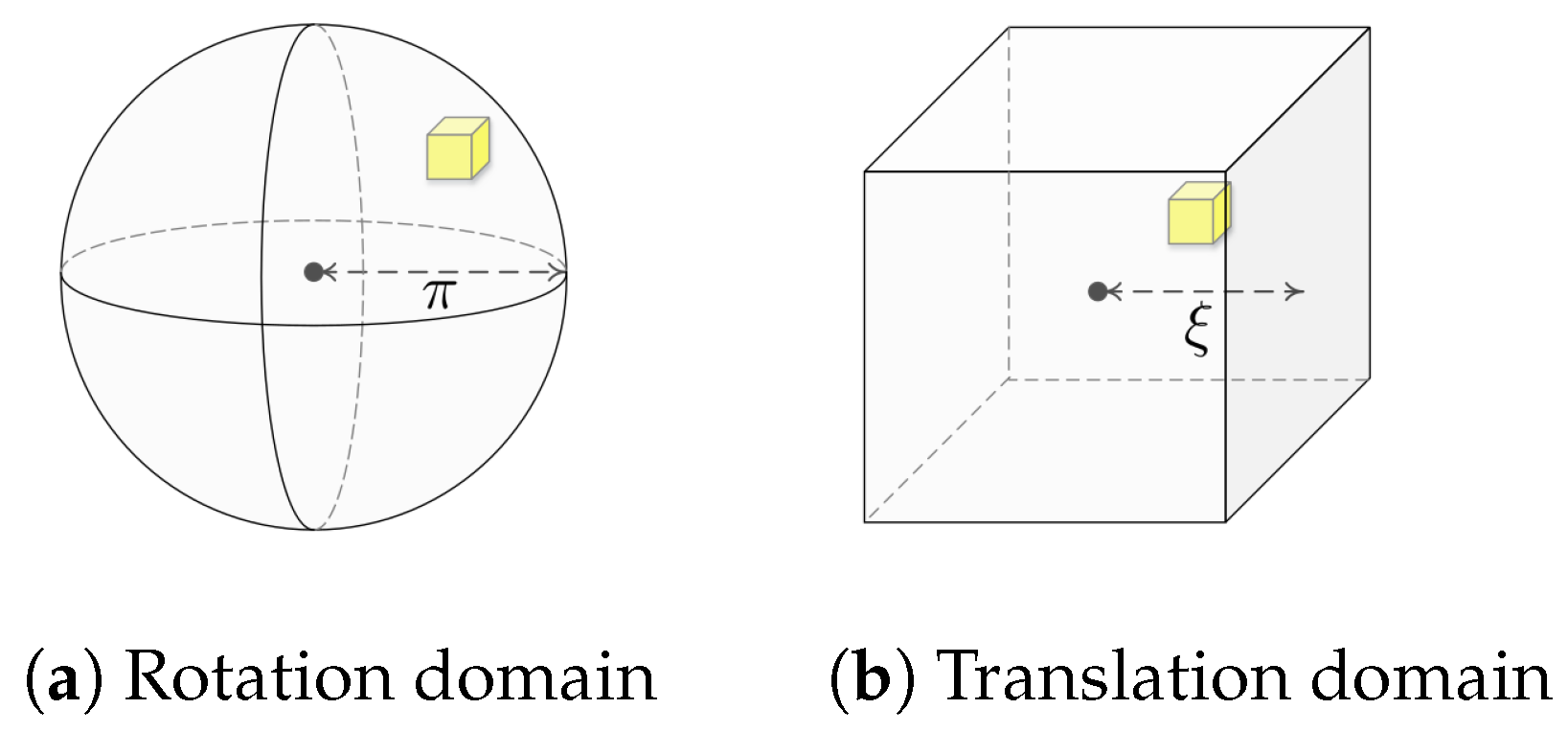
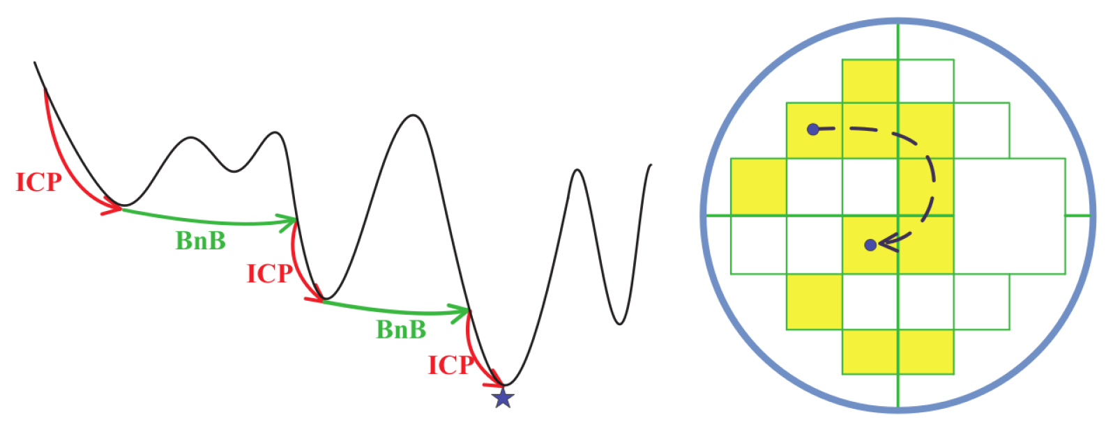
2.2. Go-ICP
2.3. Bayesian-ICP
2.4. Fast Point Feature Histograms
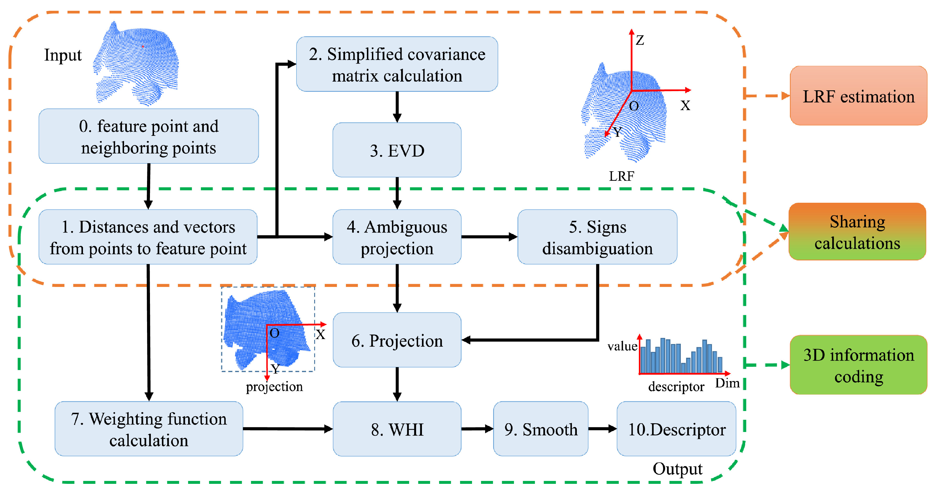
2.5. Weighted Height Image Descriptor
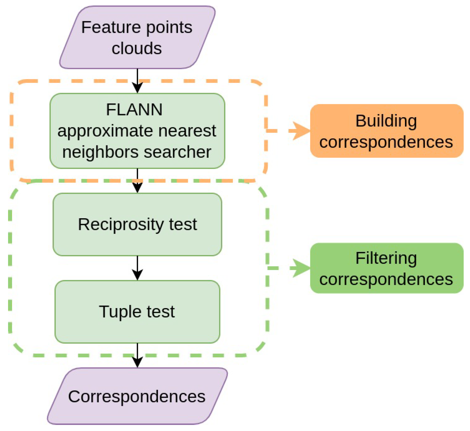
2.6. Fast Global Registration
2.7. Teaser++
- (1)
- Using TRIMs to estimate the scale ;
- (2)
- Using TIMs and to estimate the rotation ;
- (3)
- Using and to estimate translation from the TLS problem (11).
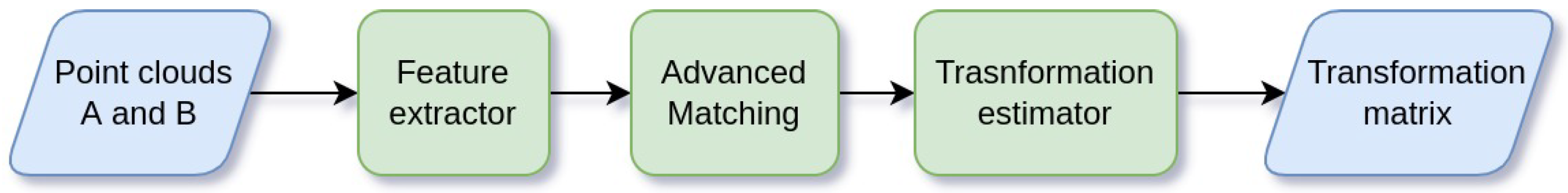
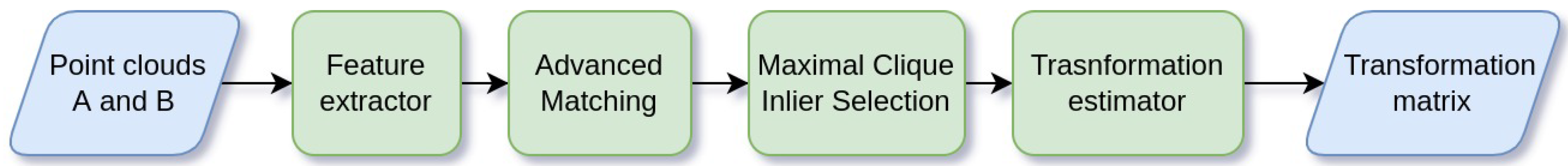
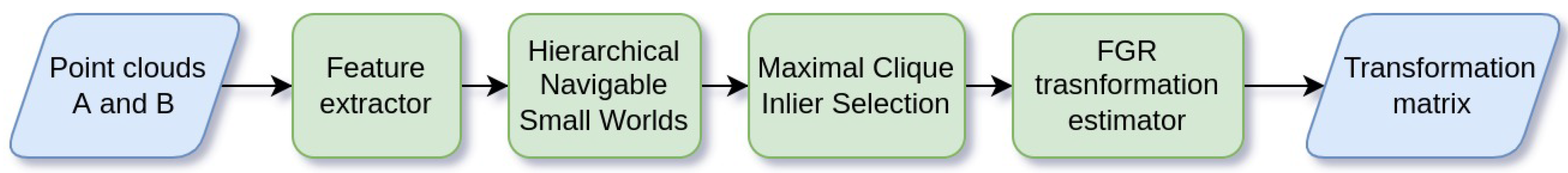
3. Feature Inliers Graph Registration Approach
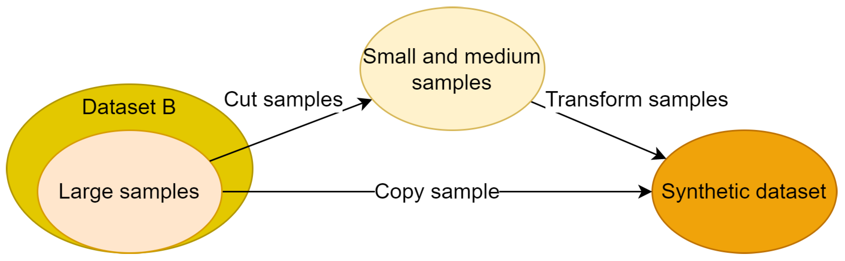
4. Datasets
5. Methodology
5.1. Efficiency Evaluation of Registration Algorithms
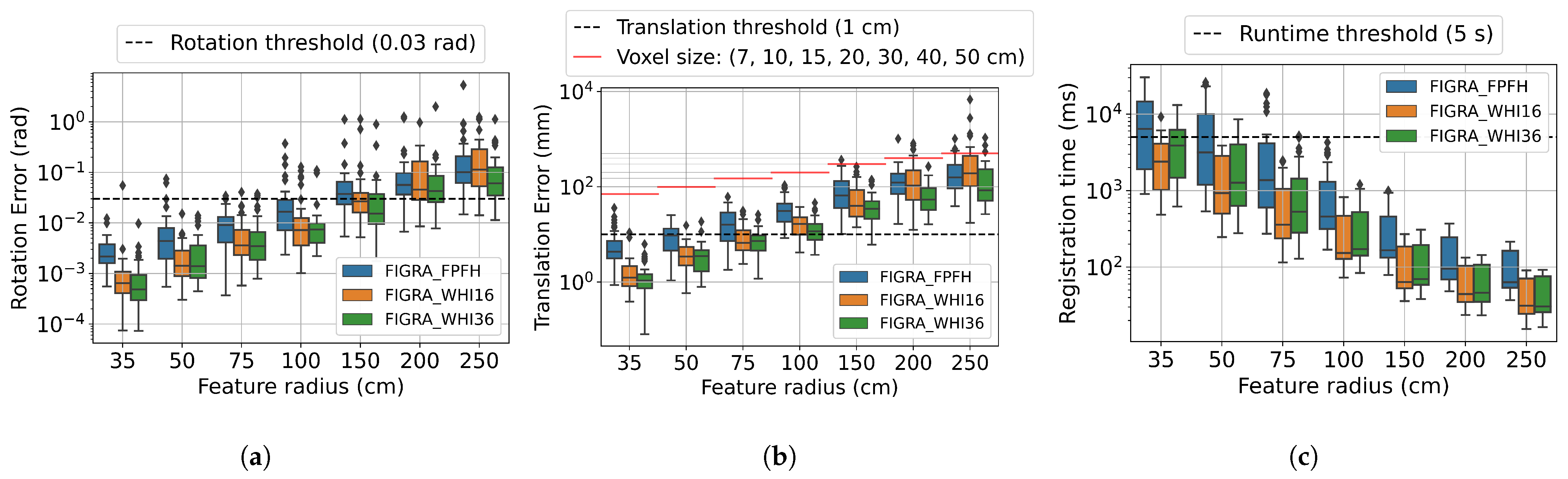
5.2. Accuracy and Runtime Analysis of Registration Methods: FGR, Teaser++, and FIGRA for Different Local Feature Descriptors
5.3. Accuracy and Runtime Analysis of Hybrid Approaches
6. Results
6.1. Efficiency Evaluation of Registration Algorithms on Real Datasets
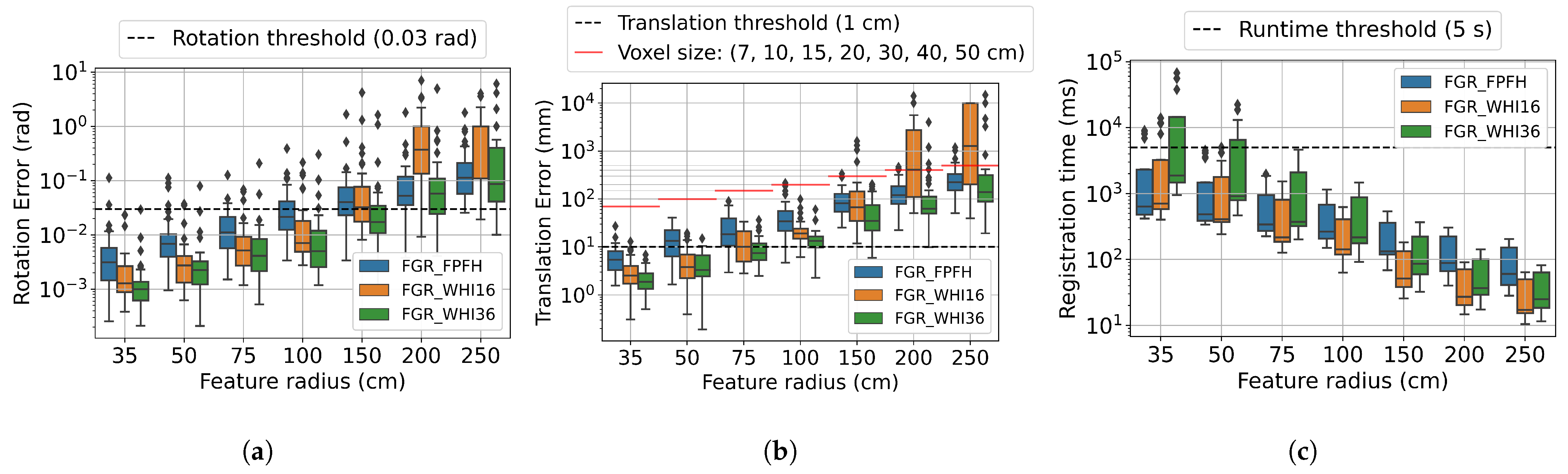
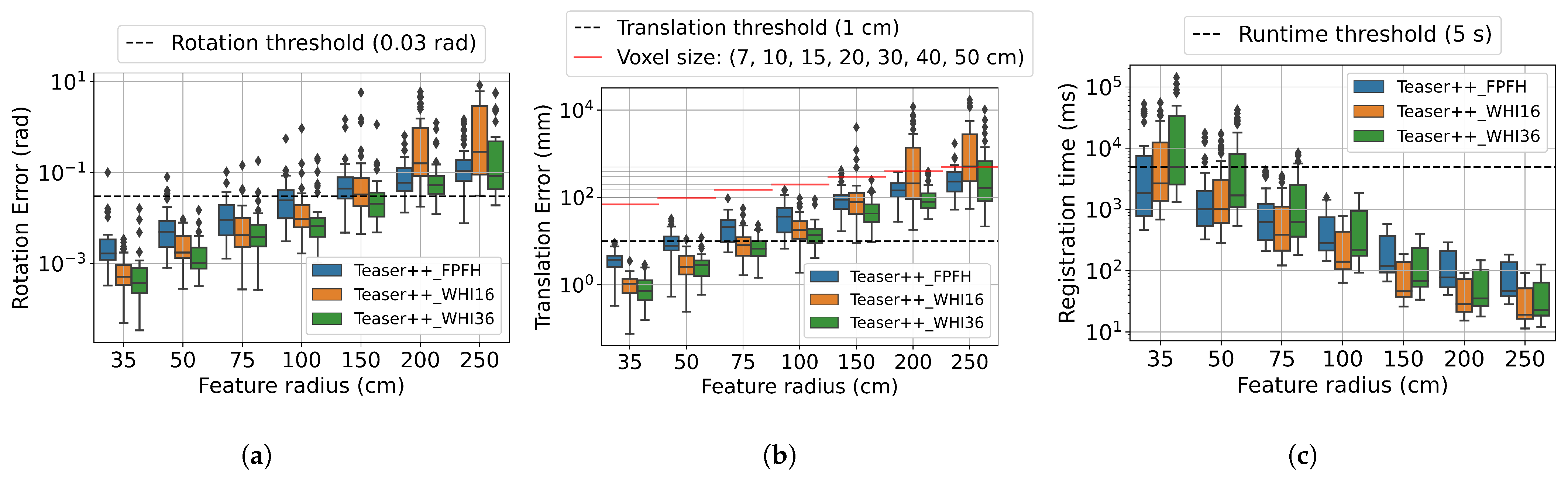
6.2. Accuracy and Runtime Analysis of FGR, Teaser++, and FIGRA for Different Feature Descriptors
6.3. Accuracy and Runtime Analysis of Hybrid Approaches: FGR, Teaser++, and FIGRA with ICP
7. Discussion
8. Conclusions
Author Contributions
Funding
Data Availability Statement
Conflicts of Interest
References
- Vidal-Balea, A.; Blanco-Novoa, Ó.; Fraga-Lamas, P.; Fernández-Caramés, T.M. Developing the next generation of augmented reality games for pediatric healthcare: An open-source collaborative framework based on arcore for implementing teaching, training and monitoring applications. Sensors 2021, 21, 1865. [Google Scholar] [CrossRef]
- Sydorenko, T.; Thorne, S.L.; Hellermann, J.; Sanchez, A.; Howe, V. Localized globalization: Directives in augmented reality game interaction. Mod. Lang. J. 2021, 105, 720–739. [Google Scholar] [CrossRef]
- Ladwig, P.; Geiger, C. A literature review on collaboration in mixed reality. In Smart Industry & Smart Education. REV 2018. Lecture Notes in Networks and Systems; Springer: Cham, Switzerland, 2018; pp. 591–600. [Google Scholar]
- Mourtzis, D.; Angelopoulos, J.; Panopoulos, N. Collaborative manufacturing design: A mixed reality and cloud-based framework for part design. Procedia CIRP 2021, 100, 97–102. [Google Scholar] [CrossRef]
- Garbett, J.; Hartley, T.; Heesom, D. A multi-user collaborative BIM-AR system to support design and construction. Autom. Constr. 2021, 122, 103487. [Google Scholar] [CrossRef]
- Rust, R.; Vasey, L.; Gramazio, F.; Kohler, M. Extended Reality Collaboration: Virtual and Mixed Reality System for Collaborative Design and Holographic-Assisted On-site Fabrication. In Towards Radical Regeneration: Design Modelling Symposium Berlin 2022; Springer Nature: Berlin/Heidelberg, Germany, 2022; p. 283. [Google Scholar]
- Prabhakaran, A.; Mahamadu, A.M.; Mahdjoubi, L.; Boguslawski, P. BIM-based immersive collaborative environment for furniture, fixture and equipment design. Autom. Constr. 2022, 142, 104489. [Google Scholar] [CrossRef]
- Ređep, T.; Hajdin, G. Use of Augmented Reality with Game Elements in Education–Literature Review. J. Inf. Organ. Sci. 2021, 45, 473–494. [Google Scholar]
- Bork, F.; Lehner, A.; Eck, U.; Navab, N.; Waschke, J.; Kugelmann, D. The effectiveness of collaborative augmented reality in gross anatomy teaching: A quantitative and qualitative pilot study. Anat. Sci. Educ. 2021, 14, 590–604. [Google Scholar] [CrossRef] [PubMed]
- Sáez-López, J.M.; Sevillano-García, M.L.; Pascual-Sevillano, M.A. Application of the ubiquitous game with augmented reality in Primary Education. Comunicar 2022, 61, 71–82. [Google Scholar] [CrossRef]
- Jacob, J.; Nóbrega, R. Collaborative augmented reality for cultural heritage, tourist sites and museums: Sharing Visitors’ experiences and interactions. In Augmented Reality in Tourism, Museums and Heritage; Springer: Berlin/Heidelberg, Germany, 2021; pp. 27–47. [Google Scholar]
- Microsoft. Azure Spatial Anchors. 2019. Available online: https://azure.microsoft.com/en-us/services/spatial-anchors/ (accessed on 11 November 2022).
- Niantic. Niantic Lightship. 2015. Available online: https://lightship.dev/ (accessed on 11 November 2022).
- Developers, G. Share AR Experiences with Cloud Anchors|ARCore. 2018. Available online: https://developers.google.com/ar/develop/java/cloud-anchors/overview-android (accessed on 11 November 2022).
- Reimer, D.; Podkosova, I.; Scherzer, D.; Kaufmann, H. Colocation for SLAM-Tracked VR Headsets with Hand Tracking. Computers 2021, 10, 58. [Google Scholar] [CrossRef]
- Dusmanu, M.; Miksik, O.; Schönberger, J.L.; Pollefeys, M. Cross-Descriptor Visual Localization and Mapping. In Proceedings of the IEEE/CVF International Conference on Computer Vision, Montreal, BC, Canada, 10–17 October 2021; pp. 6058–6067. [Google Scholar]
- Ng, P.C.; Henikoff, S. SIFT: Predicting amino acid changes that affect protein function. Nucleic Acids Res. 2003, 31, 3812–3814. [Google Scholar] [CrossRef] [PubMed] [Green Version]
- Tian, Y.; Yu, X.; Fan, B.; Wu, F.; Heijnen, H.; Balntas, V. Sosnet: Second order similarity regularization for local descriptor learning. In Proceedings of the IEEE/CVF Conference on Computer Vision and Pattern Recognition, Long Beach, CA, USA, 16–17 June 2019; pp. 11016–11025. [Google Scholar]
- Sun, T.; Liu, G.; Liu, S.; Meng, F.; Zeng, L.; Li, R. An efficient and compact 3D local descriptor based on the weighted height image. Inf. Sci. 2020, 520, 209–231. [Google Scholar] [CrossRef]
- Rusu, R.B.; Blodow, N.; Beetz, M. Fast point feature histograms (FPFH) for 3D registration. In Proceedings of the 2009 IEEE International Conference on Robotics and Automation, Kobe, Japan, 12–17 May 2009; pp. 3212–3217. [Google Scholar]
- Besl, P.J.; McKay, N.D. Method for registration of 3-D shapes. In Sensor Fusion IV: Control Paradigms and Data Structures; International Society for Optics and Photonics: Bellingham, WA, USA, 1992; Volume 1611, pp. 586–606. [Google Scholar]
- Morrison, D.R.; Jacobson, S.H.; Sauppe, J.J.; Sewell, E.C. Branch-and-bound algorithms: A survey of recent advances in searching, branching, and pruning. Discret. Optim. 2016, 19, 79–102. [Google Scholar] [CrossRef]
- Yang, J.; Li, H.; Campbell, D.; Jia, Y. Go-ICP: A globally optimal solution to 3D ICP point-set registration. IEEE Trans. Pattern Anal. Mach. Intell. 2015, 38, 2241–2254. [Google Scholar] [CrossRef] [PubMed] [Green Version]
- Maken, F.A.; Ramos, F.; Ott, L. Speeding up iterative closest point using stochastic gradient descent. In Proceedings of the 2019 International Conference on Robotics and Automation (ICRA), Montreal, QC, Canada, 20–24 May 2019; pp. 6395–6401. [Google Scholar]
- Welling, M.; Teh, Y.W. Bayesian learning via stochastic gradient Langevin dynamics. In Proceedings of the 28th international conference on machine learning (ICML-11), Bellevue, WA, USA, 28 June–2 July 2011; pp. 681–688. [Google Scholar]
- Guo, Y.; Bennamoun, M.; Sohel, F.; Lu, M.; Wan, J.; Kwok, N.M. A comprehensive performance evaluation of 3D local feature descriptors. Int. J. Comput. Vis. 2016, 116, 66–89. [Google Scholar] [CrossRef]
- Zhou, Q.Y.; Park, J.; Koltun, V. Fast global registration. In Proceedings of the European Conference on Computer Vision, Amsterdam, The Netherlands, 11–14 October 2016; Springer: Berlin/Heidelberg, Germany, 2016; pp. 766–782. [Google Scholar]
- Muja, M.; Lowe, D.G. Fast approximate nearest neighbors with automatic algorithm configuration. In Proceedings of the VISAPP 2009, Lisboa, Portugal, 5–8 February 2009; Volume 2, p. 2. [Google Scholar]
- Black, M.J.; Rangarajan, A. On the unification of line processes, outlier rejection, and robust statistics with applications in early vision. Int. J. Comput. Vis. 1996, 19, 57–91. [Google Scholar] [CrossRef]
- Yang, H.; Carlone, L. A polynomial-time solution for robust registration with extreme outlier rates. arXiv 2019, arXiv:1903.08588. [Google Scholar]
- Yang, H.; Antonante, P.; Tzoumas, V.; Carlone, L. Graduated non-convexity for robust spatial perception: From non-minimal solvers to global outlier rejection. IEEE Robot. Autom. Lett. 2020, 5, 1127–1134. [Google Scholar] [CrossRef] [Green Version]
- Yang, H.; Shi, J.; Carlone, L. Teaser: Fast and certifiable point cloud registration. IEEE Trans. Robot. 2020, 37, 314–333. [Google Scholar] [CrossRef]
- Malkov, Y.A.; Yashunin, D.A. Efficient and robust approximate nearest neighbor search using hierarchical navigable small world graphs. IEEE Trans. Pattern Anal. Mach. Intell. 2018, 42, 824–836. [Google Scholar] [CrossRef] [PubMed] [Green Version]
- Wang, M.; Xu, X.; Yue, Q.; Wang, Y. A comprehensive survey and experimental comparison of graph-based approximate nearest neighbor search. arXiv 2021, arXiv:2101.12631. [Google Scholar] [CrossRef]
- Point Cloud Library (PCL). 2022. Available online: https://pointclouds.org/ (accessed on 1 January 2023).


| Code | Name | Collecting Device | Type Data | Point Cloud Density | Environments |
|---|---|---|---|---|---|
| Dataset A | KTH Longterm | Scitos G5 robot with an RGB-D camera sensor | Point cloud indoor environment reconstructed by different SLAM algorithms | Dense | 4 rooms, 4 corridors |
| ICL-NUIM | RGB-D camera | 2 rooms | |||
| Dataset B | Indoor HoloLens | HoloLens glasses 1st and 2nd gen. | Sparse | 3 rooms, 1 corridor |
| Method | Feature | Advanced Matching | Average Runtime (ms) | Alignment Success (%) |
|---|---|---|---|---|
| Go-ICP | - | - | 24427 | 8 |
| Bayesian-ICP | - | - | 1647 | 54 |
| FGR | FPFH | 390 | 100 | |
| WHI16 | On | 371 | 100 | |
| WHI36 | 752 | 100 | ||
| FPFH | 442 | 100 | ||
| WHI16 | Off | 441 | 100 | |
| WHI36 | 823 | 92 | ||
| Teaser++ | FPFH | 409 | 100 | |
| WHI16 | On | 428 | 100 | |
| WHI36 | 823 | 100 | ||
| FPFH | 1847 | 100 | ||
| WHI16 | Off | 1209 | 100 | |
| WHI36 | 1897 | 100 | ||
| FIGRA | FPFH | 1359 | 100 | |
| WHI16 | - | 613 | 100 | |
| WHI36 | 687 | 100 | ||
| Method | Feature | Advanced Matching | Average Runtime (ms) | Alignment Success (%) |
| Go-ICP | - | - | 24158 | 0 |
| Bayesian-ICP | - | - | 1564 | 5 |
| FGR | FPFH | 219 | 68 | |
| WHI16 | On | 223 | 53 | |
| WHI36 | 419 | 79 | ||
| FPFH | 259 | 42 | ||
| WHI16 | Off | 262 | 26 | |
| WHI36 | 458 | 42 | ||
| Teaser++ | FPFH | 219 | 63 | |
| WHI16 | On | 213 | 58 | |
| WHI36 | 446 | 63 | ||
| FPFH | 365 | 79 | ||
| WHI16 | Off | 382 | 100 | |
| WHI36 | 641 | 100 | ||
| FIGRA | FPFH | 350 | 89 | |
| WHI16 | - | 288 | 100 | |
| WHI36 | 311 | 100 |
 |
Disclaimer/Publisher’s Note: The statements, opinions and data contained in all publications are solely those of the individual author(s) and contributor(s) and not of MDPI and/or the editor(s). MDPI and/or the editor(s) disclaim responsibility for any injury to people or property resulting from any ideas, methods, instructions or products referred to in the content. |
© 2023 by the authors. Licensee MDPI, Basel, Switzerland. This article is an open access article distributed under the terms and conditions of the Creative Commons Attribution (CC BY) license (https://creativecommons.org/licenses/by/4.0/).
Share and Cite
Osipov, A.; Ostanin, M.; Klimchik, A. Comparison of Point Cloud Registration Algorithms for Mixed-Reality Cross-Device Global Localization. Information 2023, 14, 149. https://doi.org/10.3390/info14030149
Osipov A, Ostanin M, Klimchik A. Comparison of Point Cloud Registration Algorithms for Mixed-Reality Cross-Device Global Localization. Information. 2023; 14(3):149. https://doi.org/10.3390/info14030149
Chicago/Turabian StyleOsipov, Alexander, Mikhail Ostanin, and Alexandr Klimchik. 2023. "Comparison of Point Cloud Registration Algorithms for Mixed-Reality Cross-Device Global Localization" Information 14, no. 3: 149. https://doi.org/10.3390/info14030149