

Transferring CNN Features Maps to Ensembles of Explainable Neural Networks

Department of Computer Science, University of Applied Sciences and Arts of Western Switzerland, Rue de la Prairie 4, 1202 Geneva, Switzerland
Information 2023, 14(2), 89; https://doi.org/10.3390/info14020089
Submission received: 11 November 2022
/
Revised: 31 January 2023
/
Accepted: 1 February 2023
/
Published: 2 February 2023
(This article belongs to the Special Issue Foundations and Challenges of Interpretable ML)
Abstract
:The explainability of connectionist models is nowadays an ongoing research issue. Before the advent of deep learning, propositional rules were generated from Multi Layer Perceptrons (MLPs) to explain how they classify data. This type of explanation technique is much less prevalent with ensembles of MLPs and deep models, such as Convolutional Neural Networks (CNNs). Our main contribution is the transfer of CNN feature maps to ensembles of DIMLP networks, which are translatable into propositional rules. We carried out three series of experiments; in the first, we applied DIMLP ensembles to a Covid dataset related to diagnosis from symptoms to show that the generated propositional rules provided intuitive explanations of DIMLP classifications. Then, our purpose was to compare rule extraction from DIMLP ensembles to other techniques using cross-validation. On four classification problems with over 10,000 samples, the rules we extracted provided the highest average predictive accuracy and fidelity. Finally, for the melanoma diagnostic problem, the average predictive accuracy of CNNs was 84.5% and the average fidelity of the top-level generated rules was 95.5%. The propositional rules generated from the CNNs were mapped at the input layer by squares in which the relevant data for the classifications resided. These squares represented regions of attention determining the final classification, with the rules providing logical reasoning.
1. Introduction
Deep neural networks (DNNs) are at the core of the considerable progress achieved recently. Nevertheless, the explainability of connectionist models is nowadays an ongoing research issue, because in the long run, the acceptance of these models will depend on it. DNN-based applications raise ethical and juridical barriers that restrain their acceptance by society. Their usefulness is frequently overshadowed by the impossibility to explain their decisions. Understanding the knowledge embedded within DNNs would help demystify Artificial Intelligence (AI) and enhance user confidence in these tools. Explainable AI (XAI) consists of AI methods that aim to explain why or how a model generates its results.
The capabilities of DNNs make them extremely useful for a wide variety of tasks. For example, critical systems that rely on autonomous decision-making mechanisms, such as automatic medical diagnosis, are difficult to certify because they cannot be tested in all possible circumstances and contexts. The ability to explain system decisions in a holistic manner would greatly facilitate the task of validating and certifying these systems for critical activities. Part of the current scepticism about intelligent autonomous systems is their inability to interact with humans. Transparent systems that can interact with the user and justify their actions would probably be much more welcome.
Interpretability and explainability are often used synonymously in the literature [1]. Furthermore, a mathematical definition of interpretability has not yet been formulated [1]. Namatevs et al. defined interpretability as follows: “Interpretability means the ability for a human to understand and trust the decision of the deep learning model’s results” [1]. A good explanation is interpretable and faithful [2], with faithfulness involving an accurate characterization of the behavior of a model. As a consequence, Namatevs et al. defined explainability as follows: “Explainability means the ability by which a human can justify the cause of the explanatory rule of the DL model’s results” [1].
Data are said to be tabular if it is possible to organize it in tables, i.e., in rows and columns where each type of information is always placed in the same place. The images are not tabular, because the same object could be in several different places. For tabular data, DNNs do not provide a clear benefit over well-established Machine Learning (ML) models, such as Multi Layer Perceptrons (MLPs), Support Vector Machines (SVMs), an ensemble of models, etc. A number of scholars attempted to explain the knowledge incorporated in MLPs and SVMs by propositional rules. Andrews et al. presented a comprehensive overview of rule extraction techniques to explain neural network (NN) responses [3]. For SVMs, a review of many explainability techniques was proposed in [4].
Models combined in an ensemble are often more accurate than a single model. Several learning methods for ensembles were proposed, such as bagging [5] and boosting [6]. However, even an MLP translatable into propositional rules loses its explainability when combined in an ensemble. Recently, a large number of XAI approaches have been introduced for DNNs, with the number of reviews constantly increasing [7]. Comprehensive overviews of XAI methods were presented in [8,9,10].
In this work, we propose a rule extraction technique applied to the various layers of a CNN. In that way, we determine the inference process that leads to classifications. Specifically, propositional rules are produced by transferring CNN feature maps to the Discretized Interpretable Multi Layer Perceptron (DIMLP) [11,12,13,14]. For this last model, the key idea of rule extraction is the identification of discriminative hyperplanes. In a DIMLP, each neuron in the first hidden layer receives a connection from a single input neuron. Thus, hyperplanes are not oblique but parallel to the axis of the input variables. The hyperplanes discriminate different classes based on the values of the weights after the first hidden layer. As a result, the input space is split into hyper-rectangles representing propositional rules. The production of rulesets is carried out by a greedy algorithm that determines whether hyperplanes are discriminative or not. For more details see [13].
After the training phase of a CNN, each feature map is used to train a DIMLP network. Finally, the outputs of these DIMLPs make it possible to constitute again a new dataset which is learned by a DIMLP ensemble. Therefore, at the low level we have many DIMLPs that learn CNN feature maps and at the top level lies a DIMLP ensemble that aggregates the DIMLP classifications obtained at a lower level. The rule extraction method is carried out from the DIMLPs in two steps. First, top-level rule extraction generates propositional rules that involve rule antecedents related to the outputs of low-level DIMLPs. Then, from the high-level rules, we generate low-level rules, with rule antecedents related to the CNN feature maps. In other words, we accomplish transfer learning of CNN feature maps to simpler models, such as DIMLPs. Thus, we do not explain the inference mechanism of a CNN, but rather the one of many DIMLPs in an ensemble. Our approach is viable, provided that our simplified model can be as accurate as the original CNN.
We performed three series of experiments. In the first, we applied DIMLP ensembles to a Covid dataset related to diagnosis from symptoms, to show how the generated propositional rules provide intuitive explanations of DIMLP classifications. Then, our purpose was to compare rule extraction from DIMLP ensembles to other techniques by cross-validation. On four classification problems with over 10,000 samples, the rules we extracted provided the highest average predictive accuracy. Finally, we applied transfer learning of CNN feature maps to DIMLP ensembles. CNNs were trained on images of melanoma and DIMLPs were as accurate as CNNs. The generated rules explaining DIMLP classifications were illustrated with several examples.
1.1. Related Work
Propositional rules include two parts: one or more rule antecedents and a conclusion. A rule antecedent is formally defined as , or ; with an input variable and a constant. Then, a propositional rule with k antecedents is: “if and … and then Conclusion”. In the context of data classification, “Conclusion” is a class. Golea showed that the explainability problem of MLPs by means of propositional rules is NP-hard [15]. Since Saito and Nakano’s early work on single MLPs [16], only a few authors tackled rule extraction from NN ensembles.
1.1.1. Rule Extraction from Ensembles of NNs
An algorithm for learning rules from ensembles of NNs was presented in [17]. In particular, NNs were used to generate additional data for rule learning. Additionally, continuous attributes were always discretized. The REFNE algorithm (Rule Extraction from NN Ensemble) was presented in [18]. With this approach, a trained ensemble produced supplementary samples and then generated propositional rules. Furthermore, attributes were discretized during rule extraction and it also used particular fidelity evaluation mechanisms. Finally, rules were limited to only three antecedents. An ensemble of simple Perceptrons was presented in [19]. By discretizing the inputs, propositional rules were produced from the oblique hyperplanes defined by the Perceptrons. With C4.5Rule-PANE, the C4.5 Decision Tree (DT) induction algorithm [20] builds a ruleset that imitated the inference process of a NN ensemble [21]. As in REFNE, additional instances were generated from the ensemble and rules were extracted from all those instances. In [22], a genetic programming approach was applied to derive rules from ensembles of 20 NNs. Rule extraction from ensembles was considered an optimization problem in which a trade-off between accuracy and comprehensibility is crucial. A rule extraction technique for a limited number of MLPs in an ensemble was introduced in [23,24]. Here, rule extraction was based on the Re-RX algorithm [25]. More recently, DIMLP ensembles were trained by optimizing their diversity [26], with rule extraction achieved for every single network in the ensemble. Then, for a given sample the rule that was chosen was the one with the highest confidence score. Finally, an algorithm named RE-E-NNES (Rule Extraction with Ensemble of NN Ensembles) used the C4.5 algorithm to extract rulesets from MLP ensembles trained by a boosting algorithm (NNBOOST), with at most ten MLPs [27]. RE-E-NNES generated rules from the first MLP, then with the second MLP these rules were refined and so on with the other MLPs.
A drawback of the rule extraction techniques presented in [17,18,19] is the discretization of continuous attributes, which need not be accomplished with DIMLP ensembles. Furthermore, in [18], rules were limited to three antecedents. With DIMLPs, there are no such limitations. In [19], the generated rules have linear combinations of the attributes in the antecedents. Thus, with a large number of variables, they are difficult to understand. For the techniques proposed in [21,27], it was observed in another work that the simple approach of adapting a DT to a DNN generally gives unsatisfactory results in terms of accuracy and fidelity [28]. The work presented in [22] focused on genetic algorithms. Although the latter represents an optimization algorithm capable of solving very complex problems, tuning the parameters is difficult due to its large number. With DIMLP ensembles, the rule extraction algorithm has no parameters to set. With the technique presented in [23,24], rule extraction was only defined for small ensembles, which could be a drawback when trying to achieve better results with large ensembles. With DIMLPs, the size of an ensemble is a parameter that can be set for small or large ensembles, which offers good flexibility.
1.1.2. Explainability with Deep Models
Several scholars presented local methods to explain the decisions taken by CNNs. Among these works, some have acquired a status of reference. For instance, the Local Interpretable Model-Agnostic Explanations (LIME) is a method that produces local explanations by fitting a transparent model around a single observation, capturing how the model behaves at that locality [29]. Shapley values are used in another well-established local explanation technique called SHAP that quantifies the contribution of features to a given model prediction [30]. In addition, Grad-CAM provides saliency maps that use the gradient flowing into the final convolutional layer to highlight class-relevant regions in the input [31].
Frosst and Hinton proposed a particular DT that imitated the input-output associations [32]. However, the DT did not explain the network logic, clearly. Another work proposed a DT that determined with respect to the images, which filters were activated by the portions of the object and to what extent they contributed to the final classification [33]. The Explainable Deep Neural Network (xDNN) was proposed in [34]. Essentially, it is an MLP that combines reasoning with respect to prototypes. Each generated rule antecedent represents the similarity to a prototype, which can be a training sample. With DeconvNet, strong activations were propagated backwards to determine the parts of the images that caused the activations [35]. An optimization technique based on image priors to invert a CNN was proposed to visualize the information represented at each layer [36]. Layer-wise Relevance Propagation (LRP) is a technique that determines heatmaps of relevant areas contributing to the final classification [37].
The main disadvantage of local algorithms such as LIME is their inability to grasp a process in its entirety. SHAP is used for local or global explanations. Nevertheless, a drawback is a computational complexity, which is exponential [38]. Furthermore, the characterization of the contribution of the variables to the outcome does not allow for a precise explanation of the reasoning of the model. For the explanation methods that generate maps (LRP, DeconvNet, and CNN inversion), how discrimination between different classes is carried out remains undetermined [2]. Note that this is also true for the relevance of variables to the outcome (SHAP). One of the qualities of xDNN is that the generated rules express a form of neural network reasoning with respect to the similarity of prototypes. Therefore, for the explainability of CNNs, we prefer to generate propositional rules because classes are precisely characterized by logical reasoning. The difference between our approach and xDNN is that the antecedents of our rules represent the pixel values of the feature maps, which allows us to determine the relevant pixel squares in the input images. Table 1 gives a summary of the methods described, with their characteristics.
2. Materials and Methods
In this work, the key idea is the transfer of CNN feature maps to an explainable model, such as DIMLP ensembles. So, we define a model based on DIMLPs with two hierarchical levels. At the lowest, many single DIMLPs learn the feature maps of a trained CNN. On top of these networks, a DIMLP ensemble aggregates all the lowest level DIMLP classifications. Rule extraction is achieved in two steps. First, propositional rules are generated from the DIMLP ensemble at the highest level and then secondary rules are derived from the DIMLPs that have been trained on the CNN feature maps.
2.1. MLP and DIMLP
2.1.1. MLP
MLPs are made of consecutive layers of neurons, with as a vector denoting the input layer. For layer , the activation values of the neurons are given by
is a matrix of weight parameters between two successive layers l and , is a vector also called the bias and is an activation function. For , we use here a sigmoid :
2.1.2. DIMLP
A Discretized Interpretable Multi Layer Perceptron is very similar to an MLP. In fact, as a small difference, is a diagonal matrix. Moreover, the activation function applied to is a staircase function . Here approximates with stairs a sigmoid function:
represents the abscissa of the first stair. By default .
represents the abscissa of the last stair. By default . Between and , is:
For , DIMLP and MLP are the same models.
In a DIMLP, for a classification problem, the input space is partitioned into hyper-rectangles representing propositional rules [13]. The staircase activation function and the diagonal matrix allow us to determine the precise location of axis-parallel hyperplanes representing the antecedents of the rules [13]. For each input neuron, the number of discriminant hyperplanes is at most equal to the number of stairs in the staircase activation function. The rule extraction algorithm first builds a decision tree with at each node a hyperplane; when then the tree is completed, each path from the root to a leaf represents a propositional rule. Finally, a greedy algorithm progressively removes antecedents and rules [13]. Its computational complexity is polynomial [14]; specifically, with S samples and V input variables it is O.
2.2. Ensembles
The accuracy of several combined models is often higher than that provided by a single model. Two important representative learning algorithms for ensembles are bagging [5] and boosting [6]. They have been applied to both DTs and NNs. In this work, we use DIMLP ensembles trained by bagging [5] and arcing [39], which is a simplified form of boosting. Recently, DIMLP ensembles were compared to ensembles of DTs trained by bagging and boosting [40], with DIMLPs achieving good predictive accuracy.
Bagging and arcing are rooted in resampling methods. With p training samples, bagging selects for each classifier p samples drawn with replacement from the original training set. Hence, many of the generated samples may be repeated while others may be left out. As a result, the individual models are slightly different and this proves beneficial compared to the combined ensemble of classifiers.
With arcing, a selection probability is associated with each training sample. Before training, all training samples are assigned the same probability (). Then, after the first classifier has been trained, the probability of selecting a sample from a new training set is increased for all unlearned samples and decreased for the others. Rule extraction from DIMLP ensembles is performed with the same algorithm applied to a single network since an ensemble can be represented by a single DIMLP network with an additional hidden layer [14].
2.3. Convolutional Neural Networks
2.3.1. Architecture
In CNNs, the convolution operator is fundamental. Considering two-dimensional convolution operator applied to images, given a two-dimensional kernel of size PxQ and a data matrix of elements , the calculation of an element of a convolutional layer is
with an activation function and the bias. Here, for we use the ReLU (Rectified Linear Unit):
Another important operator in CNNs is max-pooling. It reduces the size of a matrix by applying a “Max” operator over non-overlapping regions. For instance, if we apply the Max-pooling operator defined with blocks of size , with the following matrix the result is a scalar equal to 9.
In a CNN, one typically stacks a number of convolutional and Max-pooling layers and then stacks dense layers. The lower layers operate like feature extractors, which are then processed by the dense layers representing an MLP.
2.3.2. Transferring Featrure Maps to DIMLPs
Let us denote D as a dataset. For each sample of D, Equation (6) puts into play a feature map. Hence, with all the samples in D, each feature map is associated with a new dataset ; with k representing the index of the feature maps (; is the total number of feature maps.). Since DIMLPs are explainable models and our main purpose is explainability, the key idea is to learn each dataset with a DIMLP network . For all the feature maps of a CNN, we obtain an ensemble of DIMLPs, with each DIMLP trained on a different dataset. Each network is a weak learner, but our hope is that the ensemble of all the becomes a strong learner that is as accurate as a CNN. Figure 1 depicts the idea of transferring each CNN feature map to a DIMLP network that must be trained.
Once the networks have been trained, the question arising is how to combine their outputs to obtain a classification. For clarity, let us define the output vector of the DIMLP network :
depicts the output layer vector of , designates the sample of dataset ; with j representing the columns, since before the flattening it is a 2D feature map. Moreover, let us define as
is a vector representing all the outputs provided by all the , as shown by Figure 2. In addition, let us define as the components of the vectors; with (with the number of components). To summarize, for each sample of the original dataset D used to train a CNN, we can build a new data matrix representing all the vectors. Finally, is used to train another explainable model, which is again a DIMLP ensemble denoted as E.
The rule extraction technique presented here first generates propositional rules from E trained with dataset and then rules are produced from the lower layers with networks and datasets . Specifically, the rules generated from E involve in the antecedents the outputs of the weak learners , which in turn represent the probabilities of each class in a given classification problem. This is of interest to characterize the way the interacts to classify data, which also represents explainability at a higher level of abstraction.
To obtain rules from the feature maps, we go backwards from the E ensemble to the networks. Each rule antecedent generated from E defines a new classification problem with respect to a network and a dataset. Note that for each new classification problem, the positive class is defined when a rule antecedent generated from E is true and negative otherwise. As an example, suppose that from E we generate a rule with an antecedent given as , meaning that the probability of a class corresponding to a certain output neuron of a network is above 0.8; then, to generate the rules from a network we must add two additional layers of neurons, as shown by Figure 3. Their role is to define a new class when it is true that and another when .
In Figure 3, the first additional layer with a unique neuron detects whether the activation is above threshold . When it occurs, neuron at the top is very close to one after the sigmoid is applied and neuron is very close to zero. Otherwise, is close to zero and is close to one. Likewise, it is possible to code a rule antecedent such as by different weight values of the last two layers. In this way, rules are generated from the networks, with the antecedents of the rules representing the features of the CNN at different convolution levels.
3. Results
We performed the experiments in three parts. First, we presented a classification problem on a COVID-19 diagnosis to illustrate examples of generated propositional rules. In the second part, we assessed the performance of our ensemble models by cross-validation on four classification problems with more than 10,000 samples. In the last part of the experiments, we applied CNNs to a melanoma diagnosis problem, then we transferred the CNN feature maps to DIMLP ensembles and finally we generated propositional rules.
Table 2 illustrates the main characteristics of several retrieved datasets from two sources: the Machine Learning Repository at the University of California, Irvine [41] (MLR-UCI) and the Kaggle platform.
Training sets were normalized by Gaussian normalization. All DIMLP ensembles were trained by back-propagation with default learning parameters:
- Learning parameter = 0.1;
- Momentum = 0.6;
- Flat Spot Elimination = 0.01;
- Number of stairs in the staircase activation function = 50.
Since predictive accuracy is defined as the ratio of the number of correctly classified samples to the total number of samples in a test set [42], the Tables of the results include:
- Average predictive accuracy of the model;
- Average fidelity on the testing set, which is the degree of matching between the generated rules and the model. Specifically, with P samples in the test set and Q samples for which the classifications of the rules match the classifications of the model, the fidelity is ;
- Average predictive accuracy of the rules;
- Average predictive accuracy of the rules when rules and model agree. Specifically, it is the proportion of correctly classified samples among the Q samples defined above;
- Average number of extracted rules;
- Average number of rule antecedents.
3.1. Experiments with a COVID-19 Dataset
Our aim here is to illustrate an example of the explainability of neural models with a particular classification problem in COVID-19 detection. The total number of samples in the used dataset is 5434, where COVID-19 positive samples were 4383 and COVID-19 negative samples were 1051 [43]. Twenty Boolean variables representing symptoms or observations were defined, such as absence/presence of: dry cough; fever; breathing problems; runny nose; abroad travel; etc. DIMLP architectures were defined with two hidden layers. The default number of neurons in the first hidden layer was equal to the number of input neurons. For the second hidden layer, this number was defined empirically, in order to obtain a number of connections less than or similar to the number of training samples. Consequently, the number of neurons in the second hidden layer was set to 100. Finally, out-of-bag samples were used to avoid the overtraining phenomenon, by applying an early-stopping technique. Specifically, the out-of-bag set constitutes a subset of the training dataset that is not used to fit the weight values of the NNs.
We carried out experiments based on ten repetitions of stratified 10-fold cross-validation trials. Table 3 illustrates the results for arced ensembles of DIMLPs (DIMLP-AT) and bagged ensembles of DIMLPs (DIMLP-BT). The average predictive accuracy obtained by DIMLP-BT was higher than that provided by DIMLP-AT. In addition, the average complexity in terms of the number of rules and a number of rule antecedents was quite similar for both models. Finally, with this classification problem, the fidelity was perfect, with an average value equal to 100%.
Listing 1 illustrates an example of generated rules from DIMLP-BT during cross-validation trials. The predictive accuracy of this ruleset was 99.5%, with fifteen of the 27 rules presented here. The first rule says that if a person presents fever, a dry cough and a sore throat, then she/he is Covid positive. Rule ten means that someone who does not have problems breathing, who does not have a sore throat, who has not travelled abroad and who has not attended a large gathering is negative. All these rules are easy to understand and explain the classifications of DIMLP ensembles.
| Listing 1. Examples of rules generated from DIMLP-BT. Meaningful antecedents are represented in italics. The numbers in parenthesis represent the number of samples covered in the training set, with the rules ranked in descending order with respect to these. |
| Rule 1: IF AND AND THEN COVID (2551) |
| Rule 2: IF THEN COVID (2186) |
| Rule 3: IF AND THEN COVID (1908) |
| Rule 4: IF AND THEN COVID (1877) |
| Rule 5: IF AND THEN COVID (1725) |
| Rule 6: IF AND AND THEN COVID (1574) |
| Rule 7: IF AND AND AND THEN COVID (1141) |
| Rule 8: IF AND NOT AND THEN COVID (1140) |
| Rule 9: IF AND AND AND NOT THEN COVID (1074) |
| Rule 10: IF AND AND THEN COVID (770) |
| Rule 11: IF NOT AND NOT AND NOT AND NOT THEN NEGATIVE (511) |
| Rule 12: IF NOT AND NOT AND NOT THEN NEGATIVE (414) |
| Rule 13: IF NOT AND NOT AND NOT THEN NEGATIVE (382) |
| Rule 14: IF AND AND AND AND NOT THEN COVID (377) |
| Rule 15: IF NOT AND NOT AND NOT THEN NEGATIVE (351) |
Listing 2 shows how rules cover the test samples against the same ruleset presented above. The first row signifies that the first rule was activated by 308 test samples, with 306 correctly classified samples and two misclassified samples, resulting in 99.4% accuracy. Note that for many rules the predictive accuracy is 100%.
| Listing 2. Activations of the rules by the test samples of a cross-validation trial. From left to right, the columns show the rule number, the number of activations of the rule, the number of correctly classified samples, the number of wrongly classified samples, the resulting accuracy and the class of the rule. |
| Rule 1: 308 306 2 0.993506 Class = COVID |
| Rule 2: 265 265 0 1.000000 Class = COVID |
| Rule 3: 211 211 0 1.000000 Class = COVID |
| Rule 4: 210 210 0 1.000000 Class = COVID |
| Rule 5: 203 203 0 1.000000 Class = COVID |
| Rule 6: 174 173 1 0.994253 Class = COVID |
| Rule 7: 119 118 1 0.991597 Class = COVID |
| Rule 8: 137 136 1 0.992701 Class = COVID |
| Rule 9: 135 134 1 0.992593 Class = COVID |
| Rule 10: 93 93 0 1.000000 Class = COVID |
| Rule 11: 61 61 0 1.000000 Class = NEGATIVE |
| Rule 12: 43 43 0 1.000000 Class = NEGATIVE |
| Rule 13: 38 38 0 1.000000 Class = NEGATIVE |
| Rule 14: 43 43 0 1.000000 Class = COVID |
| Rule 15: 38 38 0 1.000000 Class = NEGATIVE |
| Rule 16: 37 37 0 1.000000 Class = NEGATIVE |
| Rule 17: 25 25 0 1.000000 Class = COVID |
| Rule 18: 25 24 1 0.960000 Class = NEGATIVE |
| Rule 19: 18 18 0 1.000000 Class = NEGATIVE |
| Rule 20: 21 21 0 1.000000 Class = NEGATIVE |
| Rule 21: 11 11 0 1.000000 Class = NEGATIVE |
| Rule 22: 17 17 0 1.000000 Class = NEGATIVE |
| Rule 23: 14 14 0 1.000000 Class = NEGATIVE |
| Rule 24: 8 8 0 1.000000 Class = COVID |
| Rule 25: 5 5 0 1.000000 Class = NEGATIVE |
| Rule 26: 5 5 0 1.000000 Class = COVID |
| Rule 27: 2 2 0 1.000000 Class = NEGATIVE |
3.2. Comparison with Other Explainability Methods
In [40], we performed a comparative study on rule extraction from DIMLP ensembles with eight classification problems of size less than 1000 samples. Overall, the rules extracted from the ensembles were very competitive with respect to other approaches. As we have almost never trained our NNs with more than 10,000 samples, we decided to apply the DIMLP ensembles to four datasets of this size. For comparison purposes, as in [44], we achieved experiments based on five repetitions of stratified five-fold cross-validation.
For DIMLPs, the number of neurons in the second hidden were the following:
- Chess: 200;
- Connect4: 40;
- EEG eye state: 100;
- Letter recognition: 200;
These numbers were again set so that the number of connections was less than the number of samples. Table 4 illustrates average results provided by DIMLP ensembles with standard deviations between brackets. For each classification problem, bold face indicates the highest average accuracy or fidelity, while for rules, bold depicts the lowest average with respect to their number and their number of antecedents per rule. Average fidelity was always over 90% and the average predictive accuracy of the extracted rules, when rules and ensembles agreed (fifth column) was higher than that obtained by the rules (fourth column). One possible explanation is that the test samples for which the extracted rules and the model disagreed were the most difficult samples to classify. Hence, when they were excluded, the average predictive accuracy improved.
The authors of [44] applied the Synthetic Minority Oversampling Technique (SMOTE) to the training datasets to upsample the minority classes [45]. For comparison purposes, we have also applied SMOTE to these classification problems. Table 5 illustrates the results. The average predictive accuracy and the average fidelity of the rules generated from DIMLP ensembles were substantially higher than that provided by C4.5-PANE [21] or Trepan [46]. In addition, the average number of rules extracted from DIMLP ensembles was lower than that generated by C4.5-PANE. For the EEG dataset, Trepan generated only two rules on average. The reason for this small number of rules is that Trepan is forced to generate small rulesets that must cover large areas of the input space [44]. Nevertheless, the average predictive accuracy provided by Trepan was much lower than that obtained by DIMLP ensembles.
3.3. Experiments with CNNs
We trained the CNNs ten times with a skin cancer dataset based on coloured images. The interested reader will find other tumour-related problems in [47,48,49]. The dataset includes a training set of 2637 samples and a test set of 660 samples with classes “Benign” and “Malignant”. The former class represents 54.6% of the training set and 54.5% of the testing set. A tuning set randomly selected from the training set consisting of 500 samples was used for early-stopping.
After preliminary experiments, we defined a NN architecture with four convolutional layers and three fully connected layers. Each convolutional layer was followed by a Max-Pooling layer. For clarity, here we summarize the architecture:
- 2D-Convolution with 32 kernels of size and ReLU activation function.
- Max-Pooling layer with blocks of size (32 units).
- 2D-Convolution with 32 kernels of size and ReLU activation function.
- Max-Pooling layer with blocks of size (32 units).
- 2D-Convolution with 32 kernels of size and ReLU activation function.
- Max-Pooling layer with blocks of size (32 units).
- 2D-Convolution with 32 kernels of size and ReLU activation function.
- Max-Pooling layer with blocks of size (32 units).
- Fully connected layer with sigmoid activation function (128 neurons).
- Fully connected layer with sigmoid activation function (64 neurons).
- Fully connected layer with sigmoid activation function (2 neurons).
After any convolutional layer or any Max-pooling layer, we have the feature maps. For instance, after the first convolutional layer, we have 32 feature maps of size and after the first Max-pooling layer, another 32 feature maps with a size of . We used all four layers of feature maps to train DIMLPs. Specifically, the first layer of feature maps was selected at the first Max-pooling layer, the second at the second Max-pooling layer, the third at the third Max-pooling layer, and the fourth at the fourth Max-pooling layer. Each feature map defines itself as a new training set that can be learned by a DIMLP with two hidden layers. For clarity, let us enumerate at the level of each feature map the number of DIMLP input neurons:
- First level of feature maps: 32 DIMLPs with inputs and five neurons in the second hidden layer (in the first hidden layer the number of neurons is the same as in the input layer).
- Second level of feature maps: 32 DIMLPs with inputs and ten neurons in the second hidden layer.
- Third level of feature maps: 32 DIMLPs with inputs and 30 neurons in the second hidden layer.
- Fourth level of feature maps: 32 DIMLPs with inputs and 50 neurons in the second hidden layer.
The number of hidden neurons in the second hidden layer of DIMLPs was empirically defined, after preliminary tests. In addition, for each DIMLP network, a tuning set represented by the same examples used to train each CNN was used for early stopping.
3.3.1. Extraction of Rules at the Top Level (E Ensemble Dataset)
After the trainng of the DIMLPs, we agregated all DIMLP outputs ( dataset, cf. Section 2.3.2). Since each DIMLP consists of two output neurons, we obtained 256 neurons representing the probability of the classes for each DIMLP network trained with a different feature map. With these new 256 variables, we trained DIMLP-BTs to determine whether the average predictive accuracy was comparable to that obtained with CNNs. This procedure was repeated ten times for both CNNs and DIMLP ensembles. Finally, we generated propositional rules, with the results shown in Table 6.
The average predictive accuracy provided by DIMLP-BT was slightly, but not significantly, higher than that obtained from CNNs (84.7% versus 84.5%). Thus, the transfer of CNN feature maps to a number of simpler models such as DIMLPs was successful. The average predictive accuracy of the rules was lower than that given by the CNNs (83.6% versus 84.5%), but whether this is statistically significant should be determined. We therefore performed a Wilcoxon sign rank test in which the null hypothesis was defined as follows: the difference between two 10-component data vectors has a median of zero. Note that the Wilcoxon signed-ranks test is a non-parametric equivalent of the paired t-test. In our case, we required a pairwise statistical test, as the generated rulesets depend on neural networks. The result of this statistical test did not reject the null hypothesis at the default 5% significance level (p-value ). Thus, the median of the differences was unlikely to be non-zero. We performed the same test replacing the first measure of rule accuracy with the second measure (mean 85.8%) This statistical test rejected the null hypothesis at the default 5% significance level (p-value ) Thus, in this case, it is unlikely that the median of the differences was zero. Table 7 shows the predictive accuracy of the models (CNN and DIMLP-BT) and the accuracy of the rules generated for ten trials from which the p-values shown above were calculated.
Listing 3 shows twelve rules out of 129 generated from high-level attributes ( dataset and DIMLP ensemble E). This ruleset correctly classified 85.3% of the testing samples, with a fidelity of 94.5%. Odd attributes are relative to the probability of the first class, while even attributes are relative to the second class. The number of possible antecedents is 256 (); those between one and 64 concern the DIMLP networks trained with the first level of feature maps (); those between 65 and 128 concern the DIMLP networks trained with the second level of feature maps (); etc.
| Listing 3. Example of rules generated from the highest level of abstraction ( dataset). Odd attributes are relative to the probability of the “Malignant” class, while even attributes are relative to the “Benign” class. |
| Rule 1: |
| Rule 2: |
| Rule 3: |
| Rule 4: |
| Rule 5: |
| Rule 6: |
| Rule 7: |
| Rule 8: |
| Rule 9: |
| Rule 10: |
| Rule 11: |
| Rule 12: |
3.3.2. Extraction of Rules at the Level of the CNN Feature Maps
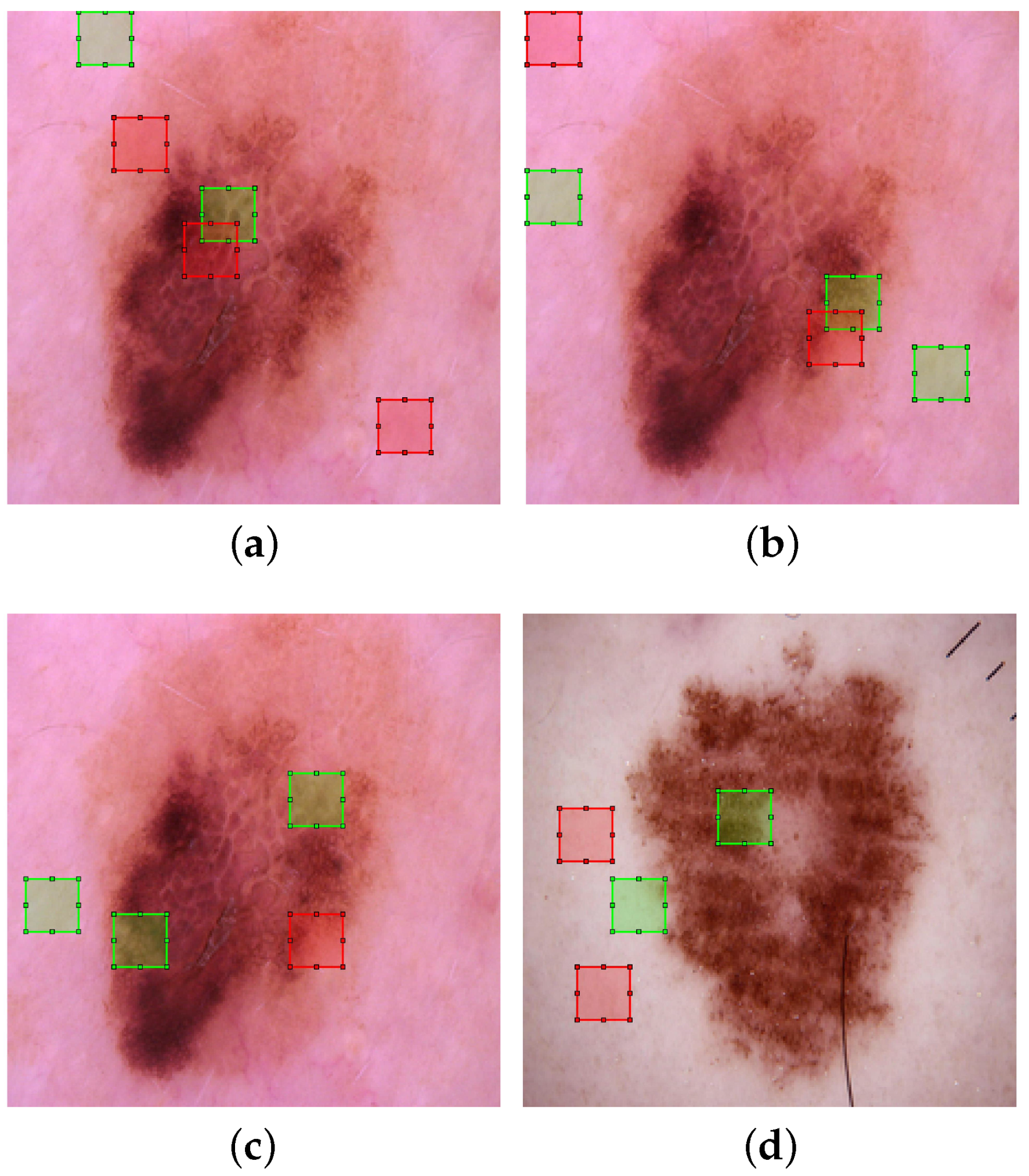
The first rule given above covered 206 testing samples and it was wrong only in two cases. Following the approach described in Section 2.3.2, the first antecedent yields five rules related to the feature maps that cover this sample. The five rules derived from have rule antecedents related to regions of size in the input layer. Specifically, these regions show where the convolution operator is applied, which in turn indicates where to look to understand the classification. Figure 4a depicts one of the five rules covering a particular testing sample, with five rule antecedents related to squares. In addition, green is for antecedents with “>” and red for those with “<”. It is worth noticing that three antecedents are in the background (on the left) and two in the centre representing a region of interest. These last two squares seem to be located in two homogeneous areas. A question arising here is why three antecedents related to the background are present in this rule. One reason could be that, as in other samples we find brownish areas in these places related to moles, some background/foreground discrimination has to be achieved.
The second antecedent of the first rule shown above is related to the fourth level of the feature maps. Thus, the size of the relevant regions in the input layer is of size . Figure 4b depicts a rule with five rule antecedents. We notice several antecedents related to the background and an antecedent related to the centre. The large squares are less informative, as it is then difficult to determine the points of the mole that determine the classification.
Another “Benign” sample covered by the first rule was taken into account. From antecedent , several rules were determined, including a rule with the three antecedents shown in Figure 4c. Specifically, two rule antecedents are related to the background and one is related to the mole. For the latter, the pixels of the square are rather uniform. Regarding antecedent , Figure 4d depicts the derived rule antecedents, with two of them related to the background and one covering almost the entire mole. Again, due to the size of the squares, is more informative than .
As an example of the “Malignant” rule, we consider the seventh rule shown in the third listing. It includes three rule antecedents related to the second level of the feature maps: ; ; and . This rule covers 78 samples of the testing set with an accuracy of 94.9%. As it was shown above, Figure 5a illustrates a rule derived from , the size of the squares being . Three squares are in the background, while two squares are close to the centre of the picture. In these latter squares, the uniformity of the texture seems to be less than that observed in the “Benign” cases presented above.
Figure 5b depicts a rule derived from , with two squares close to the border of the mole. Similarly, in Figure 5c, three squares are close to the borders and one is in the background. The pixels close to the border do not appear to be very uniform. Finally, Figure 5d–f illustrate another testing sample covered again by the seventh rule at the top level.
We applied Grad-CAM to the CNN network, which allowed us to produce the previous figures by DIMLPs. Figure 6a,b depict two samples of class “Benign”, with (c) and (d) showing two samples of class “Malignant”. Note that class-relevant regions in the images are highlighted with colours. Warm colours represent regions of relevance to the class, with colder colours indicating low relevance. At the top of the figure (a and b), the entire moles have high/moderate relevance, which is not very informative. For the sample in (c), we see two relevant areas at the top, outside the mole, which is probably not what we could expect. In (d), from the colours at the bottom right outside the mole, we see a highly relevant region. In addition, a large part of the mole appearing greenish is also relevant.
4. Discussion
In this work, we generated propositional rules from CNNs by performing transfer learning with DIMLPs. The proposed approach has three main steps. In the first step, each CNN feature map is used to train a single DIMLP network. Here, we had 128 feature maps that were learned by 128 DIMLPs. Then, in the second step, we trained a DIMLP ensemble (DIMLP-BT) with the outputs of the DIMLPs obtained in the first step. Specifically, with a binary classification problem, a DIMLP ensemble of 25 DIMLPs with 256 inputs was trained by bagging. In the third step, rule extraction was performed by extracting rules from DIMLP-BT, and then from these rules, other rules were produced against the feature maps.
Our approach to explaining CNN responses belongs to the category of global techniques and can be applied once all feature maps are available. In addition, our method is general with polynomial computational complexity. Note also that the learning of the feature maps can be executed in parallel. The results obtained are propositional rules that are linked in the antecedents to pixel squares where the convolution operators are applied. For a diagnostic application, specialists can inspect these squares to attempt an explanation. In the pictures above related to DIMLPs, we have seen rather uniform areas of attention for benign cases (e.g., small squares), while malignant examples have highlighted less uniform areas (for instance on the edges of moles). The state-of-the-art highlights a family of explainability methods based on saliency maps. The question then arises as to what makes our approach different. Essentially, we focused on regions of attention related to rule antecedents. Thus, to determine a sample classification, a logical inference is carried out, which is not the case with saliency maps. Regarding the limitations of our approach, the computational complexity is not linear; therefore, it cannot be applied to millions of data samples but only to a few thousand.
The size of the squares in which the data relevant to the classifications resided depended on the level of the feature maps. Thus, at the lowest level (after the input layer), their size was and at the highest level, it was equal to . For the larger squares, explainability is limited, since it could include a mole in its entirety without telling us in which part a possible anomaly would be found. It is worth noting that in the ruleset used to illustrate the images above, antecedents only associated with the fourth level of the feature maps were absent. Thus, each rule was also linked to small regions of attention. By qualitatively comparing our approach to Grad-CAM, we noticed that our method is more informative since the attention squares can be small and therefore more specific in targeting an anomaly. Moreover, the symbolic rules obtained make it possible to determine how the model “thinks” with respect to the pixels of the feature maps.
All the feature maps could have been transferred simultaneously, instead of transferring each map individually to a DIMLP network. The disadvantage of this alternative approach is that the dimension of the input layer would be very large and so the rule extraction algorithm would suffer in terms of computation time since its algorithmic complexity is polynomial. However, it would be possible to compress the feature maps by the Discrete Cosinus Transform (DCT), as we accomplished in [50].
5. Conclusions
With several classification problems, we have shown that DIMLP ensembles can generate more accurate rules with higher fidelity than other rule extraction methods. We therefore wondered whether it would have been possible to apply our approach to the CNNs. Specifically, we accomplished an indirect approach; that is, we transferred all the feature maps of a CNN to DIMLP networks that learned them. Then, the responses of all DIMLPs for each of the feature maps were aggregated and learned by a new ensemble of DIMLPs. On average, DIMLP ensembles were able to be as accurate as the original CNNs (84.7% versus 84.5%). Furthermore, the average fidelity of the top-level generated rules was 95.5%. Finally, the average predictive accuracy of the rules when DIMLP ensembles agreed with the rules was 85.8%.
In future work, we might consider training DIMLPs with all the attention squares related to the rule antecedents of the feature maps. In particular, for each propositional rule, all underlying attention squares would be used to train a DIMLP network. Compared to the approach proposed here, we would transfer the inputs of the attention areas and not the feature maps of the different convolution levels. When an area of attention is too large, we could use DCT to reduce the dimensionality. Once the DIMLP networks are trained, the responses representing the probabilities of class membership will be aggregated into a new ensemble, as in this work. In this way, propositional rules could be obtained with the pixels of the input layer as antecedents. This approach would be valid, provided that an accuracy close to that obtained by a CNN could be achieved.
Finally, it would be interesting to apply the proposed approach to pre-trained networks such as VGG, Resnet, etc. Since these models are even deeper, we would have to transfer a much larger number of feature maps. Rule extraction would be tractable provided that the number of examples remains limited to a few thousand, which is the case in many biological/medical problems.
Funding
This work was conducted in the context of the Horizon Europe project PRE-ACT (Prediction of Radiotherapy side effects using explainable AI for patient communication and treatment modification). It was supported by the European Commission through the Horizon Europe Program (Grant Agreement number 101057746), by the Swiss State Secretariat for Education, Research and Innovation (SERI) under contract number 22 00058, and by the UK government (Innovate UK application number 10061955).
Institutional Review Board Statement
Ethical review and approval were waived as all datasets used are publicly available.
Informed Consent Statement
Not Applicable.
Data Availability Statement
The “Chess”, “Connect4”, “EEG eye” and “Letter” datasets were retrieved from https://archive.ics.uci.edu/ml/index.php. The “COVID-19 symptoms” was retrieved from https://www.kaggle.com/hemanthhari/symptoms-and-covid-presence and the “Melanoma Diagnosis” from https://www.kaggle.com/fanconic/skin-cancer-malignant-vs-benign (all accessed on 1 September 2022).
Conflicts of Interest
The author declared no conflict of interest.
Abbreviations
The following abbreviations are used in this manuscript:
| AI | Artificial Intelligence |
| CNN | Convolutional Neural Network |
| DCT | Discrete Cosinus Transform |
| DIMLP | Discretized Interpretable Multi Layer Perceptron |
| DNNs | Deep neural network |
| DT | Decision Trees |
| IMLP | Interpretable Multi Layer Perceptrons |
| LIME | Interpretable Model-Agnostic Explanations |
| ML | Machine Learning |
| MLR-UCI | Machine Learning Repository at the University of California, Irvine |
| MLP | Multi Layer Perceptron |
| NN | Neural Network |
| SMOTE | Synthetic Minority Oversampling Technique |
| XAI | Explainable Artificial Intelligence |
| xDNN | Explainable Deep Neural Network |
References
- Namatēvs, I.; Sudars, K.; Dobrājs, A. Interpretability versus Explainability: Classification for Understanding Deep Learning Systems and Models. Comput. Assist. Methods Eng. Sci. 2022, 29, 297–356. [Google Scholar]
- Rudin, C. Please stop explaining black box models for high stakes decisions. arXiv 2018, arXiv:1811.10154. [Google Scholar]
- Andrews, R.; Diederich, J.; Tickle, A.B. Survey and critique of techniques for extracting rules from trained artificial neural networks. Knowl.-Based Syst. 1995, 8, 373–389. [Google Scholar] [CrossRef]
- Diederich, J. Rule Extraction from Support Vector Machines; Springer Science and Business Media: Berlin/Heidelberg, Germany, 2008; Volume 80. [Google Scholar] [CrossRef]
- Breiman, L. Bagging predictors. Mach. Learn. 1996, 24, 123–140. [Google Scholar] [CrossRef]
- Freund, Y.; Schapire, R.E. A desicion-theoretic generalization of on-line learning and an application to boosting. J. Comput. Syst. Sci. 1997, 55, 119–139. [Google Scholar] [CrossRef]
- Minh, D.; Wang, H.X.; Li, Y.F.; Nguyen, T.N. Explainable artificial intelligence: A comprehensive review. Artif. Intell. Rev. 2021, 55, 3503–3568. [Google Scholar] [CrossRef]
- Guidotti, R.; Monreale, A.; Ruggieri, S.; Turini, F.; Giannotti, F.; Pedreschi, D. A survey of methods for explaining black box models. ACM Comput. Surv. 2018, 51, 93. [Google Scholar] [CrossRef]
- Adadi, A.; Berrada, M. Peeking inside the black-box: A survey on Explainable Artificial Intelligence (XAI). IEEE Access 2018, 6, 52138–52160. [Google Scholar] [CrossRef]
- Holzinger, A.; Saranti, A.; Molnar, C.; Biecek, P.; Samek, W. Explainable AI methods-a brief overview. In Proceedings of the International Workshop on Extending Explainable AI Beyond Deep Models and Classifiers; Springer: Cham, Switzerland, 2022; pp. 13–38. [Google Scholar]
- Bologna, G. Rule extraction from a multilayer perceptron with staircase activation functions. In Proceedings of the IEEE-INNS-ENNS International Joint Conference on Neural Networks. IJCNN 2000. Neural Computing: New Challenges and Perspectives for the New Millennium, Como, Italy, 27 July 2000; pp. 419–424. [Google Scholar]
- Bologna, G. A study on rule extraction from several combined neural networks. Int. J. Neural Syst. 2001, 11, 247–255. [Google Scholar] [CrossRef]
- Bologna, G. A model for single and multiple knowledge based networks. Artif. Intell. Med. 2003, 28, 141–163. [Google Scholar] [CrossRef]
- Bologna, G. Is it worth generating rules from neural network ensembles? J. Appl. Log. 2004, 2, 325–348. [Google Scholar] [CrossRef] [Green Version]
- Golea, M. On the complexity of rule extraction from neural networks and network querying. In Proceedings of the Rule Extraction From Trained Artificial Neural Networks Workshop, Society For the Study of Artificial Intelligence and Simulation of Behavior Workshop Series (AISB), Brighton, UK, 1–2 April 1996; pp. 51–59. [Google Scholar]
- Saito, K.; Nakano, R. Medical diagnostic expert system based on PDP model. In Proceedings of the ICNN, San Diego, CA, USA, 24–27 July 1988; pp. 255–262. [Google Scholar] [CrossRef]
- Jiang, Y.; Zhou, Z.H.; Chen, Z.Q. Rule learning based on neural network ensemble. In Proceedings of the 2002 International Joint Conference on Neural Networks. IJCNN’02 (Cat. No. 02CH37290), Honolulu, HI, USA, 12–17 May 2002; pp. 1416–1420. [Google Scholar]
- Zhou, Z.H.; Jiang, Y.; Chen, S.F. Extracting symbolic rules from trained neural network ensembles. Artif. Intell. Commun. 2003, 16, 3–16. [Google Scholar]
- Hartono, P.; Hashimoto, S. An interpretable neural network ensemble. In Proceedings of the IECON 2007-33rd Annual Conference of the IEEE Industrial Electronics Society, Taipei, Taiwan, 5–8 November 2007; pp. 228–232. [Google Scholar]
- Quinlan, J.R. Learning efficient classification procedures and their application to chess end games. In Machine Learning; Springer: Berlin/Heidelberg, Germany, 1983; pp. 463–482. [Google Scholar]
- Zhou, Z.H.; Jiang, Y. Medical diagnosis with C4.5 rule preceded by artificial neural network ensemble. IEEE Trans. Inf. Technol. Biomed. 2003, 7, 37–42. [Google Scholar] [CrossRef]
- Johansson, U. Obtaining Accurate and Comprehensible Data Mining Models: An Evolutionary Approach; Linköping University, Department of Computer and Information Science: Linköping, Sweden, 2007. [Google Scholar]
- Hara, A.; Hayashi, Y. Ensemble neural network rule extraction using Re-RX algorithm. In Proceedings of the Neural Networks (IJCNN), Brisbane, QLD, Australia, 10–15 June 2012; pp. 1–6. [Google Scholar]
- Hayashi, Y.; Sato, R.; Mitra, S. A new approach to three ensemble neural network rule extraction using recursive-rule extraction algorithm. In Proceedings of the The 2013 International Joint Conference on Neural Networks (IJCNN), Dallas, TX, USA, 4–9 August 2013; pp. 1–7. [Google Scholar] [CrossRef]
- Setiono, R.; Baesens, B.; Mues, C. Recursive neural network rule extraction for data with mixed attributes. IEEE Trans. Neural Netw. 2008, 19, 299–307. [Google Scholar] [CrossRef]
- Sendi, N.; Abchiche-Mimouni, N.; Zehraoui, F. A new transparent ensemble method based on deep learning. Procedia Comput. Sci. 2019, 159, 271–280. [Google Scholar] [CrossRef]
- Chakraborty, M.; Biswas, S.K.; Purkayastha, B. Rule extraction using ensemble of neural network ensembles. Cogn. Syst. Res. 2022, 75, 36–52. [Google Scholar] [CrossRef]
- Schaaf, N.; Huber, M.; Maucher, J. Enhancing decision tree based interpretation of deep neural networks through l1-orthogonal regularization. In Proceedings of the 2019 18th IEEE International Conference On Machine Learning Furthermore, Applications (ICMLA), Boca Raton, FL, USA, 16–19 December 2019; pp. 42–49. [Google Scholar]
- Ribeiro, M.T.; Singh, S.; Guestrin, C. "Why should I trust you?" Explaining the predictions of any classifier. In Proceedings of the 22nd ACM SIGKDD International Conference on Knowledge Discovery and Data Mining, San Francisco, CA, USA, 13–17 August 2016; pp. 1135–1144. [Google Scholar]
- Chen, H.; Lundberg, S.; Lee, S. Explaining models by propagating Shapley values of local components. arXiv 2019, arXiv:1911.11888. [Google Scholar]
- Selvaraju, R.R.; Cogswell, M.; Das, A.; Vedantam, R.; Parikh, D.; Batra, D. Grad-cam: Visual explanations from deep networks via gradient-based localization. In Proceedings of the IEEE International Conference on Computer Vision, Venice, Italy, 22–29 October 2017; pp. 618–626. [Google Scholar]
- Frosst, N.; Hinton, G. Distilling a neural network into a soft decision tree. arXiv 2017, arXiv:1711.09784. [Google Scholar]
- Zhang, Q.; Yang, Y.; Wu, Y.N.; Zhu, S.C. Interpreting CNNs via decision trees. arXiv 2018, arXiv:1802.00121. [Google Scholar]
- Angelov, P.; Soares, E. Towards explainable deep neural networks (xDNN). Neural Netw. 2020, 130, 185–194. [Google Scholar] [CrossRef]
- Zeiler, M.D.; Fergus, R. Visualizing and understanding convolutional networks. In Proceedings of the European Conference on Computer Vision, Zurich, Switzerland, 6–12 September 2014; pp. 818–833. [Google Scholar]
- Mahendran, A.; Vedaldi, A. Understanding deep image representations by inverting them. In Proceedings of the IEEE Conference on Computer Vision and Pattern Recognition, Boston, MA, USA, 7–12 June 2015; pp. 5188–5196. [Google Scholar]
- Lapuschkin, S.; Binder, A.; Montavon, G.; Muller, K.R.; Samek, W. Analyzing classifiers: Fisher vectors and deep neural networks. In Proceedings of the IEEE Conference on Computer Vision and Pattern Recognition, Las Vegas, NV, USA, 27–30 June 2016; pp. 2912–2920. [Google Scholar]
- Haar, L.V.; Elvira, T.; Ochoa, O. An analysis of explainability methods for convolutional neural networks. Eng. Appl. Artif. Intell. 2023, 117, 105606. [Google Scholar] [CrossRef]
- Breiman, L. Bias, Variance, and Arcing Classifiers; Technical Report, Tech. Rep. 460; Statistics Department, University of California, Berkeley: Berkeley, CA, USA, 1996. [Google Scholar]
- Bologna, G. A rule extraction technique applied to ensembles of neural networks, random forests, and gradient-boosted trees. Algorithms 2021, 14, 339. [Google Scholar] [CrossRef]
- Lichman, M. UCI Machine Learning Repository, University of California, Irvine, School of Information and Computer Sciences. 2023. Available online: https://archive.ics.uci.edu/ml/index.php (accessed on 1 September 2022).
- Olson, D.L.; Delen, D. Advanced Data Mining Techniques; Springer Science and Business Media: Berlin/Heidelberg, Germany, 2008. [Google Scholar]
- Villavicencio, C.N.; Macrohon, J.J.; Inbaraj, X.A.; Jeng, J.H.; Hsieh, J.G. Development of a machine learning based web application for early diagnosis of COVID-19 based on symptoms. Diagnostics 2022, 12, 821. [Google Scholar] [CrossRef] [PubMed]
- Vilone, G.; Longo, L. A quantitative evaluation of global, rule-based explanations of post hoc, model agnostic methods. Front. Artif. Intell. 2021, 4, 717899. [Google Scholar] [CrossRef]
- Chawla, N.V.; Bowyer, K.W.; Hall, L.O.; Kegelmeyer, W.P. SMOTE: Synthetic minority over-sampling technique. J. Artif. Intell. Res. 2002, 16, 321–357. [Google Scholar] [CrossRef]
- Craven, M.W.; Shavlik, J.W. Using sampling and queries to extract rules from trained neural networks. In Machine Learning Proceedings 1994; Elsevier: Amsterdam, The Netherlands, 1994; pp. 37–45. [Google Scholar]
- Das, P.; Upadhyay, R.K.; Das, P.; Ghosh, D. Exploring dynamical complexity in a time-delayed tumor-immune model. Chaos Interdiscip. J. Nonlinear Sci. 2020, 30, 123118. [Google Scholar] [CrossRef]
- Das, P.; Mukherjee, S.; Das, P.; Banerjee, S. Characterizing chaos and multifractality in noise-assisted tumor-immune interplay. Nonlinear Dyn. 2020, 101, 675–685. [Google Scholar] [CrossRef]
- Dehingia, K.; Das, P.; Upadhyay, R.K.; Misra, A.K.; Rihan, F.A.; Hosseini, K. Modelling and analysis of delayed tumour–immune system with hunting T-cells. Math. Comput. Simul. 2023, 203, 669–684. [Google Scholar] [CrossRef]
- Bologna, G. Explaining cnn classifications by propositional rules generated from dct feature maps. In Proceedings of the International Work-Conference on the Interplay Between Natural and Artificial Computation, Puerto de la Cruz, Tenerife, Spain, 31 May–3 June 2022; Springer: Berlin/Heidelberg, Germany, 2022; pp. 318–327. [Google Scholar]
Figure 1.
Transferring of a CNN feature map to a DIMLP network . Each 2D sample propagated in a CNN is flattened to a 1D vector and then used to train a DIMLP. Here the network on the right is represented by only two input neurons, but in practice, there will be many hundreds or thousands.
Figure 1.
Transferring of a CNN feature map to a DIMLP network . Each 2D sample propagated in a CNN is flattened to a 1D vector and then used to train a DIMLP. Here the network on the right is represented by only two input neurons, but in practice, there will be many hundreds or thousands.

Figure 2.
An example of the creation of the dataset resulting from the outputs of three DIMLPs ( networks). With three DIMLPs each having two output neurons, the dataset has six vector components (bottom right). As we use 128 feature maps in this work, the number of components with two classes is 256.

Figure 3.
Encoding of a rule antecedent given as : on the right, a network with two additional layers compared to the network on the left detects this antecedent in the first additional layer with a single neuron whose activation is close to one, after the application of the sigmoid; then, neuron at the top is also very close to one and neuron very close to zero.

Figure 4.
Two samples of class “Benign” with relevant squares of attention. (a) A “Benign” case in the testing set that was correctly classified by a propositional rule at the top level (“Rule 1” in the third listing). The green/red squares are determined from five antecedents of a propositional rule that covers this sample at the low level. Green is for antecedents with “>” and red for those with “<”. These small squares related to show where the convolution operator is applied after the first Max-pooling layer. (b) From the second antecedent of Rule 1 (), five squares are derived from five rule antecedents related to the top level. Large squares are less informative than small squares (a), because with a large square, it is difficult to find the points that determine the classification. (c) Another “Benign” case in the testing set that was correctly classified by “Rule 1” at the top level. The squares are derived from three rule antecedents related to the first Max-pooling layer. (d) Similarly to (b), the second rule antecedent at the top level () involves three rule antecedents related to the fourth Max-pooling layer.

Figure 5.
Two malignant samples with relevant squares of attention. (a) A “Malignant” case in the testing set that was correctly classified by “Rule 7” at the top level. The squares are derived from five rule antecedents related to the second Max-pooling layer (). (b) The same sample in (a) with squares determined from five rule antecedents related to . (c) The same sample in (a) with squares determined from four rule antecedents related to . (d) Another “Malignant” case in the testing set was correctly classified by “Rule 7” at the top level. The squares are derived from four rule antecedents related to the second Max-pooling layer (). (e) Same as (d), but the squares are derived from a rule with three rule antecedents related to . (f) Same as (d), but the squares are derived from a rule with five rule antecedents related to .


Figure 6.
Grad-CAM results obtained from two samples of the “Benign” class (a,b) and two samples belonging to the “Malignant” class (c,d). Warm colours represent regions of relevance to the class, with colder colours indicating low relevance.
Figure 6.
Grad-CAM results obtained from two samples of the “Benign” class (a,b) and two samples belonging to the “Malignant” class (c,d). Warm colours represent regions of relevance to the class, with colder colours indicating low relevance.


Table 1.
Summary of representative explainability techniques in deep learning (non-exhaustive list). From left to right are illustrated the names, the type of the method, the type of result provided by the method and the reference.
Table 1.
Summary of representative explainability techniques in deep learning (non-exhaustive list). From left to right are illustrated the names, the type of the method, the type of result provided by the method and the reference.
| Method | Type | Result | Reference |
|---|---|---|---|
| LIME | local | relevance of features | [29] |
| SHAP | local/global | relevance of features | [30] |
| Grad-CAM | map | relevant image pixels | [31] |
| DeconvNet | map | relevant pixels at each layer | [35] |
| CNN inversion | map | relevant pixels at each layer | [36] |
| LRP | map | relevant pixels at each layer | [37] |
| DT learning CNN input/output associations | global | DT predicates on relevant pixels | [32] |
| DT learning CNN input/output associations | global | DT predicates on feature maps | [33] |
| xDNN | global | Propositional rules relative to the similarity of prototypes | [34] |
Table 2.
Datasets used in the experiments. From left to right, columns designate: dataset name; number of samples; number of input features; type of features (categorical, real); number of classes; and platform.
Table 2.
Datasets used in the experiments. From left to right, columns designate: dataset name; number of samples; number of input features; type of features (categorical, real); number of classes; and platform.
| Dataset | #Samp. | #Attr. | Attr. Types | #Class | Platform |
|---|---|---|---|---|---|
| Chess | 28,056 | 6 | cat. | 18 | MLR-UCI |
| Connect4 | 67,557 | 42 | cat. | 3 | MLR-UCI |
| Covid symptoms | 5434 | 20 | cat. | 2 | Kaggle |
| EEG eye state | 14,980 | 14 | real | 2 | MLR-UCI |
| Letter recognition | 20,000 | 16 | real | 26 | MLR-UCI |
| Melanoma diagnosis | 3297 | 150,528 | real | 2 | Kaggle |
Table 3.
Average results obtained on the “COVID-19 Symptoms” dataset. From left to right are presented average results on predictive accuracy, fidelity on the testing sets, the predictive accuracy of the rules, the predictive accuracy of the rules when ensembles and rules agree, the number of rules and the number of antecedents per rule. Standard deviations are given between brackets.
| Model | Acc. | Fid. | Acc. R. (a) | Acc. R. (b) | Nb. R. | Nb. Ant. |
|---|---|---|---|---|---|---|
| DIMLP-AT | 97.5 (0.2) | 100 (0.0) | 97.5 (0.2) | 97.5 (0.2) | 25.5 (1.1) | 4.0 (0.1) |
| DIMLP-BT | 98.1 (0.1) | 100 (0.0) | 98.1 (0.1) | 98.1 (0.1) | 26.3 (0.6) | 4.1 (0.0) |
Table 4.
Five-fold cross-validation results by DIMLP ensembles.
| Data, Model | Acc. | Fid. | Acc. R. (a) | Acc. R. (b) | Nb. R. | Nb. Ant. |
|---|---|---|---|---|---|---|
| Chess, DIMLP-AT | 43.3 (0.2) | 99.7 (0.0) | 43.2 (0.2) | 43.3 (0.2) | 1435.1 (16.6) | 7.7 (0.1) |
| Connect4, DIMLP-AT | 85.6 (0.3) | 93.7 (0.1) | 84.4 (0.1) | 88.0 (0.1) | 6041.3 (56.4) | 8.4 (0.0) |
| EEG eye, DIMLP-AT | 79.4 (3.7) | 94.3 (1.0) | 77.1 (3.6) | 80.1 (4.0) | 1069.0 (118.4) | 5.7 (0.2) |
| Letter, DIMLP-AT | 96.7 (0.0) | 93.1 (0.2) | 91.8 (0.2) | 98.1 (0.1) | 1879.1 (8.1) | 7.5 (0.0) |
| Chess, DIMLP-BT | 45.0 (0.2) | 99.8 (0.0) | 45.7 (0.2) | 45.8 (0.2) | 1178.6 (9.3) | 7.4 (0.1) |
| Connect4, DIMLP-BT | 84.7 (0.1) | 96.2 (0.1) | 83.7 (0.0) | 86.0 (0.1) | 3900.4 (23.1) | 8.2 (0.0) |
| EEG eye, DIMLP-BT | 85.0 (0.2) | 94.3 (0.2) | 82.3 (0.2) | 85.7 (0.2) | 1107.0 (20.7) | 5.6 (0.0) |
| Letter, DIMLP-BT | 95.5 (0.0) | 93.1 (0.1) | 91.4 (0.1) | 97.4 (0.1) | 1815.8 (9.5) | 7.6 (0.0) |
Table 5.
Five-fold cross-validation results by DIMLP ensembles; SMOTE was used to balance the minority classes. The last four rows show the comparison with the C4.5-PANE technique and Trepan achieved in [44].
Table 5.
Five-fold cross-validation results by DIMLP ensembles; SMOTE was used to balance the minority classes. The last four rows show the comparison with the C4.5-PANE technique and Trepan achieved in [44].
| Data, Model | Acc. | Fid. | Acc. R. (a) | Acc. R. (b) | Nb. R. | Nb. Ant. |
|---|---|---|---|---|---|---|
| Chess, DIMLP-AT | 38.2 (0.2) | 95.7 (0.2) | 37.0 (0.2) | 38.3 (0.2) | 3518.6 (55.6) | 8.4 (0.0) |
| Connect4, DIMLP-AT | 84.1 (0.2) | 90.2 (0.2) | 81.1 (0.2) | 87.2 (0.1) | 6357.6 (138.5) | 8.2 (0.0) |
| EEG eye, DIMLP-AT | 82.8 (3.3) | 93.2 (0.9) | 80.5 (3.2) | 84.1 (3.5) | 1308.8 (140.0) | 5.8 (0.1) |
| Letter, DIMLP-AT | 96.7 (0.1) | 92.6 (0.1) | 91.4 (0.1) | 98.1 (0.0) | 1975.4 (19.6) | 7.4 (0.0) |
| Chess, DIMLP-BT | 41.1 (0.2) | 97.2 (0.1) | 40.5 (0.3) | 41.3 (0.3) | 2644.1 (34.1) | 8.1 (0.0) |
| Connect4, DIMLP-BT | 83.6 (0.1) | 91.8 (0.1) | 80.9 (0.1) | 85.9 (0.1) | 6176.7 (42.6) | 8.1 (0.0) |
| EEG eye, DIMLP-BT | 85.4 (0.2) | 94.3 (0.3) | 82.7 (0.2) | 86.1 (0.2) | 1228.4 (16.5) | 5.6 (0.0) |
| Letter, DIMLP-BT | 95.5 (0.1) | 92.1 (0.2) | 90.6 (0.1) | 97.6 (0.1) | 2020.2 (11.2) | 7.5 (0.0) |
| Chess, C4.5-PANE | - | 32.9 | 24.3 | - | 24,769 | 16.1 |
| Connect4, C4.5-PANE | - | 77.9 | 67.3 | - | 7115 | 18.8 |
| EEG eye, Trepan | - | 68.6 | 60.1 | - | 2 | 9.0 |
| Letter, C4.5-PANE | - | 79.8 | 69.0 | - | 13,826 | 15.2 |
Table 6.
Comparison of the average predictive accuracy obtained by CNNs and DIMLP ensembles trained with the CNN feature maps.
Table 6.
Comparison of the average predictive accuracy obtained by CNNs and DIMLP ensembles trained with the CNN feature maps.
| Model | Acc. | Fid. | Acc. R. (a) | Acc. R. (b) | Nb. R. | Nb. Ant. |
|---|---|---|---|---|---|---|
| CNN | 84.5 (0.9) | - | - | - | - | - |
| DIMLP-BT | 84.7 (0.9) | 95.5 (1.0) | 83.6 (1.0) | 85.8 (1.0) | 141.7 (18.2) | 5.4 (0.2) |
Table 7.
Predictive accuracy of ten CNNs, ten DIMLP-BTs, predictive accuracy of the generated rules, and predictive accuracy of the rules when rules and network provided the same classification.
Table 7.
Predictive accuracy of ten CNNs, ten DIMLP-BTs, predictive accuracy of the generated rules, and predictive accuracy of the rules when rules and network provided the same classification.
| Trial | Acc. CNN | Acc. DIMLP-BT | Acc. R. (a) | Acc. R. (b) |
|---|---|---|---|---|
| 1 | 84.2 | 84.4 | 83.2 | 85.0 |
| 2 | 84.6 | 85.0 | 83.0 | 85.2 |
| 3 | 83.6 | 84.5 | 84.4 | 86.1 |
| 4 | 83.3 | 84.1 | 84.2 | 86.3 |
| 5 | 85.3 | 83.3 | 83.3 | 84.6 |
| 6 | 83.6 | 84.7 | 82.9 | 85.5 |
| 7 | 85.5 | 86.2 | 85.3 | 87.8 |
| 8 | 85.3 | 85.9 | 84.2 | 86.4 |
| 9 | 85.6 | 83.9 | 82.0 | 85.0 |
| 10 | 83.5 | 85.2 | 83.8 | 86.1 |
| Average | 84.5 | 84.7 | 83.6 | 85.8 |
Disclaimer/Publisher’s Note: The statements, opinions and data contained in all publications are solely those of the individual author(s) and contributor(s) and not of MDPI and/or the editor(s). MDPI and/or the editor(s) disclaim responsibility for any injury to people or property resulting from any ideas, methods, instructions or products referred to in the content. |
© 2023 by the author. Licensee MDPI, Basel, Switzerland. This article is an open access article distributed under the terms and conditions of the Creative Commons Attribution (CC BY) license (https://creativecommons.org/licenses/by/4.0/).
Share and Cite
MDPI and ACS Style
Bologna, G. Transferring CNN Features Maps to Ensembles of Explainable Neural Networks. Information 2023, 14, 89. https://doi.org/10.3390/info14020089
AMA Style
Bologna G. Transferring CNN Features Maps to Ensembles of Explainable Neural Networks. Information. 2023; 14(2):89. https://doi.org/10.3390/info14020089
Chicago/Turabian StyleBologna, Guido. 2023. "Transferring CNN Features Maps to Ensembles of Explainable Neural Networks" Information 14, no. 2: 89. https://doi.org/10.3390/info14020089
Note that from the first issue of 2016, this journal uses article numbers instead of page numbers. See further details here.