Cost-Sensitive Models to Predict Risk of Cardiovascular Events in Patients with Chronic Heart Failure

Abstract

Chronic heart failure (CHF) is a clinical syndrome characterised by symptoms and signs due to structural and/or functional abnormalities of the heart. CHF confers risk for cardiovascular deterioration events which cause recurrent hospitalisations and high mortality rates. The early prediction of these events is very important to limit serious consequences, improve the quality of care, and reduce its burden. CHF is a progressive condition in which patients may remain asymptomatic before the onset of symptoms, as observed in heart failure with a preserved ejection fraction. The early detection of underlying causes is critical for treatment optimisation and prognosis improvement. To develop models to predict cardiovascular deterioration events in patients with chronic heart failure, a real dataset was constructed and a knowledge discovery task was implemented in this study. The dataset is imbalanced, as it is common in real-world applications. It thus posed a challenge because imbalanced datasets tend to be overwhelmed by the abundance of majority-class instances during the learning process. To address the issue, a pipeline was developed specifically to handle imbalanced data. Different predictive models were developed and compared. To enhance sensitivity and other performance metrics, we employed multiple approaches, including data resampling, cost-sensitive methods, and a hybrid method that combines both techniques. These methods were utilised to assess the predictive capabilities of the models and their effectiveness in handling imbalanced data. By using these metrics, we aimed to identify the most effective strategies for achieving improved model performance in real scenarios with imbalanced datasets. The best model for predicting cardiovascular events achieved mean a sensitivity 65%, a mean specificity 55%, and a mean area under the curve of 0.71. The results show that cost-sensitive models combined with over/under sampling approaches are effective for the meaningful prediction of cardiovascular events in CHF patients.

1. Introduction

In the world, more than 64 million people suffer from heart failure (HF) [1]. The term chronic heart failure (CHF) refers to a clinical syndrome characterised by symptoms and signs due to structural and/or functional abnormalities of the heart, resulting in a reduction in cardiac output and/or an increase in intracardiac pressure at rest or under stress. CHF is defined as a condition characterised by asthenia and dyspnoea, as well as signs of pulmonary and/or systemic venous congestion. Although these symptoms manifest over a medium-long period, patients seem to be asymptomatic during that time, while the causes that lead to HF often exist for a long time before symptoms appear. The early identification of the organic causes that drive HF is very important to ameliorate the prognosis, but also to allow the precocious detection of decompensation, in case of an already developed disease [2,3]. CHF can be classified according to different criteria. The updated European Society of Cardiology Guidelines recommend considering the classification based on the measurement of the left ventricle ejection fraction (LVEF). In addition, the New York Heart Association (NYHA) classification is used to define the gravity of symptoms. The higher the NYHA class, the worse the clinical condition, and the poorer the overall outcome. However, it is possible that patients with mild symptoms may have an increased risk of mortality and/or hospitalisation [4,5].

According to the guidelines of the European Society of Cardiology, we recognise three phenotypes of HF, one with reduced ejection fraction (HFrEF) with an LVEF ≤ 40%; one HF with mildly reduced ejection fraction (HFmrEF) with an LVEF between 41 and 49%; and one HF with preserved ejection fraction (HFpEF) with LVEF ≥ 50%. This characterisation is not only echocardiographic but also aetiological and clinical. In fact, HFrEF is predominantly due to ischaemic heart disease, affects mostly young male patients and responds well to pharmacological treatment with inhibitors of the renin–angiotensin–aldosterone system, beta-blockers and glyflozines. In contrast, the HFmrEF and HFpEF forms are prevalent in the elderly and in women, and in this phenotype, an important influence on the aetiology and symptomatology is determined by comorbidities, especially chronic kidney disease, anaemia, arterial hypertension, atrial fibrillation and chronic obstructive pulmonary disease. In these two phenotypes, the correct treatment of comorbidities and treatment with diuretics and glyflozines is crucial [6]. In addition to the NYHA functional class, the INTERMACS (Interagency Registry for Mechanically Assisted Circulatory Support) classification plays an important role when it comes to terminal forms of HF, which is used to assess patients who could benefit from mechanical supportive circulation [7].

HF is widespread in Europe. Indeed, about 15 million people suffer from this disease, whose estimated incidence is 2–3% per year in a population older than 40 years of age. Current epidemiological projections forecast that such numbers will further increase in parallel with the progressive increment in life expectancy [8]. In particular, there is a CHF prevalence of 6.4% in subjects older than 65 years. These considerations highlight the importance of a better and earlier disease identification, hopefully coupled with greater public awareness of the relevance of CHF detection, associated with a more rational use of health resources [9]. Therefore, it is noteworthy to consider the problem of recurrent hospitalisations for CHF patients. An Italian study showed that the one-year hospitalisation rate of CHF patients was about 22%. The outcome after one year demonstrated, in the same study, that the mortality rate was greater in NYHA III–IV patients than in NYHA I–II patients (14.5% and 4%, respectively) [10]. Epidemiological data based on hospital discharge showed that CHF was the second cause of hospitalisation, with an incidence rate of 4–5 cases for every one-thousand inhabitants. Moreover, one patient out of four had a hospital readmission after one month. Fifty percent of patients were re-hospitalised during the six months following the first hospital admission, and their prognosis worsened. According to these reports, health costs were around 2% of the total healthcare expenditures, and hospitalisation could account for 60–70% of the global CHF cure burden [11,12,13]. Obviously, frailty and comorbidities may have a negative impact on health costs and prognosis [14].

The importance of early diagnosis is well recognised. Predictive models based on common clinical variables are potentially useful for the early detection of decompensation risk. In this regard, several studies have been published, based on the evaluation of tele-monitored patients undergoing investigation related to common clinical parameters, such as weight, systolic blood pressure (SBP), diastolic blood pressure (DBP), heart rate (HR), and arterial oxygen saturation [15,16]. A relevant advantage of these systems relies on the implementation of easy home checking, affordable by patients themselves or their caregivers. This approach can be associated with a better compliance of most patients, who prefer non-invasive procedures which do not require going to hospital.

Machine learning (ML) is an interesting area of research within heart failure. ML techniques have been applied to many aspects of heart failure such as diagnosis, classification, and prediction [17]. Some limitations of ML in this field were discussed in [18]. Knowledge discovery techniques can be properly taken into account due to their effective impact in the cardiovascular domain for prediction tasks [19,20]. ML and KD techniques can significantly contribute to disease identification and make a real-time effective clinical decision. Many ML methodologies have already been investigated in predicting the presence of adverse events in CHF patients, such as destabilisation, re-hospitalisation, and mortality [21,22].

It is important to point out that in many applications of ML, such as medical diagnosis, datasets are often imbalanced. Typically, the number of patients is far less than that of healthy individuals. In order to solve this problem, several methods are proposed in the literature. In order to generate a balanced dataset, over-sampling methods add more data to the smaller class, making it the same size as the larger class [23,24]; under-sampling methods sample the larger class in order to have the same size as the smaller class [25]. Cost-sensitive learning approaches take the costs of misclassification errors into account [26,27,28,29,30]. They assign a higher misclassification cost for objects belonging to the minority class with respect to the misclassification cost for objects belonging to the majority class. For instance, the approach presented in [28] employs support vector machines (SVMs) as a classification method and assigns penalty coefficients to both positive and negative instances. Combinations of sampling techniques with cost-sensitive learning methods were shown to be effective in addressing the class imbalance problem [31].

In this paper, we designed a knowledge discovery (KD) task and implemented it with a two-fold purpose. Firstly, the predictive capability of clinical variable (CV) events are investigated analysing real collected data spanning five years from the ambulatory of the Geriatrics Division at the “Mater Domini” University Hospital in Catanzaro, Italy. Secondly, different ML models for predicting cardiovascular deterioration events in CHF patients were developed. The analysis focused on clinical decompensation events and major CV events were selected. The KDD analysis was defined as a predictive task stated as a supervised binary classification problem [32]. The real data were analysed and a dataset was constructed from it. The dataset exhibited an imbalanced distribution due to the under-representation of event cases. Dealing with this imbalanced data was one of the most challenging aspects of applied ML. To address the issue, a pipeline was specifically developed to handle imbalanced data. Subsequently, various ML models were trained, and their hyper-parameters were optimised using a grid search approach. The performance of these learned models was then evaluated using appropriate metrics. To further tackle the class imbalance problem, three distinct approaches were implemented and tested: cost-sensitive learning methods, data resampling methods, and a combination of cost-sensitive learning methods with data resampling methods. The results demonstrated that combining sampling methods with cost-sensitive learning models yielded promising values for sensitivity and balanced accuracy. Moreover, several computational experiments were carried out to optimise the hyper-parameters of the ML models to improve the performance on the real-world and imbalanced dataset. The ML approach adopted in this study can be broken down into four main steps: (1) Data preprocessing—this step involved operations such as data cleaning, handling missing data, data transformation, and reducing data imbalance; (2) Features selection—this step aimed to reduce overfitting, training times, and improve accuracy by selecting the most relevant subset of variables to build the predictive model; (3) Model building—in this stage, parameter and hyper parameter values for the ML model are chosen to optimise its performance; (4) Cross-validation approach—the dataset was divided into two separate groups—a training set and a test set—for validating the ML model. The model is trained on the training set and then tested on the test set. By following these steps, the study successfully developed predictive models for identifying cardiovascular deterioration events in CHF patients based on the real-world data collected from the Geriatrics Division at the “Mater Domini” University Hospital.

Figure 1 illustrates the knowledge discovery process that we designed and implemented. It is detailed in the following sections.

The remainder of this paper is structured as follows. Section 2 offers a comprehensive description of our data and outlines the data processing method employed. Section 3 presents an overview of the ML models selected for this research paper (i.e., support vector machine, artificial neural network, naïve Bayes, decision tree, and random forest), the three methods that we adopt to balance the class distribution of the unbalanced dataset, and the parameter tuning approach for the ML models. Moving on, Section 4 presents the experimental results and discusses the model performance metrics. Lastly, Section 5 provides the concluding remarks for this paper.

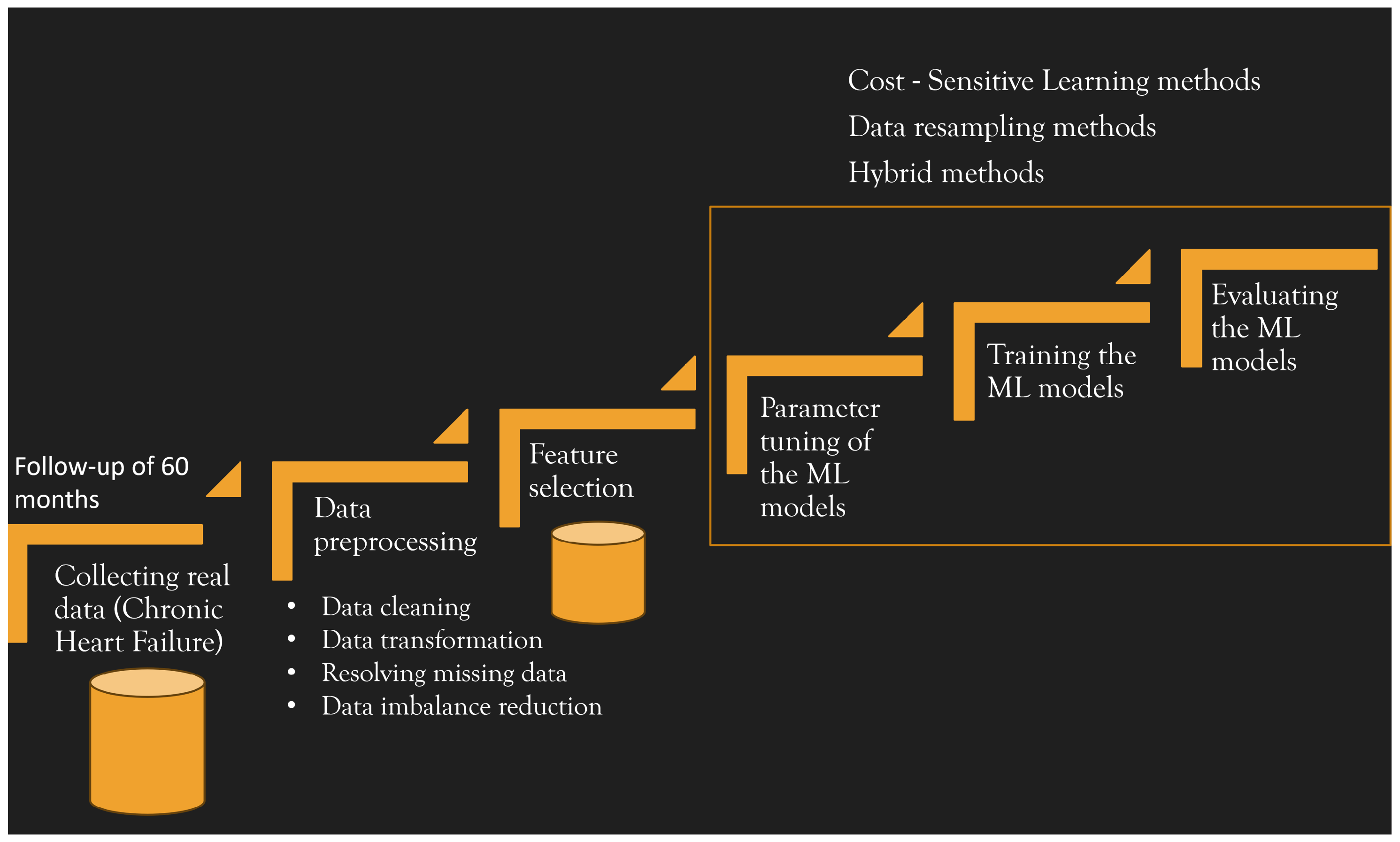
2. Real Data Collection and Dataset Construction

The data were collected over five years, as part of a pilot study conducted at the CHF outpatient clinic of the Geriatrics Division at the “Mater Domini” University Hospital in Catanzaro, Italy. The key steps undertaken are described below, and the statistical analysis was performed using R software, version 4.0.1 [33].

Study Population

A total of 154 patients suffering from CHF participated, comprising 119 men (77.3%) and 35 women (22.7%). However, only 50 patients (i.e., 32.5% of the total) who voluntarily provided their consent were enrolled in the pilot study. During the baseline assessment, all patients underwent medical history examination requiring a full physical examination. The medical history evaluation mainly focused on CV events, respiratory, and metabolic comorbidities, while key haemodynamic and anthropometric parameters were measured. The set of outpatients was meticulously monitored with a five-year follow-up conducted every 3 months. During each visit, six parameters were measured: weight, heart rate (HR), respiratory rate (RR), body temperature (BT), systolic blood pressure (SBP), and diastolic blood pressure (DBP). Clinical decompensation, with or without hospitalisation, and major CV events such as acute coronary syndrome, myocardial infarction, percutaneous transluminal coronary angioplasty (PTCA), surgical coronary artery revascularisation, stroke, death, and hospitalisation for any reason were reported. All clinical events had to be validated by source data (hospital records, death certificates or other original documents). Throughout the five-year follow-up, some patients missed a few medical visits, while others did not attend any appointments from the second-year onwards. Only eight patients completed the full five-year follow-up period.

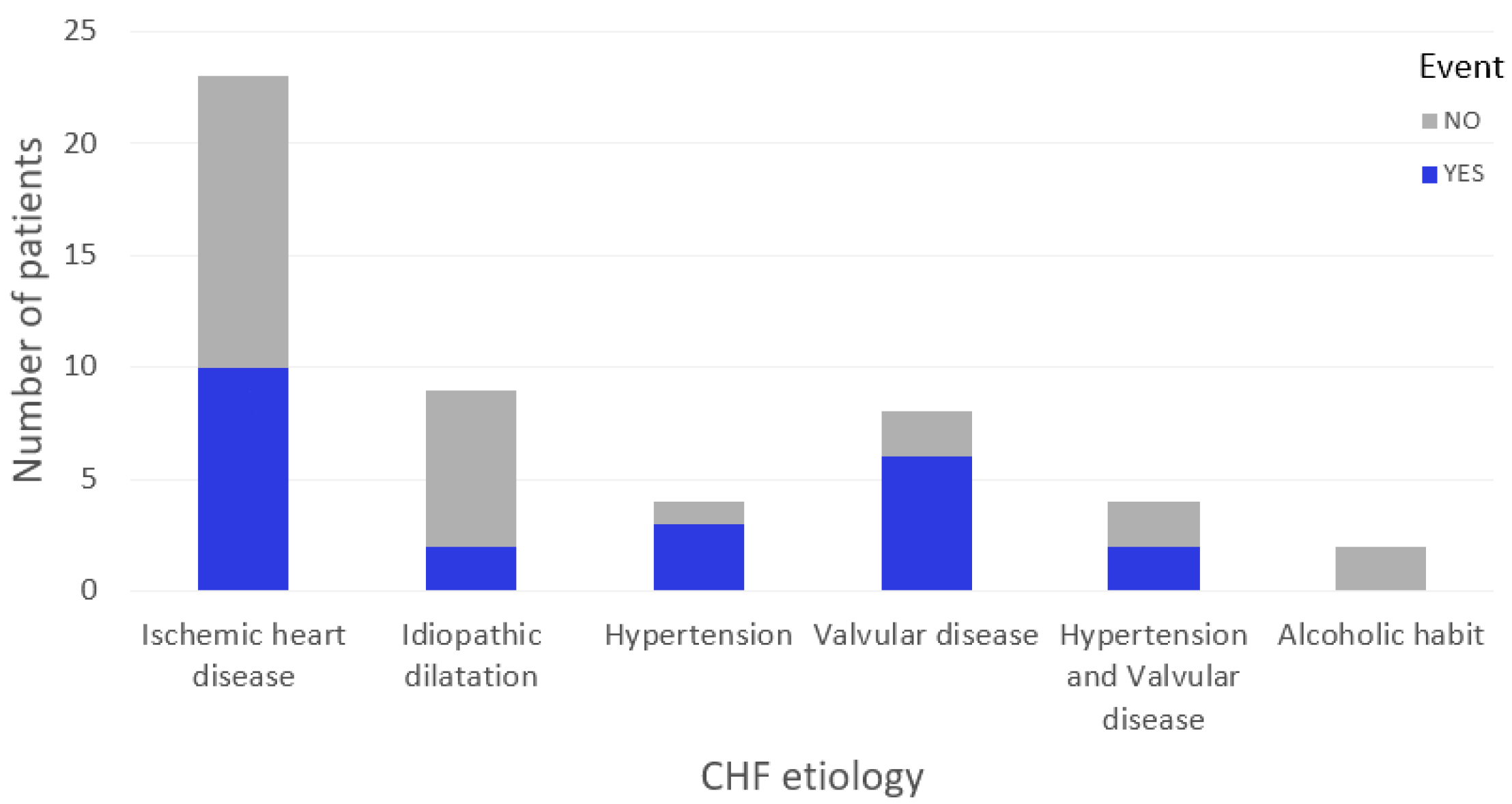
Patient Characteristics

Among the 50 enrolled patients, 14 were women (28%) and 36 were men (72%).

Table 1. Demographic and clinical characteristics of the patients. NYHA: New York Heart Association; CHF: chronic heart failure; PTCA: percutaneous transluminal coronary angioplasty; ICD: implantable cardioverter defibrillator; TIA: transient ischaemic attack; COPD: chronic obstructive pulmonary disease.

Characteristic
Age	(years ± SD)	72.5 ± 14.2
Sex	Male	36 (72%)
	Female	14 (28%)
NYHA Class	I	3 (6%)
	II	38 (76%)
	III	9 (18%)
CHF aetiology	Ischemic heart disease	23 (46%)
	Idiopathic dilatation	9 (18%)
	Hypertension	4 (8%)
	Valvular diseases	8 (16%)
	Valvular diseases + hypertension	4 (8%)
	Alcoholic habit	2 (4%)
Cardiovascular history	Instable angina	1 (2%)
	PTCA	1 (2%)
	By-pass	7 (14%)
	Atrial flutter	13 (26%)
	Pacemaker	3 (6%)
	Cardiac resynchronisation	1 (2%)
	ICD	2 (4%)
	Mitral insufficiency	21 (42%)
	Aortic insufficiency	4 (8%)
	Hypertension	28 (56%)
	TIA	2 (4%)
Other diseases	Diabetes	11 (22%)
	Hypothyroidism	1 (2%)
	Renal failure	4 (8%)
	COPD	5 (10%)
	Asthma	1 (2%)
	Sleep apnea	4 (8%)
	Pulmonary fibrosis	1 (2%)
	Gastrointestinal diseases	4 (8%)
	Hepatic diseases	3 (6%)
Pharmacological treatment	ACE-I/ARB	47 (94%)
	Diuretic therapy	29 (58%)
	Beta-blockers	44 (88%)
	Corticosteroids/NSAIDs	0 (0%)

summarises the demographic and clinical characteristics of the patients. The average age of the population was 72.5 ± 14.2 years. Among the patients, 3 (6%) showed a NYHA I class, 38 (76%) were in NYHA II class, and 9 (18%) in NYHA III class. The aetiology of CHF was represented as follows: ischaemic heart disease for 23 patients (46%); idiopathic dilated cardiomyopathy for 9 patients (18%); arterial hypertension for 4 patients (8%); valvular disease for 8 patients (16%); valvular disease that coexists with hypertension for 4 patients (8%); and alcoholic habit for 2 patients (4%). With regard to CV history, 1 patient (2%) had been revascularised by PTCA; 7 patients (14%) had undergone coronary artery bypass grafting; 13 patients (23%) had atrial flutter; 3 patients (6%) had undergone pacemaker implantation; 2 (4%) had implantable cardioverter defibrillator (ICD); 1 (2%) had undergone cardiac re-synchronisation therapy; 21 patients (42%) had mitral insufficiency; 4 patients (8%) had aortic insufficiency; 28 patients (56%) were hypertensive; and 2 patients (4%) suffered from a transitory ischaemic attack (TIA). In regard to the other comorbidities, 11 patients (22%) were diabetics, 1 patient (2%) had hypothyroidism, 4 patients (8%) suffered from chronic renal failure, 5 patients (10%) had chronic obstructive pulmonary disease (COPD), 1 patient (2%) suffered from bronchial asthma, 4 patients (8%) suffered from obstructive sleep apnoea, 4 patients (8%) suffered from gastrointestinal diseases and 3 patients (6%) suffered from liver disease. With regard to pharmacological treatment, 47 patients (94%) were on ACE-I/ARB, 29 patients (58%) were taking diuretic therapy, and 44 patients (88%) were receiving beta-blockers. No patients used corticosteroids or NSAIDs. Finally, 25 patients (50%) were taking triple therapy, 18 patients (36%) were receiving dual therapy with ACE-I/ARB - beta-blockers, 2 patients (4%) were on dual therapy with ACE-I/ARB and diuretic, whilst 5 patients (10%) were on single therapy.

Events during Follow-Up

During an average follow-up of 60 months, 19 patients presented a CV event. Among those patients who experienced an adverse event, 8 patients developed a second episode of decompensation. Notably, patients who manifested episodes of clinical instability were found to be older ($p<0.05$). Figure 2 displays the distribution of events based on the nine subtypes of CHF. Among the patients with ischaemic aetiology, 9 individuals (39.13%) had an event, while 2 patients (22.2%) were affected by idiopathic dilated cardiomyopathy; 2 patients (50%) had hypertensive aetiology; 3 patients (37.5%) had valvular disease; and 2 patients (50%) presented both valvular disease and hypertension. Interestingly, patients with alcoholic aetiology remained in stable clinical condition without any complications, in contrast to other types of CHF. Approximately half of the patients who experienced CV deterioration had a history of hypertension, and just under half had mitral insufficiency, while no patient with transient ischemic attack (TIA) presented further complications.

2.1. Data Preprocessing

A dataset consisting of 187 instances and suitable for the prediction task was created based on the collected data. Originally, the dataset was in a wide format with 50 rows, each containing personal data and a medical history of patients, along with visit dates, vital signs recorded at the visit, events occurring between the current and previous visits, and the corresponding event dates.

To perform the classification task, the data were converted into a long format where each row represents a patient’s visit. Input errors were corrected, outliers were discarded, and missing values were statistically imputed. Categorical variables with n values (e.g., aetiology, CV history, and other diseases) were converted into n numerical binary variables, while numerical data were expressed in their correct units of measurement. The resulting dataset comprises 794 instances and 37 features. Each instance was labelled as positive if there were CV deterioration events between two consecutive visits, and negative otherwise. Instances representing CV deterioration events were assigned to Class 1, while instances without any events were assigned to Class 2.

Imbalanced datasets are common in real-world applications and often become the focus of significant research efforts in knowledge discovery and data engineering. A dataset is considered imbalanced when one class, known as the minority class, is under-represented compared to the other class, which is the majority class. Relative imbalances frequently occur in practical scenarios, prompting extensive research in knowledge discovery and data engineering. For ML algorithms, imbalanced datasets pose a challenge because they tend to be overwhelmed by the abundance of majority class instances during the learning process. Therefore, methods are needed to improve recognition rates and address the issue of imbalanced data. In our dataset, the significant disparity between the number of negative instances (majority class) and positive instances (minority class) makes it imbalanced. Specifically, there are only 31 positive instances, accounting for a mere 4.6% of the entire dataset.

2.2. Feature Selection

Our aim was to develop a predictive model for the early detection of cardiovascular events in patients with CHF, utilising a limited set of basic clinical parameters. Through the feature selection process, vital signs were identified as the most informative factors. Vital signs, i.e., HR, RR, DPB, and SBP, were identified as the key factors for monitoring CHF and assessing the patient’s overall condition. These parameters play a crucial role in the predictive model’s design due to their significance in both CHF monitoring and patient assessment. Following the feature selection process, duplicate instances were removed from the dataset.

3. Machine Learning Process

In this section, we illustrate an overview of the entire machine learning process. We constructed, tested, and compared five ML predictive models, which are briefly introduced below. The details of this process are described in the subsequent section.

Supervised learning models were developed to accurately predict the risk of major events in CHF patients. The ML models implemented to develop the related prediction models are support vector machines (SVMs), artificial neural network, naïve Bayes, decision tree, and random forest.

SVM is based on the statistical learning theory [34,35] and is the most widely used ML technique available nowadays. It searches for an optimal hyperplane that separates the patterns of two classes by maximising the margin. Let X be a dataset with N instances $X=(x_1,\dots ,x_N)$, where $x_i,i=1,\dots ,N$, denotes an instance with m features, and $y_i\in \{\pm 1\}$ its label. Finding the optimal hyperplane means solving the quadratic programming model (1)–(3)

$$\begin{array}{cc}\hfill & min\frac{1}{2}{\left|\right|w\left|\right|}^2+C\sum _1^N{ϵ}_i\hfill \end{array}$$

(1)

$$\begin{array}{cc}\hfill & y_i(w^T\varphi \left(x_i\right)+b)-1+{ϵ}_i\ge 0i=1,\dots ,N\hfill \end{array}$$

(2)

$$\begin{array}{cc}\hfill & {ϵ}_i\ge 0i=1,\dots ,N\hfill \end{array}$$

(3)

where C, named penalty parameter, is a trade-off between the size of the margin and the slack variable penalty. In a non-linearly separable dataset, the SVM basically maps inputs into high-dimensional feature spaces by the so-called kernel functions. A kernel function denotes an inner product in a feature space, measures similarity between any pair of inputs $x_i$ and $x_j$, and is usually denoted by $K(x_i,x_j)=〈\varphi \left(x_i\right),\varphi \left(x_j\right)〉$ [36]. Here, we used three kernel functions: linear kernel $K(x_i,x_j)=〈x_i,x_j〉$, polynomial kernel $K(x_i,x_j)={(〈x_i,x_j〉+1)}^d$, and the RBF kernel $K(x_i,x_j)=exp(-\gamma ||x_i-x_j{\left|\right|}^2)$. The linear kernels are a special case of polynomial kernels as the degree d is set to 1 and they compute similarity in the input space, whereas the other kernel functions compute similarity in the feature space.

Artificial neural networks are computational models, consisting of a number of artificial neural units. They emulate biological neural networks [37]. In this study, we used a feed-forward artificial neural network named multilayer perceptron (MLP) with a three-layer structure of neurons: an input layer, one or more hidden layers with a variable number of neurons, and an output classification layer. The neurons in the MLP are trained with the back propagation learning algorithm [38].

Naïve Bayes [39] is a probabilistic ML algorithm based on the Bayes Theorem. It assumes that a particular feature in a class is unrelated to the presence of any other feature.

Decision trees are a non-parametric supervised learning method [40]. One of their main advantages is that they are simple to understand and interpret, and they can be visualised.

Random forest [41] consists of individual decision trees that operate as an ensemble. Each tree is built by applying bagging, which is the general technique of bootstrap aggregation. A simple majority vote of all trees gives the final result. RF had good accuracy results in medical diagnosis problems [42,43].

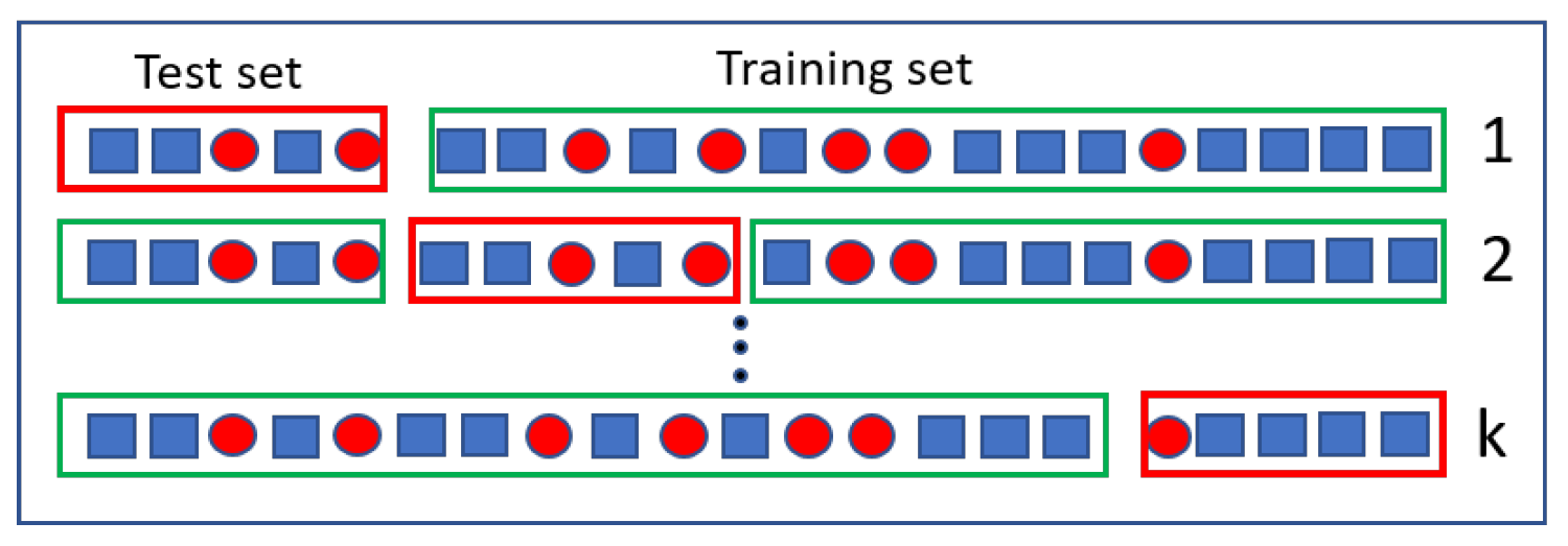
3.1. Dealing with Imbalance Data: Cost-Sensitive Learning and Methods for Model Assessment

The problem addressed here is one of the most challenging issues in applied ML, as the event cases are under-represented. It is strongly important to correctly identify instances from the minority class compared to the majority class. To handle this problem, specific methods need to be employed. Usually, misclassification errors are treated equally but they are different depending on the class. In this work, we use and test cost-sensitive algorithms which involve the use of different misclassification costs.

A general cost matrix $Cost$ denotes the cost of each class misclassification [44]. A cost matrix for datasets with two classes is illustrated in

Table 2. Cost matrix for a binary classification problem.

		Actual Class
		Positive	Negative
Predicted class	Positive	$c_{11}$	$c_{12}$
	Negative	$c_{21}$	$c_{22}$

.

In general, $c_{ij}$ is the cost of predicting an instance belonging to class i as belonging to class j. The goal of this type of learning is to minimise the total misclassification cost of a model on the training set. Formally, given a cost matrix $Cost$ and an instance x, the cost $R\left(i\right|x)$ of classifying x into class i is $R\left(i\right|x)={\sum }_{j}p\left(j\right|x)c_{ij}$, where $p\left(j\right|x)$ is the probability estimation of classifying an instance into class j. In the above cost matrix, $c_{12}$ represents the cost of a false positive misclassification and $c_{21}$ is the cost of a false negative misclassification. Usually, as we also assume here, there is no cost for correct classifications, that is, $c_{11}=c_{22}=0$. We tested different cost matrices, as detailed in the next section.

3.2. Hybrid Method for Imbalanced Dataset and Hyper-Parameter Optimisation Approach

Our dataset suffers from class imbalance, a common issue wherein classifiers developed on such data tend to be biased towards negative predictions due to the majority class having no-event cases. To address this problem and enable the better generalisation to new data, it is essential to use appropriate methods for handling imbalanced classes. The main methods for sampling-based imbalance correction are based on over-sampling and under-sampling. Over-sampling methods involves adding more data to the smaller class equalising its size with the larger class. On the other hand, under-sampling methods involve randomly selecting data from the larger class, matching its size with the smaller class. To tackle the class imbalance in our study, we adopted a hybrid method that balances the class distribution by combining over-sampling and under-sampling approaches. This approach adds data in the minority class while simultaneously removing data from the majority class, achieving a more balanced representation of both classes in the dataset.

To assess the models, we conducted a k-fold cross-validation process, ensuring the use of k independent sets to test the model, effectively simulating unseen data. The procedure basically consists in randomly partitioning the dataset into k equal-sized folds. During each of the k rounds, the $k$-th fold is the test set while the remaining folds are used as the training set. The test set is never used during the training of the model, preventing overfitting. Each fold is used exactly once as a test set, ensuring that each instance is used for testing exactly once. Figure 3 provides a schematic representation of the k-fold cross-validation process. The performance metrics are averaged across the k estimates from each test fold. In a well-designed k-fold cross-validation procedure, it is crucial to determine the training and test partitions before applying any oversampling technique. As thoroughly discussed in [45], conducting k-fold cross-validation on imbalanced data could have overly optimistic estimates if oversampling methods are applied to the entire dataset. To ensure a reliable evaluation of the model’s ability to generalise to real-world data, the oversampling should only be applied to the folds designated as training data. This approach maintains the integrity of the test sets, providing a more accurate assessment of the model’s performance.

The impact of hyper-parameters on the performance of an ML model is widely recognised. Generally, the hyper-parameters of each model are adjusted to find a hyper-parameter setting that maximises the model performances and enables accurate predictions on unseen data. Recent studies proved that hyper-parameter tuning with class weight optimisation are efficient in handling imbalanced data [46,47,48,49,50]. In this study, we employed the grid search optimisation strategy [51] to determine the optimal hyper-parameters for each ML model on the entire dataset. This strategy involves exploring all specified hyper-parameter combinations within a multi-dimensional grid. Each combination is evaluated using a performance metric to assess its effectiveness in enhancing the model’s performance. Multiple combinations of hyper-parameters are evaluated during the Grid Search optimisation process. Among these combinations, the one that yields the best performance is selected. Subsequently, this optimal set of hyper-parameters is utilised to train the ML model on the entire dataset.

3.3. Performance Metrics for Imbalanced Dataset

The predictive performance of the constructed ML models is evaluated and compared using various metrics, including the receiver operating characteristic (ROC—area under the curve (AUC), sensitivity, specificity, balanced accuracy, and G-mean values.

Let P and N be the numbers of positive and negative instances in the dataset, respectively. Let $TP$ and $TN$ be the numbers of instances correctly predicted as positive and negative, respectively, and $FP$ and $FN$ be the number of instances predicted as positive and negative while actually belonging to the opposite class, respectively.

• AUC measures the classifier’s ability to avoid false classification [52]. It is the area under the curve of the true positive ratio vs. the false positive ratio that indicates the probability that the model will rank a positive case more highly than a negative case. A model whose predictions are 100% correct has an AUC of 1.0.
• Sensitivity, also referred to as true positive rate or recall, measures the proportion of positive instances that are correctly identified, i.e., it is the ability to predict a CV event:

  $$\begin{array}{c}\hfill \mathrm{Sens}=\frac{TP}{TP+FN}\end{array}$$
• Specificity (also known as true negative rate) is used to determine the ability to correctly classify. It measures the proportion of negatives that are correctly identified, and is defined as

  $$\begin{array}{c}\hfill \mathrm{Spec}=\frac{TN}{TN+FP}\end{array}$$
• The accuracy metric can be misleading for our imbalanced dataset. As it is equally important to accurately predict the events of the positive and negative classes for the addressed problem, we used the balanced accuracy metric [53,54], which is defined as the arithmetic mean of sensitivity and specificity:

  $$\begin{array}{c}\hfill \mathrm{B-acc}={\displaystyle \frac{\mathrm{Sens}+\mathrm{Spec}}{2}}=\frac{TPR+TNR}{2}\end{array}$$
• Another useful metric is the so-called geometric mean or G-Mean that balances both sensitivity and specificity by combining them. It is defined as

  $$\begin{array}{c}\hfill \mathrm{G-Mean}=sqrt(Sens\ast Spec)\end{array}$$

The sensitivity and specificity are also known as quality parameters and used to define the quality of the predicted class.

4. Results and Discussions

For predicting cardiovascular deterioration events in CHF patients, we only used the vital signs as predictive features for a deterioration event. With the aim of finding an ML model that is able to predict CV events, we carried out computational experiments with three methods, named as follows:

• Method₁: cost-sensitive learning methods;
• Method₂: data resampling methods;
• Method₃: cost-sensitive learning methods combined with data resampling methods.

In cost-sensitive learning, we considered the cost of misclassifying a positive instance and the cost of misclassifying a negative instance as hyper-parameters to be tuned during the model training process. Referring to the notation of Table 2, we fixed the misclassification cost $c_{12}=1$ and explored different values for

$c_{21}\in \{1,1.5,2,5,10,20,30,40,50,100,200,300,400\}$, while setting $c_{11}=c_{22}=0$.

The Waikato Environment for Knowledge Analysis (Weka, version 3.8.2, [55]) was utilised for constructing and evaluating the classification models. For each ML model, we used the grid search algorithm to select the optimal values of the cost matrix.

Table 3. Hyper-parameter tuning for SVM and MLP and best values.

ML Model	Parameter	Search Space	Step	Selected Value
SVM	d	[1, 5]	1	2
(polynomial kernel)	C	[1, 10]	0.5	5
SVM	$\gamma$	[0.01, 1.00]	0.01	0.82
(RBF kernel)	C	[1, 10]	0.5	3
MLP	Learning rate	[0.1, 1.0]	0.1	0.6
	Momentum	[0.1, 1.0]	0.1	0.1
	Number of epochs	[400, 600]	100	500

presents the hyper-parameter tuning performed with a data resampling approach for SVM and MLP. The final column displays the optimal hyper-parameter values, as follows:

 SVM: 

We tested SVM with three kernel functions, i.e., the linear kernel, polynomial kernel, and RBF kernel. The hyper-parameter C and those related to the polynomial kernel and RBF kernel were optimised by searching for the best values within the specified range, as reported in Table 3. The incremental value used for optimisation is denoted in the fourth column as “Step.”

 MLP: 

The model parameter optimisation involves choosing the number of hidden layers, the number of neurons in each layer, the number of epochs, the learning rate, and the momentum. We tested different MLP models consisting of one input layer, one output layer, and one hidden layer. The number of neurons in the hidden layer was set according to the formula

$$\begin{array}{c}\hfill nr.neurons={\displaystyle \frac{nr.ofinputfeatures+nr.ofclasses}{2}}\end{array}$$

We optimised the learning rate, the momentum, and the number of epochs in a defined range of values, as reported in Table 3. The incremented value is denoted in the fourth column as “Step”.

Table 3 presents the values tested for optimising the hyper-parameters of SVM and MLP models through the grid search algorithm. The results of the hyper-parameter tuning for both SVM and MLP models using a cost matrix with equal misclassification costs (i.e., false negative cost and false positive cost) are shown as optimal hyper-parameter values in the last column.

Table 4. Optimal hyper-parameters values.

Model	Parameter	Value
SVM with linear kernel	C	1
SVM with polynomial kernel	d	2
	C	5
SVM with RBF kernel	$\gamma$	0.82
	C	3
MLP	Learning rate	0.6
	Momentum	0.1
	Number of epochs	500
	Number of neurons in input layer	4
	Number of neurons in hidden layer	3
	Number of neurons in output layer	2
Naive Bayes	useKernelEstimator	False
	useSupervisedDiscretisation	False
Decision tree	Confidence factor	0.25
Random forest	Bag size percent	100
	Number of iterations	100

displays the hyper-parameter values set for each model, alongside the corresponding cost matrix with equal misclassification costs. The table provides a comprehensive overview of the selected hyper-parameter values for each model in the study and the same cost matrix.

Predictive Models Performance Metrics

We carried out computational experiments with the three methods. The following tables only report the best performance results. The performance metrics are related to both three-fold cross-validation and five-fold cross-validation. The best values for each performance metric achieved by a ML model are highlighted in bold.

Table 5. Predictive cost-sensitive learning model performance metrics by the cost-sensitive method.

			3-Fold Cross-Validation					5-Fold Cross-Validation
Model	c12	c21	AUC	Sens	Spec	B-acc	G-mean	AUC	Sens	Spec	B-acc	G-mean
SVM with linear kernel	1	10	0.535	0.130	0.940	0.536	0.278	0.611	0.257	0.964	0.611	0.498
	1	20	0.597	0.394	0.801	0.598	0.542	0.703	0.586	0.820	0.703	0.693
	1	30	0.576	0.558	0.594	0.576	0.557	0.670	0.719	0.620	0.670	0.668
	1	35	0.499	0.621	0.376	0.499	0.429	0.601	0.752	0.449	0.601	0.581
	1	40	0.482	0.788	0.176	0.482	0.182	0.535	0.881	0.189	0.535	0.408
SVM with polynomial kernel	1	10	0.542	0.13	0.954	0.542	0.278	0.583	0.195	0.972	0.584	0.435
	1	20	0.609	0.33	0.889	0.610	0.515	0.635	0.357	0.913	0.635	0.571
	1	30	0.544	0.397	0.692	0.545	0.488	0.586	0.843	0.329	0.586	0.527
	1	35	0.544	0.745	0.341	0.544	0.485	0.565	0.719	0.412	0.566	0.544
	1	40	0.472	0.621	0.322	0.472	0.414	0.544	0.786	0.303	0.545	0.488
SVM with RBF kernel	1	10	0.557	0.161	0.952	0.557	0.317	0.583	0.19	0.976	0.583	0.431
	1	20	0.546	0.227	0.865	0.546	0.428	0.661	0.424	0.898	0.661	0.617
	1	30	0.578	0.558	0.599	0.579	0.559	0.677	0.719	0.635	0.677	0.676
	1	35	0.551	0.555	0.548	0.552	0.534	0.589	0.69	0.487	0.589	0.580
	1	40	0.505	0.558	0.452	0.505	0.470	0.548	0.724	0.371	0.548	0.518
MLP	1	10	0.579	0.464	0.641	0.553	0.279	0.72	0.362	0.83	0.596	0.548
	1	15	0.528	0.464	0.652	0.558	0.280	0.716	0.633	0.382	0.508	0.492
	1	20	0.609	1.000	0.000	0.500	0.000	0.559	1.000	0.000	0.500	0.000
Naive Bayes	1	10	0.619	0.324	0.886	0.606	0.528	0.667	0.257	0.91	0.584	0.484
	1	20	0.619	0.391	0.807	0.599	0.555	0.667	0.390	0.826	0.608	0.568
	1	30	0.619	0.455	0.724	0.590	0.565	0.667	0.490	0.746	0.618	0.605
	1	40	0.619	0.485	0.621	0.553	0.539	0.667	0.586	0.655	0.621	0.620
	1	50	0.619	0.518	0.510	0.515	0.509	0.667	0.619	0.562	0.591	0.590
	1	60	0.619	0.615	0.448	0.532	0.519	-	-	-	-	-
Decision tree	1	10	0.553	0.197	0.916	0.557	0.412	0.526	0.133	0.921	0.527	0.35
	1	20	0.56	0.197	0.924	0.561	0.415	0.527	0.133	0.919	0.526	0.350
	1	30	0.563	0.230	0.898	0.564	0.434	0.553	0.200	0.897	0.549	0.424
	1	40	0.533	0.197	0.870	0.534	0.402	0.568	0.233	0.892	0.563	0.456
	1	50	0.543	0.230	0.863	0.547	0.425	0.577	0.267	0.874	0.571	0.483
	1	100	0.572	0.364	0.773	0.568	0.477	0.578	0.324	0.805	0.565	0.511
	1	200	0.554	0.430	0.672	0.551	0.484	0.618	0.590	0.611	0.601	0.600
	1	300	0.538	0.524	0.515	0.520	0.496	0.642	0.652	0.473	0.563	0.555
	1	350	0.516	0.691	0.296	0.493	0.292	-	-	-	-	-
	1	400	0.516	0.691	0.296	0.493	0.292	-	-	-	-	-
Random forest	1	10	0.593	0.164	0.961	0.563	0.380	0.639	0.100	0.972	0.536	0.312
	1	20	0.579	0.164	0.961	0.563	0.380	0.617	0.100	0.964	0.532	0.310
	1	30	0.596	0.164	0.958	0.561	0.379	0.618	0.200	0.958	0.579	0.438
	1	40	0.585	0.197	0.954	0.576	0.405	0.626	0.167	0.957	0.562	0.400
	1	50	0.572	0.197	0.952	0.575	0.405	0.624	0.200	0.949	0.575	0.436
	1	100	0.587	0.164	0.929	0.547	0.374	0.629	0.262	0.930	0.596	0.494
	1	200	0.595	0.230	0.879	0.555	0.413	0.601	0.324	0.865	0.595	0.529
	1	300	0.568	0.364	0.787	0.576	0.496	0.597	0.390	0.759	0.575	0.544
	1	400	0.568	0.330	0.684	0.508	0.429	0.599	0.486	0.690	0.588	0.579
	1	500	0.562	0.397	0.610	0.508	0.429	0.588	0.552	0.602	0.577	0.576

summarises the best results related to $Metho{d}_1$, i.e., cost-sensitive learning methods. The SVM models with the linear kernel and RBF kernel demonstrated the best overall performances compared to the other models when the misclassification costs were set to $c_{12}=1$ and $c_{21}=30$. The decision tree models exhibited a comparable prediction performance in terms of sensitivity and specificity only when the cost of misclassifying the minority class was set to a high value, that is, $c_{21}=200$ or $c_{21}=300$. Naive Bayes models showed a comparable prediction performance with both $c_{21}=30$ and $c_{21}=40$ with five-fold cross-validation. Random forest models showed a comparable prediction performance only when the cost of misclassifying the minority class was set to a high value, that is, $c_{21}=500$. Furthermore, it is noteworthy that, in general, hyper-parameters that allow one to find the highest sensitivity have the lowest specificity, and vice versa.

Table 6. Predictive model performance metrics related to the data resampling method, and the cost-sensitive method combined with the data resampling method.

			3-Fold Cross-Validation					5-Fold Cross-Validation
Model	c12	c21	AUC	Sens	Spec	B-acc	G-mean	AUC	Sens	Spec	B-acc	G-mean
SVM with linear kernel	1	1	0.573	0.394	0.752	0.573	0.522	0.680	0.557	0.802	0.680	0.668
	1	1.5	0.522	0.527	0.517	0.573	0.522	0.670	0.781	0.560	0.671	0.661
	1	2	0.459	0.685	0.232	0.459	0.279	0.545	0.876	0.214	0.545	0.433
	1	5	0.500	1.000	0.000	0.500	0.000	0.500	1.000	0.000	0.500	0.000
SVM with polynomial kernel	1	1	0.536	0.355	0.717	0.536	0.498	0.578	0.324	0.832	0.578	0.519
	1	1.5	0.569	0.812	0.325	0.536	0.498	0.577	0.843	0.310	0.577	0.511
	1	2	0.541	0.812	0.271	0.542	0.447	0.520	0.814	0.226	0.520	0.429
	1	5	0.515	0.842	0.187	0.515	0.374	0.471	0.843	0.099	0.471	0.289
	1	10	0.476	0.936	0.017	0.477	0.099	0.505	1.000	0.009	0.505	0.095
	1	20	0.500	1.000	0.000	0.500	0.000	0.500	1.000	0.000	0.500	0.000
	1	30	0.473	0.906	0.041	0.474	0.145	0.503	1.000	0.006	0.503	0.077
SVM with RBF kernel	1	1	0.596	0.427	0.763	0.596	0.550	0.644	0.452	0.835	0.644	0.614
	1	1.5	0.519	0.458	0.580	0.596	0.550	0.638	0.657	0.619	0.638	0.638
	1	2	0.521	0.558	0.484	0.521	0.480	0.586	0.748	0.425	0.587	0.564
	1	5	0.466	0.812	0.120	0.466	0.234	0.465	0.876	0.054	0.465	0.218
	1	10	0.500	1.000	0.000	0.500	0.000	0.500	1.000	0.000	0.500	0.000
MLP	1	1	0.634	0.397	0.680	0.538	0.475	0.659	0.557	0.764	0.661	0.652
	1	2	0.606	0.697	0.293	0.495	0.094	0.715	0.652	0.555	0.604	0.602
	1	5	0.598	0.652	0.574	0.613	0.591	0.695	0.781	0.396	0.589	0.556
	1	10	0.548	0.767	0.351	0.559	0.385	0.663	0.724	0.348	0.536	0.502
	1	20	0.498	0.652	0.385	0.519	0.446	0.629	0.790	0.136	0.463	0.328
	1	30	0.533	0.632	0.416	0.524	0.500	0.570	0.752	0.180	0.466	0.368
Naive Bayes	1	1	0.619	0.391	0.789	0.590	0.548	0.680	0.424	0.797	0.611	0.581
	1	1.5	0.619	0.488	0.681	0.590	0.548	0.680	0.552	0.716	0.634	0.629
	1	2	0.619	0.548	0.588	0.569	0.560	0.680	0.619	0.607	0.613	0.613
	1	5	0.619	0.879	0.201	0.540	0.388	0.680	0.843	0.202	0.523	0.413
	1	10	0.619	0.879	0.093	0.486	0.170	0.680	0.910	0.0434	0.477	0.199
	1	20	0.619	0.939	0.057	0.498	0.125	0.680	1.000	0.012	0.506	0.110
	1	30	0.619	0.939	0.039	0.489	0.103	0.680	1.000	0.006	0.503	0.078
Decision tree	1	1	0.524	0.164	0.884	0.524	0.293	0.617	0.357	0.864	0.611	0.555
	1	2	0.540	0.197	0.874	0.536	0.389	0.602	0.324	0.871	0.598	0.531
	1	5	0.515	0.297	0.754	0.526	0.445	0.615	0.457	0.741	0.599	0.582
	1	10	0.500	0.464	0.520	0.492	0.418	0.621	0.586	0.618	0.602	0.602
	1	20	0.509	0.555	0.430	0.493	0.460	0.613	0.648	0.448	0.548	0.539
	1	30	0.475	0.621	0.339	0.480	0.304	0.473	0.748	0.155	0.452	0.340
Random forest	1	1	0.595	0.164	0.921	0.542	0.372	0.640	0.195	0.931	0.563	0.426
	1	2	0.570	0.230	0.916	0.573	0.422	0.638	0.257	0.933	0.595	0.490
	1	5	0.599	0.230	0.879	0.555	0.431	0.638	0.257	0.895	0.576	0.480
	1	10	0.580	0.330	0.807	0.569	0.485	0.613	0.390	0.828	0.609	0.568
	1	20	0.568	0.430	0.630	0.531	0.473	0.634	0.552	0.675	0.614	0.610
	1	30	0.572	0.558	0.505	0.531	0.500	0.601	0.619	0.503	0.561	0.558

reports the performance of the predictive models with $Metho{d}_2$ and $Metho{d}_3$. More specifically, the first row shows the results found by $Metho{d}_2$ per each ML model reported in the first columns; the rest of the rows show the results found by $Metho{d}_3$. Based on the performance results, the MLP with $c_{12}=1,c_{21}=2$ has the best performance among the built models with a mean sensitivity and a mean specificity of 65% and 55%, respectively, a mean area under the curve of 0.71, and a G-mean of 0.60. In general, we observed that the performance of the predictive models MLP, naive Bayes, decision tree, and random forest improved when the cost of misclassifying the minority class was higher ($c_{21}>c_{12}$). Additionally, all constructed models achieved a meaningful prediction performance with a five-fold cross-validation approach. However, the SVM model with a polynomial kernel showed a lower sensitivity performance in certain cases. These findings indicate that the combination of cost-sensitive methods with data over/under-sampling approaches is effective for the meaningful prediction of cardiovascular events. Comparing the three methods, the cost-sensitive learning methods proved to be superior to the sampling approach. They achieved a high performance in terms of G-mean, indicating their efficacy in handling imbalanced data and improving the model’s overall performance.

This model could be particularly useful in CHF patients with NYHA class III or IV, where functional reserves are reduced and each exacerbation leads to a further deterioration of cardiac function that worsens the symptomatology and often requires hospitalisation and sometimes results in death. In this context, the early identification and treatment of a re-exacerbation of HF may improve the patient’s symptoms and prognosis and avoid hospitalisation with reduced healthcare costs [6].

5. Conclusions

Technology is increasingly playing a significant role in clinical practice. In this context, machine learning represents an innovative methodology for managing chronic disorders, empowering clinicians with a key role in predicting cardiovascular events rather than merely being spectators.

The data used in this study were collected during a pilot study in a well-characterised CHF population of patients. The results open up numerous potential perspectives for applying ML approaches to clinical practice. Having a predictive system for CV deterioration events in CHF patients can lead to significant advantages, such as reducing hospitalisations and associated costs. The clinical importance of utilising such a model cannot be understated, as early detection can prevent CV events, improve patient health, and optimise healthcare expenditure.

The findings suggest that cost-sensitive methods can effectively predict CV deterioration events in CHF patients using only a few clinical variables. CHF remains one of the most severe chronic diseases in terms of mortality, hospitalisation rate, and healthcare costs. Successfully addressing even one variable linked to the natural course of this disease would be a significant achievement, benefiting the patients, clinicians, and the National Health System. Our KD process yielded promising results, paving the way for large-scale application. It is interesting that a few clinical variables such as HR, RR, DBP, and SBP had a good performance in the prediction of CV deterioration events. Furthermore, the performance of these models may be enhanced by including other variables of study patients. Further studies, however, are needed to validate this approach in a more large-scaled patient population. As part of future work, we plan to expand the sample size by including more patients, reducing the interval between consecutive visits using remote monitoring, and conduct an in-depth feature selection study to better understand which other features are crucial in diagnosing deterioration events in CHF patients.

References

1. Disease and Injury Incidence and Prevalence Collaborators. Global, regional, and national incidence, prevalence, and years lived with disability for 354 diseases and injuries for 195 countries and territories, 1990–2017: A systematic analysis for the Global Burden of Disease Study 2017. Lancet 2018, 392, 1789–1858. [Google Scholar] [CrossRef] [PubMed]
2. McMurray, J.J. Improving outcomes in heart failure: A personal perspective. Eur. Heart J. 2015, 36, 3467–3470. [Google Scholar] [CrossRef] [PubMed]
3. Wang, T.; Evans, J.C.; Benjamin, E.; Lévy, D.; Leroy, E.; Vasan, R. Natural History of Asymptomatic Left Ventricular Systolic Dysfunction in the Community. Circ. J. Am. Heart Assoc. 2003, 108, 977–982. [Google Scholar] [CrossRef] [PubMed]
4. Dunlay, S.M.; Redfield, M.M.; Weston, S.A.; Therneau, T.M.; Long, K.H.; Shah, N.D.; Roger, V.L. Hospitalizations after Heart Failure Diagnosis. J. Am. Coll. Cardiol. 2009, 54, 1695–1702. [Google Scholar] [CrossRef]
5. Ponikowski, P.; Voors, A.A.; Anker, S.D.; Bueno, H.; Cleland, J.G.F.; Coats, A.J.S.; Falk, V.; González-Juanatey, J.R.; Harjola, V.P.; Jankowska, E.A.; et al. 2016 ESC Guidelines for the diagnosis and treatment of acute and chronic heart failure: The Task Force for the diagnosis and treatment of acute and chronic heart failure of the European Society of Cardiology (ESC)Developed with the special contribution of the Heart Failure Association (HFA) of the ESC. Eur. Heart J. 2016, 37, 2129–2200. [Google Scholar] [CrossRef]
6. McDonagh, T.A.; Metra, M.; Adamo, M.; Gardner, R.S.; Baumbach, A.; Bohm, M.; Burri, H.; Butler, J.; Celutkien, J.; Chioncel, O.; et al. 2021 ESC Guidelines for the diagnosis and treatment of acute and chronic heart failure: Developed by the Task Force for the diagnosis and treatment of acute and chronic heart failure of the European Society of Cardiology (ESC) With the special contribution of the Heart Failure Association (HFA) of the ESC. Eur. Heart J. 2021, 42, 3599–3726. [Google Scholar]
7. Stevenson, L.W.; Pagani, F.D.; Young, J.B.; Jessup, M.; Miller, L.; Kormos, R.L.; Naftel, D.C.; Ulisney, K.; Desvigne-Nickens, P.; Kirklin, J.K. INTERMACS profiles of advanced heart failure: The current picture. J. Heart Lung Transplant. Off. Publ. Int. Soc. Heart Transplant. 2009, 28, 535–541. [Google Scholar] [CrossRef]
8. Ziaeian, B.; Fonarow, G. Epidemiology and aetiology of heart failure. Nat. Rev. Cardiol. 2016, 13, 368–378. [Google Scholar] [CrossRef]
9. Mehta, P.A.; Dubrey, S.W.; McIntyre, H.F.; Walker, D.M.; Hardman, S.M.C.; Sutton, G.C.; McDonagh, T.A.; Cowie, M.R. Improving survival in the 6 months after diagnosis of heart failure in the past decade: Population-based data from the UK. Heart 2009, 95, 1851–1856. [Google Scholar] [CrossRef]
10. Tavazzi, L.; Senni, M.; Metra, M.; Gorini, M.; Cacciatore, G.; Chinaglia, A.; Lenarda, A.D.; Mortara, A.; Oliva, F.; Maggioni, A.P. Multicenter Prospective Observational Study on Acute and Chronic Heart Failure. Circ. Heart Fail. 2013, 6, 473–481. [Google Scholar] [CrossRef]
11. Liao, L.; Allen, L.A.; Whellan, D.J. Economic burden of heart failure in the elderly. PharmacoEconomics 2008, 26, 447–462. [Google Scholar] [CrossRef]
12. Stewart, S.; Jenkins, A.; Buchan, S.; McGuire, A.; Capewell, S.; McMurray, J. The current cost of heart failure to the National Health Service in the UK. Eur. J. Heart Fail. 2002, 4, 361–371. [Google Scholar] [CrossRef] [PubMed]
13. Marangoni, E.; Lissoni, F.; Raimondi Cominesi, I.; Tinelli, S. Heart failure: Epidemiology, costs and healthcare programs in Italy. G. Ital. Cardiol. 2012, 13, 139S–144S. [Google Scholar] [CrossRef]
14. Krumholz, H.M.; Chen, Y.T.; Vaccarino, V.; Wang, Y.; Radford, M.J.; Bradford, W.; Horwitz, R.I. Correlates and impact on outcomes of worsening renal function in patients ≥ years of age with heart failure. Am. J. Cardiol. 2000, 85, 1110–1113. [Google Scholar] [CrossRef] [PubMed]
15. Brons, M.; Koudstaal, S.; Asselbergs, F.W. Algorithms used in telemonitoring programmes for patients with chronic heart failure: A systematic review. Eur. J. Cardiovasc. Nurs. 2018, 17, 580–588. [Google Scholar] [CrossRef]
16. Kurtz, B.; Lemercier, M.; Pouchin, S.C.; Benmokhtar, E.; Vallet, C.; Cribier, A.; Bauer, F. Automated home telephone self-monitoring reduces hospitalization in patients with advanced heart failure. J. Telemed. Telecare 2011, 17, 298–302. [Google Scholar] [CrossRef]
17. Olsen, C.R.; Mentz, R.J.; Anstrom, K.J.; Page, D.; Patel, P.A. Clinical applications of machine learning in the diagnosis, classification, and prediction of heart failure. Am. Heart J. 2020, 229, 1–17. [Google Scholar] [CrossRef] [PubMed]
18. Averbuch, T.; Sullivan, K.; Sauer, A.; Mamas, M.A.; Voors, A.A.; Gale, C.P.; Metra, M.; Ravindra, N.; Van Spall, H.G.C. Applications of artificial intelligence and machine learning in heart failure. Eur. Heart J.-Digit. Health 2022, 3, 311–322. [Google Scholar] [CrossRef] [PubMed]
19. Lofaro, D.; Groccia, M.C.; Guido, R.; Conforti, D.; Caroleo, S.; Fragomeni, G. Machine learning approaches for supporting patient-specific cardiac rehabilitation programs. In Proceedings of the 2016 Computing in Cardiology Conference (CinC), Vancouver, BC, Canada, 11–14 September 2016; pp. 149–152. [Google Scholar]
20. Groccia, M.C.; Lofaro, D.; Guido, R.; Conforti, D.; Sciacqua, A. Predictive Models for Risk Assessment of Worsening Events in Chronic Heart Failure Patients. In Proceedings of the 2018 Computing in Cardiology Conference (CinC), Maastricht, The Netherlands, 23–26 September 2018; Volume 45, pp. 1–4. [Google Scholar] [CrossRef]
21. Tripoliti, E.E.; Papadopoulos, T.G.; Karanasiou, G.S.; Naka, K.K.; Fotiadis, D.I. Heart failure: Diagnosis, severity estimation and prediction of adverse events through machine learning techniques. Comput. Struct. Biotechnol. J. 2017, 15, 26–47. [Google Scholar] [CrossRef]
22. Lorenzoni, G.; Sabato, S.S.; Lanera, C.; Bottigliengo, D.; Minto, C.; Ocagli, H.; De Paolis, P.; Gregori, D.; Iliceto, S.; Pisanò, F. Comparison of machine learning techniques for prediction of hospitalization in heart failure patients. J. Clin. Med. 2019, 8, 1298. [Google Scholar] [CrossRef]
23. Lemaître, G.; Nogueira, F.; Aridas, C.K. Imbalanced-learn: A python toolbox to tackle the curse of imbalanced datasets in machine learning. J. Mach. Learn. Res. 2017, 18, 559–563. [Google Scholar]
24. Chawla, N.V.; Bowyer, K.W.; Hall, L.O.; Kegelmeyer, W.P. SMOTE: Synthetic minority over-sampling technique. J. Artif. Intell. Res. 2002, 16, 321–357. [Google Scholar] [CrossRef]
25. Beckmann, M.; Ebecken, N.F.; de Lima, B.S.P. A KNN undersampling approach for data balancing. J. Intell. Learn. Syst. Appl. 2015, 7, 104. [Google Scholar] [CrossRef]
26. Akbani, R.; Kwek, S.; Japkowicz, N. Applying support vector machines to imbalanced datasets. In Proceedings of the European Conference on Machine Learning, Pisa, Italy, 20–24 September 2004; Springer: Berlin/Heidelberg, Germany, 2004; pp. 39–50. [Google Scholar]
27. Cheng, F.; Zhang, J.; Wen, C. Cost-sensitive large margin distribution machine for classification of imbalanced data. Pattern Recognit. Lett. 2016, 80, 107–112. [Google Scholar] [CrossRef]
28. Veropoulos, K.; Campbell, C.; Cristianini, N. Controlling the sensitivity of support vector machines. In Proceedings of the International Joint Conference on AI, Stockholm, Sweden, 31 July–6 August 1999; Volume 55, p. 60. [Google Scholar]
29. Qi, Z.; Tian, Y.; Shi, Y.; Yu, X. Cost-sensitive support vector machine for semi-supervised learning. Procedia Comput. Sci. 2013, 18, 1684–1689. [Google Scholar] [CrossRef]
30. Tao, X.; Li, Q.; Guo, W.; Ren, C.; Li, C.; Liu, R.; Zou, J. Self-adaptive cost weights-based support vector machine cost-sensitive ensemble for imbalanced data classification. Inf. Sci. 2019, 487, 31–56. [Google Scholar] [CrossRef]
31. Thai-Nghe, N.; Gantner, Z.; Schmidt-Thieme, L. Cost-sensitive learning methods for imbalanced data. In Proceedings of the The 2010 International Joint Conference on Neural Networks (IJCNN), Barcelona, Spain, 18–23 July 2010; IEEE: Piscataway, NJ, USA, 2010; pp. 1–8. [Google Scholar]
32. Kohavi, R.; Provost, F. Glossary of terms. Mach. Learn. 1998, 30, 271–274. [Google Scholar]
33. R: A Language and Environment for Statistical Computing; R Foundation for Statistical Computing: Vienna, Austria, 2017.
34. Cortes, C.; Vapnik, V. Support-vector networks. Mach. Learn. 1995, 20, 273–297. [Google Scholar] [CrossRef]
35. Burges, C. A Tutorial on Support Vector Machines for Pattern Recognition. Data Min. Knowl. Discov. 1998, 2, 121–167. [Google Scholar] [CrossRef]
36. Hofmann, T.; Scholkopf, B.; Smola, A.J. Kernel Methods in Machine Learning. Ann. Statist. 2008, 36, 1171–1220. [Google Scholar] [CrossRef]
37. Krenker, A.; Bešter, J.; Kos, A. Introduction to the artificial neural networks. In Artificial Neural Networks: Methodological Advances and Biomedical Applications; InTech: Houston, TX, USA, 2011; pp. 1–18. [Google Scholar]
38. Rumelhart, D.E.; Hinton, G.E.; Williams, R.J. Learning Internal Representations by Error Propagation; Technical Report; California Univ San Diego La Jolla Inst for Cognitive Science: La Jolla, CA, USA, 1985. [Google Scholar]
39. Rish, I. An Empirical Study of the Naive Bayes Classifier. Technical Report. 2001. Available online: https://www.cc.gatech.edu/home/isbell/classes/reading/papers/Rish.pdf (accessed on 29 September 2023).
40. Shalev-Shwartz, S.; Ben-David, S. Decision Trees. In Understanding Machine Learning; Cambridge University Press: Cambridge, UK, 2014; Chapter 18. [Google Scholar]
41. Breiman, L. Random Forests. Mach. Learn. 2001, 45, 5–32. [Google Scholar] [CrossRef]
42. Alam, M.Z.; Rahman, M.S.; Rahman, M.S. A Random Forest based predictor for medical data classification using feature ranking. Inform. Med. Unlocked 2019, 15, 100180. [Google Scholar] [CrossRef]
43. Yang, F.; Wang, H.; Mi, H.; Lin, C.; Cai, W. Using random forest for reliable classification and cost-sensitive learning for medical diagnosis. BMC Bioinform. 2009, 10, S22. [Google Scholar] [CrossRef] [PubMed]
44. Elkan, C. The Foundations of Cost-Sensitive Learning. In Proceedings of the 17th International Joint Conference on Artificial Intelligence—Volume 2, Seattle, WA, USA, 4–10 August 2001; IJCAI’01. Morgan Kaufmann Publishers Inc.: San Francisco, CA, USA, 2001; pp. 973–978. [Google Scholar]
45. Santos, M.S.; Soares, J.P.; Abreu, P.H.; Araujo, H.; Santos, J. Cross-Validation for Imbalanced Datasets: Avoiding Overoptimistic and Overfitting Approaches [Research Frontier]. IEEE Comput. Intell. Mag. 2018, 13, 59–76. [Google Scholar] [CrossRef]
46. Kong, J.; Kowalczyk, W.; Menzel, S.; Bäck, T. Improving Imbalanced Classification by Anomaly Detection. In Proceedings of the 16th International Conference, PPSN 2020, Leiden, The Netherlands, 5–9 September 2020; pp. 512–523. [Google Scholar] [CrossRef]
47. Mienye, I.D.; Sun, Y. Performance analysis of cost-sensitive learning methods with application to imbalanced medical data. Inform. Med. Unlocked 2021, 25, 100690. [Google Scholar] [CrossRef]
48. Guido, R.; Groccia, M.C.; Conforti, D. A hyper-parameter tuning approach for cost-sensitive support vector machine classifiers. Soft Comput. 2023, 27, 12863–12881. [Google Scholar] [CrossRef]
49. Guido, R.; Groccia, M.C.; Conforti, D. Hyper-Parameter Optimization in Support Vector Machine on Unbalanced Datasets Using Genetic Algorithms. In Optimization in Artificial Intelligence and Data Sciences; Amorosi, L., Dell’Olmo, P., Lari, I., Eds.; Springer International Publishing: Cham, Switzerland, 2022; pp. 37–47. [Google Scholar]
50. Zhang, F.; Petersen, M.; Johnson, L.; Hall, J.; O’Bryant, S.E. Hyperparameter Tuning with High Performance Computing Machine Learning for Imbalanced Alzheimer Disease Data. Appl. Sci. 2022, 12, 6670. [Google Scholar] [CrossRef]
51. Bergstra, J.; Bengio, Y. Random search for hyper-parameter optimization. J. Mach. Learn. Res. 2012, 13, 281–305. [Google Scholar]
52. Rumelhart, D.E.; McClelland, J.L.; PDP Research Group, C. (Eds.) Parallel Distributed Processing: Explorations in the Microstructure of Cognition, Vol. 1: Foundations; MIT Press: Cambridge, MA, USA, 1986. [Google Scholar]
53. Sun, Y.; Wong, A.K.C.; Kamel, M.S. Classification of Imbalanced Data: A Review. Int. J. Pattern Recognit. Artif. Intell. 2009, 23, 687–719. [Google Scholar] [CrossRef]
54. Branco, P.; Torgo, L.; Ribeiro, R. A Survey of Predictive Modelling under Imbalanced Distributions. arXiv 2015, arXiv:cs.LG/1505.01658. [Google Scholar]
55. Eibe, F.; Hall, M.A.; Witten, I.H. The WEKA Workbench. In Online Appendix for Data Mining: Practical Machine Learning Tools and Techniques; Morgan Kaufmann: Burlington, MA, USA, 2016. [Google Scholar]
Figure 1. Our knowledge discovery process.
Information 14 00542 g001
Figure 2. Distribution of the events based on chronic heart failure aetiology.
Information 14 00542 g002
Figure 3. Graphical representation of the k-fold cross-validation method.
Information 14 00542 g003