Can Triplet Loss Be Used for Multi-Label Few-Shot Classification? A Case Study

Abstract

Few-shot learning is a deep learning subfield that is the focus of research nowadays. This paper addresses the research question of whether a triplet-trained Siamese network, initially designed for multi-class classification, can effectively handle multi-label classification. We conducted a case study to identify any limitations in its application. The experiments were conducted on a dataset containing Hungarian legal decisions of administrative agencies in tax matters belonging to a major legal content provider. We also tested how different Siamese embeddings compare on classifying a previously non-existing label on a binary and a multi-label setting. We found that triplet-trained Siamese networks can be applied to perform classification but with a sampling restriction during training. We also found that the overlap between labels affects the results negatively. The few-shot model, seeing only ten examples for each label, provided competitive results compared to models trained on tens of thousands of court decisions using tf-idf vectorization and logistic regression.

1. Introduction

Humanity has frequently drawn inspiration from nature’s solutions for tackling intricate challenges [1]. High-speed trains, airplanes, and even golf balls offer notable instances of this phenomenon. Similarly, artificial intelligence follows this trend, particularly in the context of neural networks simulating the firing of neurons in the human brain [2].

In the recent past, the field of few-shot learning [3,4,5] has started to build growing interest [6,7,8,9]. One reason for this is that classical supervised machine learning applications have a significant drawback: they require a relatively large amount of quality training data for development. However, these are mostly unavailable at the beginning of a machine learning project. One of the primary solutions to this problem is the manual production of training data. Nevertheless, it usually requires a significant amount of time and labor. In some areas, it also needs domain experts who cannot work on other tasks having higher added value. Another solution is data augmentation [10,11], where artificial data is generated from existing data in various ways. However, augmentation can distort the properties of the data, which can negatively impact the machine learning algorithm’s performance.

When a human learns, seeing a few examples is usually enough to understand a concept and apply it in new situations. Even children quickly learn that a hairy, four-legged, barking animal is most likely a dog, although they have only seen a few dogs in the neighborhood. In addition, they are also able to tell that a cat is more similar to a dog than it is to a human, even if they have never seen a cat before [5]. The field of few-shot learning [3,4] tries to mimic this phenomenon and harness its advantages. The problems tackled by this approach are two-fold. On the one hand, the problem of being able to solve problems even when only small-sized training data is available. On the other hand, the problem of quick adaptation to a new, previously unseen problem, e.g., categorizing data into a new, previously non-existing category.

The appearance of Large Language Models (LLMs) like GPT [12], PaLM [13] or LLaMA [14] has stirred up the natural language processing field by reaching state-of-the-art results in many different tasks and performing few-shot classification [6,15,16]. However, among their many advantages, large language models also have disadvantages. These models are usually not executable on desktop-class hardware, despite the ongoing research aiming to downsize these models [17], and they are typically not exclusively owned by the user, which also implies vulnerability. Therefore, researching methods that are more accessible due to their smaller size is still an active area of research today. This is particularly true if we want to study the practical use of various artificial intelligence-based models.

Machine learning models can only gain traction and have an impact if users can use them as a function of the services they use to solve specific tasks. This is particularly true in the legal field, where lawyers encounter machine learning-based solutions embedded into legal software, such as legal content enriched by additional metadata, semantic similarity search, etc.. Our research, therefore, focused on how few-shot learning solutions can be put into practice by a legal data provider.

One popular method for performing few-shot learning is using Siamese networks, a neural network that learns the similarity of data instances [18,19]. One popular way to train Siamese networks is to use triplets using the triplet loss introduced by Weinberger and Saul [20]. The well-known FaceNet [21] was also trained this way. A triplet is formed by an anchor, which is usually a randomly selected sample, another data point similar to the anchor, called the positive example, and a data point dissimilar to the anchor, called the negative example.

Few-shot models usually perform well on multi-class classification problems. However, the extension to multi-label scenario types is not a trivial problem [22]. Multi-class categorization is when the model can choose only one label from a set of labels. In the case of multi-label classification, multiple labels can be chosen for one data point. Multi-label classification is a relevant field in the legal domain because a legal document can be characterized by multiple subject matters at the same time.

Our research introduces a series of experiments designed to investigate the feasibility and constraints of extending a few-shot classifier model trained on triplets to conduct multi-label categorization on short legal documents. Two experiments were conducted: (1) performing multi-label classification using a small labeled dataset and (2) testing how different Siamese solutions work to classify a new category unavailable during training in a binary classification setting. We compared our results to classical tf-idf-based machine learning solutions and BERT-based [23] vectors. The effect of overlap between labels on the results was also investigated.

The paper is organized as follows. In Section 2, the relevant studies are overviewed. Section 3 introduces the dataset used during this study. The approaches are described in Section 4, and the experiments performed are detailed in Section 5. The results are presented and discussed in Section 6. Finally, the conclusions are drawn in Section 7.

2. Relevant Works

Performing few-shot multi-label classification is an area of current scientific interest. Wang et al. [6] conducted research prompting large language models to automatically select label mappings to perform multi-label few-shot classification reaching competitive results. However, as we stated before, we focus in this paper on solutions based on smaller models, not large language models, so the literature presented below meets this requirement. Simon et al. [24] proposed three approaches for tackling this problem: Multi-Label Prototypical Networks, Multi-Label Relation Networks, and Label Propagation Networks. Multi-Label Prototypical Networks are an extended version of Prototypical networks introduced by Snell et al. [9], Multi-Label Relation Networks are inspired by Relational networks introduced by Sung et al. [7], and Label Propagation Networks are based on the original idea of Simon et al. [24]. The authors also presented a neural label-counting module to estimate the number of labels. All approaches provided a solution for performing multi-label few-shot classification and achieved good results on the testing datasets. These models are trained with so-called episodes formed by a query set and a support set. The query set contains data points having multiple labels, and the support set contains example documents for these labels that also contain multiple labels. Generally, few-shot learning classification scenarios are called N-way K-shot, where N means the number of categories to predict, and K stands for the number of examples available per category. However, in an episode, K only refers to the minimum count of data points for a given label since every document having multiple labels is present in each category in the support set, e.g., if a data point in the support set has labels A and B this data point is also present in both A and B categories in the support set. The authors claim that this episode structure helps a model with the meta-learning capability to learn the relation between data points to match representations regardless of the actual semantic meaning of the labels [24].

Cheng et al. [22] also used episodes for training and solved the extension from multi-class to multi-label by a One vs. Rest episode selection strategy for the sound event recognition task. Their strategy was to train binary classifiers for each category. Episodes were created during training by forming multiple support sets defined by the query document, e.g., if a query document had labels A and B, two support sets were created, one with only label A and the rest of the labels in it but not the label B and the other set similarly having only B but not A in it.

Rios and Kavuluru [25] proposed a solution for few- and zero-shot retrieval on large-scale hierarchical multi-label medical textual data. Their architecture involves Convolutional Neural Networks (CNNs), Attention [26], and Graph Convolutional Neural Networks (GCNNs) [27]. To be able to perform zero-shot learning, labels and textual descriptions of the labels were exploited heavily in this paper. The relevant n-grams of the text are identified by a CNN and an Attention vector gained by the average of the word vectors of the labels and by performing label-wise attention a document representation is calculated. Two layers of GCNNs are used on the labels to extract hierarchical information about the label space. Finally, the document vectors are matched with the document labels. Hence, the multi-label part of the problem is tackled architecturally.

Chalkidis et al. [28,29] also performed few-shot and zero-shot multi-label retrieval on legal documents. They found that Bi-Gated Recurrent Units (GRUs) [30] with self-attention performed the best. One popular way of training Siamese networks is to use triplets [20]. Sumbul et al. [31] provided a solution for efficient triplet sampling on multi-label image data. However, the gained embeddings were tested for image retrieval, not for classification in a few-shot setting. Biswas and Gall [32] introduced Multiple Instance Triplet Loss (MITL) on the task of multi-label action localization of interacting persons, which is basically providing action labels for video data that is a multi-label scenario. MITL takes into account the similarity of bags of pictures instead of the similarity between picture instances. Melsbach et al. [33] introduced the triplet transformer network for multi-label classification based on BERT and DistilBERT-based transformer networks trained with triplets. The study was conducted on radio transcripts, with an average of approximately four labels per document. The triplets were selected in a similar way as in our study. However, they did not consider the possible overlap between positive and negative samples and did not perform hard triplet sampling as we did in our study. The inference strategy involved the vectorization of the labels and the selection of the top k closest labels. They outperformed FastText and BERT models with classification heads by a notable margin on their dataset.

3. Dataset

The dataset used for this study was relatively small-sized, containing 1535 Hungarian legal decisions of administrative agencies in tax matters. The dataset belongs to a significant Hungarian legal content provider, Wolters Kluwer Hungary Ltd.

Table 1. Character and token-level statistics of the dataset.

	Avg.	Avg. Coverage by BERT [%]
Document character	2955.96	-
Document token	613.95	85.12
Sentence character	253.68	-
Sentence token	53.42	99.95

shows the document and sentence-level statistics of the dataset. The Avg. coverage by BERT column shows, on average, how many tokens are covered on document and sentence level by the 512 token threshold of the Hungarian BERT model, huBERT [34], truncating the texts to this threshold.

It can be clearly seen that even on the document level the coverage is above 85% and on the sentence level almost complete coverage could be reached.

This dataset was split into two major parts: one dataset that was labeled using all the labels consisting of 1084 documents and the binary dataset about the Accounting cases label with 451 documents. The datasets are described in detail below.

3.1. Multi-Labeled Dataset

A group of legal experts annotated the dataset containing 1084 Hungarian legal documents from the taxation domain. The manual labeling process was carried out on a dedicated annotation interface where five legal experts independently tagged the relevant documents. Four of them received an equal share of documents for annotation, and one expert validated the results, acting as the main annotator and ensuring data consistency. The documents were selected randomly for annotation. The train set contained 675 documents, while the test set comprised 409 documents. The reason for this unconventional split is that at the project’s start, only the training set was annotated and the test set was created afterward, only at the end of the project. More than one label could be added to a document, one document had 1.15 labels on average (see

Table 2. Amount of available data.

	Multi-Labeled Dataset	Training Set	Test Set
Count	1084	675	409
Avg. label per document	1.149	1.151	1.144

). The labels that could be applied to a document can be seen in

Table 3. Distribution of labels in the train and test sets.

Label	Train Count	Test Count
Tax matters/Tax administration cases	58	12
Tax matters/Tax administration cases/ Tax audit	38	11
Tax matters/Personal income tax	240	149
Tax matters/Corporate tax	194	103
Tax matters/Value-added tax	146	120
Excise cases	9	3
Education cases	26	4
Gambling cases	12	3
Social administration and services cases	41	10
Customs duty cases	13	6

.

The Accounting cases label was selected to test how the few-shot approaches excel when a previously unknown category appears. The training documents did not have this label, while the test dataset did. The distribution of the labels in the training and test sets can be seen in Table 3.

3.2. Binary Dataset: Accounting Cases

As mentioned above, the Accounting cases label was unavailable in the training set (see Table 3). Legal experts annotated this smaller dataset containing 451 documents with the same approach as described in the previous section. Since binary classification is significantly easier than annotating with all labels, the dataset was labeled in a binary way. This dataset served two purposes: training a binary classifier for the Accounting cases label for the classical tf-idf vectorization and logistic regression setting and for comparing different few-shot approaches to classify the previously unseen label.

Table 4. Number of Accounting cases documents labeled in a binary manner.

	Count	Ratio
Accounting cases	272	60.31%
Non Accounting cases	179	39.69%
Sum	451	100%

shows the distribution of the binary labeled Accounting cases documents.

3.3. Overlapping of Different Categories

Since the co-occurrence of labels on one document is likely to affect the results, we examined the co-occurrence of the labels on the multi-labeled training set by producing a heat map of the co-occurrence of each tag. The co-occurrence matrix was calculated as follows. First, the product of the multi-label-encoded label matrix Y was multiplied by its transpose ($Y{Y}^T$). This way the co-occurrences of labels with each other were calculated. This matrix was divided by its diagonal elements to obtain the heat map shown in Figure 1. A brighter rectangle means that what percentage of the corresponding label in the x-axis has the other label in the y-axis as well, e.g., around 60% of the Customs duty cases have the Value-added tax (VAT) label as well, but the other way around the percentage of Customs duty cases between VAT labeled documents is negligible.

For tags with low abundance, except for the Excise cases, the proportion of other tags present is high. Of these, the most affected labels are Customs duty cases (8 out of 13 documents also received the VAT label, 61.5%), Education cases (18/26, 69.2%), Gambling cases (6/12, 50%) and Social administration and services cases (27/41, 65.9%).

4. Categorization Approaches

4.1. Classical Approach

To put the few-shot results into context, as a control result, tf-idf-based logistic regression classifiers were trained. These binary classifier models for each label, except the Accounting cases label, have been pre-trained earlier on a significantly larger dataset containing almost 175,000 court decisions described in detail elsewhere [35]. All of the classifiers were logistic regression classifiers, using the stemmed, most important 2000 features selected by ANOVA and $ch{i}^2$ feature selection methods and fine-tuning the C parameter as shown in Csányi et al. [35]. The classifiers were trained in a one-vs-all binary classification setting [36] for each label, respectively.

These classifiers were further trained on the training data mentioned in Section 3. Setting the warm_start parameter to $True$ in the corresponding scikit-learn [37] model. The documents were stemmed and vectorized using tf-idf vectorization, keeping uni- and bigrams.

For the Accounting cases label, a binary classifier was trained using the available binary training data described in Section 3.2, applying the same feature selection methodology as described above.

4.2. Few-Shot Learning

4.2.1. Siamese Architectures

During the study, we tested two types of Siamese architectures shown in Figure 2.

Figure 2a shows the first architecture that was built from Dense layers only, while the average of the Hungarian BERT (huBERT [34]) CLS vectors of the sentences in the documents was used as input. The huBERT model was not fine-tuned on our legal data, although during the pre-training phase, the model was exposed to documents from the legal domain [34]. This approach cannot see the words of the text individually, since this information is gathered by the internal architecture of BERT. The gained vector was then fed into the embedding layer that performs the mapping. The Dense layers contained 128 neurons.

In the other case (Figure 2b), we used the BERT word piece embeddings, which were fed into a bidirectional LSTM network [38], and two layers of Dense nets were used to create the embeddings. The word piece embeddings were not modified during training. Note that we did not use the word piece embeddings after flowing them through the BERT model but the original ones. This approach is closer to applying an LSTM network on word embeddings. Nevertheless, this method is able to capture information from individual words in the text, using the BERT word piece embeddings, which essentially allows all text to be successfully covered, with almost no unknown content parts. The role of the LSTM network is to learn the relationships between the individual word pieces. The Bi-LSTM layer had 64 neurons, we concatenated the vectors from both directions and fed these to the Dense layers having 128 neurons, respectively.

Both architectures were trained using Triplet Loss; hence A, P, and N stand for the anchor, positive, and negative examples. The idea of Triplet Loss and the definition of these examples can be found in Section 4.2.2. The concatenation of the three vectors was only for making Triplet Loss implementation easier.

4.2.2. Triplet Loss

During training the Siamese networks, we used triplet loss introduced by Weinberger and Saul [20], which was also used in FaceNet [21]. Triplet loss was originally applied in image classification tasks nevertheless, it can be easily applied to texts as well. To train the model with this loss one needs three examples at a time. Firstly, the anchor, which is a sample document having, e.g., label A. Secondly, a positive example that has the same label as the anchor. Thirdly, a negative example that does not have the same label as the anchor, e.g., has the label B. The aim of the training is to learn a mapping that puts the data points sharing the same label close to each other while pushing others away. The loss is calculated as follows:

$$Loss=max\left(d\right(A,P)-d(A,N)+\alpha ,0)$$

(1)

where d() is a distance function, in our case Euclidean distance, d(A, P) is the distance between the anchor and the positive examples, and $\alpha$ is a margin value needed to avoid the trivial solution when the embedding of P and N remain identical or even zero vector if $\alpha$ was set to 0. Hence, $\alpha$ must be a non-zero value, we set it to 0.2 as in the Facenet paper [21].

4.2.3. Triplet Sampling

The selection of the triplets in the case of a multi-label setup is not straightforward [22,24]. Consider the following examples shown in

Table 5. Examples for problematic triplets.

Anchor	Positive	Negative
A, C	A	B, C
A	A, C	B, C

.

When generated randomly, both examples could occur. However, we filtered the first and allowed the second type example. The problem with the first example is that the anchor and the negative examples share a common label namely, label C. Hence, the distance between the anchor and the positive should be smaller than the distance between the anchor and the negative examples, which contradict each other and would harm the training.

The second example shows another interesting case when the positive and negative examples share a common label. In this case, the positive and negative labels should remain relatively close to each other but in a way that the positive example should be closer to the anchor than the negative example. These types of triplets were allowed during training.

Training a Siamese network by generating the triplets randomly during the whole training would be very inefficient since the number of triplets that have non-zero loss is decreasing over time [32]. Hence, we applied two strategies to make training harder, namely selecting the hardest negative and hardest positive examples. The former means that for a given anchor we select the closest negative example and the latter means that we select the farthest positive example. These strategies were applied simultaneously as well.

4.2.4. Training

The anchors in the triplets during training were sampled uniformly for each label, making the Siamese network see the same number of examples for each label. This means that the labels with low abundance were over-sampled during training, while the ones with high abundance were under-sampled.

The training phase started with uniformly and randomly sampling the documents in batches. When the model was gaining little from random sampling, we sampled more and more hard triplets. The hard triplets were sampled as follows. The batch one triplet with 25% likelihood used both the hardest positive and negative sampling, the 25–25% likelihood used only one type of the hardened samplings, and the 25% likelihood was not hardened at all. In the first 200 epochs, we applied hard sample selection with 0% probability, then with 2.5%, 5%, and 7.5% probability for 100 epochs, respectively. During the training, the learning rate remained fixed with the default setting and Adam optimizer was used. This way the training remained stable. Both architectures were trained until the loss was approximately 0.01.

5. Experiments

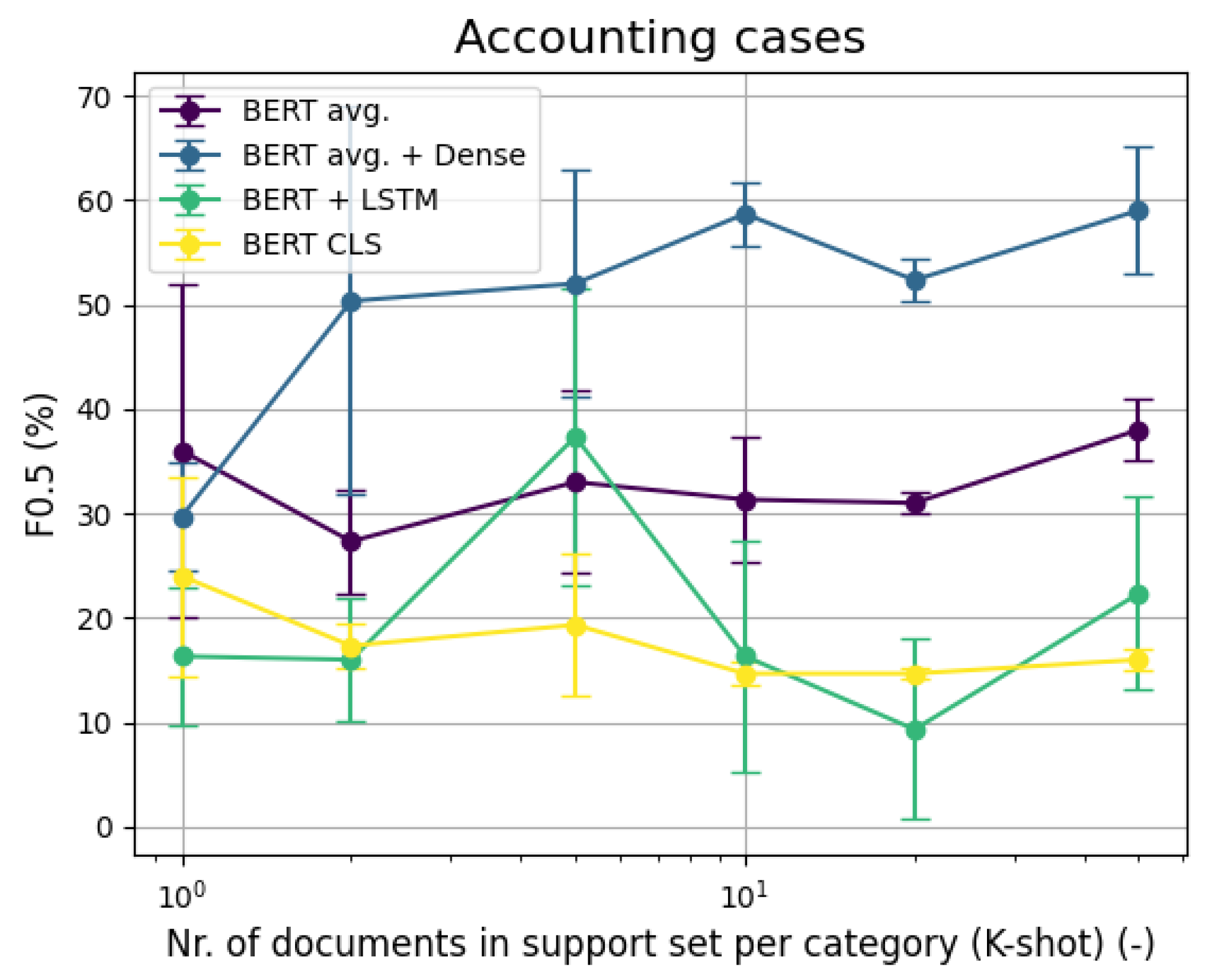
5.1. Few-Shot Binary Classification

The first experiment was performed using the Accounting cases data set introduced in Section 3.2. The aim of this experiment was to measure how effectively the embeddings gained from the Siamese networks could be used when only a few labeled documents are available. The dataset was split in a stratified manner keeping 80% of the data as the training set and 20% as the test set. We randomly sampled positive and negative examples from the training set in a 1:1 ratio and trained a logistic regression classifier on the selected data. The trained classifier was evaluated on the test set. This process was repeated 5 times for each setting. The number of sampled positive and negative documents were 1, 2, 5, 10, 20, 50, 100, and 180 (all data), respectively.

To provide a fair comparison, besides the Siamese networks, we also tested how the BERT CLS vectors and the average of sentence BERT CLS vectors would perform in this task with the same amount of data. The main difference between these models comes from the fact that the huBERT model is only capable of covering 512 tokens at a time, and not dealing with the rest. Although on average 85% of the document tokens are covered by the 512 tokens (see Table 1), also there is a possibility of losing important information. This was addressed by splitting the documents into sentences, vectorizing, and averaging the vectors for a document representation that covered above 99.9% of the dataset on the token level.

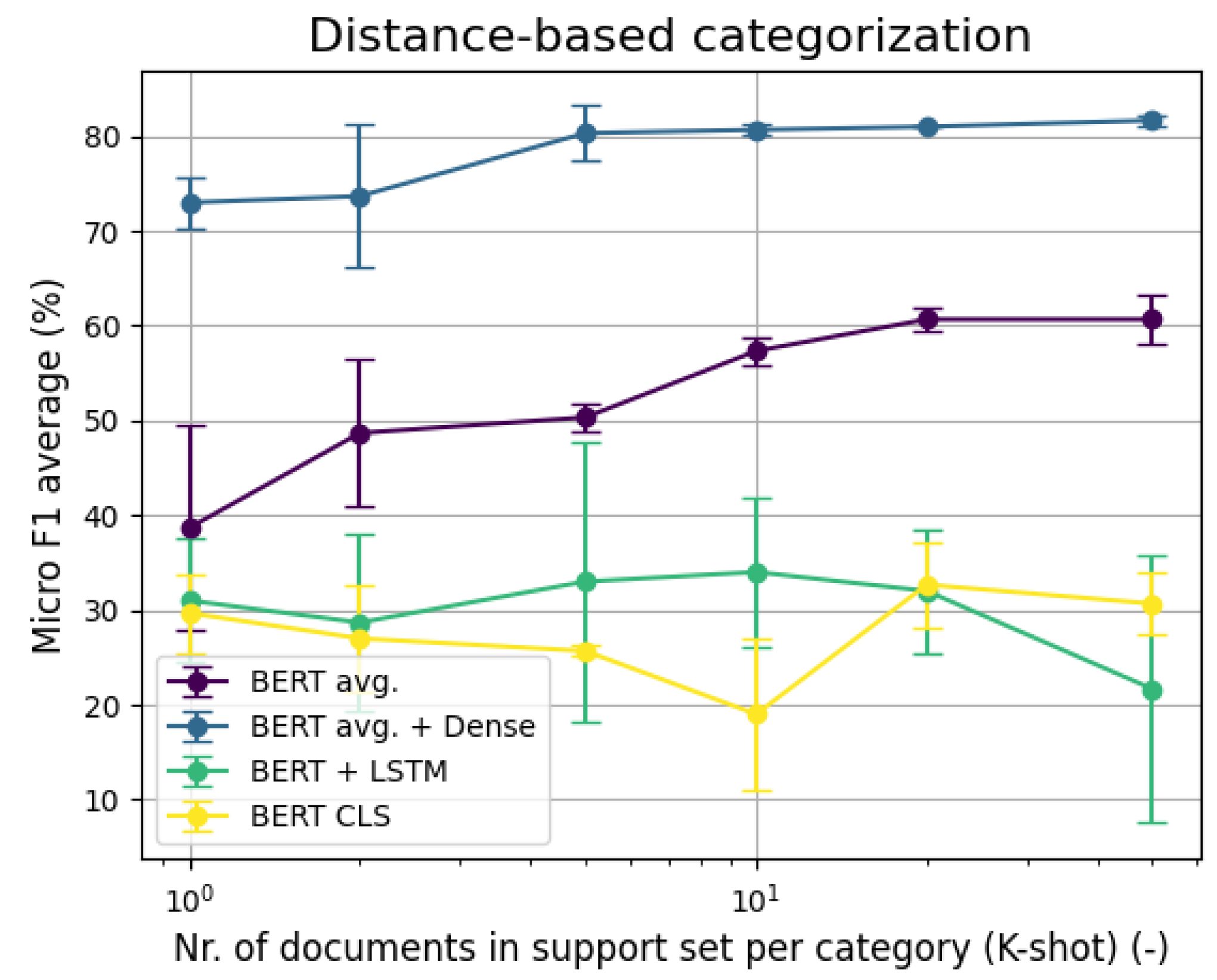
5.2. Few Shot Multi-Label Classification

The aim of the second experiment was to test how the Siamese embeddings would perform in a non-binary, multi-label few-shot classification setting. During the test, the test dataset containing 409 documents was used. This dataset is fully labeled, not just in a binary manner as the Accounting cases dataset.

Since we had 11 different categories (the Accounting cases category included) we performed 11-way K-shot learning setting K to 1, 2, 5, 10, 20, and 50.

The support set selection was performed as follows. Since one document could have more labels, it could also belong to multiple support set categories. However, this could result in more difficultly distinguishable categories in cases when the overlap with another category is high. Hence, only documents with single labels were used as support set elements. The support set was selected from the training set containing 675 documents. When the count of the available documents was sufficient, the sampling was performed without replacing, when not, with replacing. The elements of the support set were vectorized and averaged for each category, respectively. Since the selection of the samples in the support set has an effect on the results we repeated this process three times and averaged the results.

The categorization was performed as follows. The document to be categorized was vectorized and the Euclidean distances to the support set vectors were calculated. In the case of multi-class classification selecting the closest category makes the categorization process straightforward since in this case, the document is classified as the closest label. However, when performing multi-label classification either the number of the classes should be known or the training of an additional sigmoid layer on the distances is required.

An example is shown in Figure 3. The vectors for the support set elements are black, and with red color, the query document is shown. It can be seen that the red triangle is closest to the Tax matters/Personal income tax category, and since the document had only one label originally, it is labeled with this label.

For the sake of simplicity, we assumed that the number of correct labels is known. Hence, during categorization, the closest n number of labels was added to a given document where n is the number of labels of the true label.

6. Results and Discussion

6.1. Few-Shot Binary Classification

The results of the first experiment are shown in Figure 4. As an evaluation metric, $F_{0.5}$ was chosen, which is also calculated from the precision and recall values but puts more weight on precision. This is because, in a production system, the users would prefer accurate labels for the documents, instead of obtaining all labels, as shown in Orosz et al. [39], and Csányi et al. [35]. The reason for not having any variance in the case of the last results is that all of the available data was used for training.

The Siamese networks did not produce the expected results in either case. Head-to-head, the two types of BERT approaches proved to be the best: BERT CLS vector (indicated correspondingly as ’BERT CLS’ in Figure 4), and BERT CLS vectors of sentences averaged (’BERT avg’ in Figure 4). Both cases were generally within standard deviations and produced increasing $F_{0.5}$ values as the training samples increased, reaching 75.8% and 77.3%, respectively. The BERT + LSTM approach reached only 66.04% while the BERT avg. + Dense approach could only reach 59.34% $F_{0.5}$ score using all training data available.

According to the results, the vector representations gained from Siamese networks did not meet the original expectations, because these models could not provide a valuable vector representation for a previously unseen label compared to BERT CLS-based vectors. Nevertheless, in the case of the LSTM approach, this could result from not feeding the LSTM networks by the context-aware word piece embeddings. Another factor explaining this phenomenon could be the transferred knowledge of the BERT model [40] that was not present in the LSTM architecture. Nevertheless, this does not explain the inferiority of the BERT avg. + Dense approach.

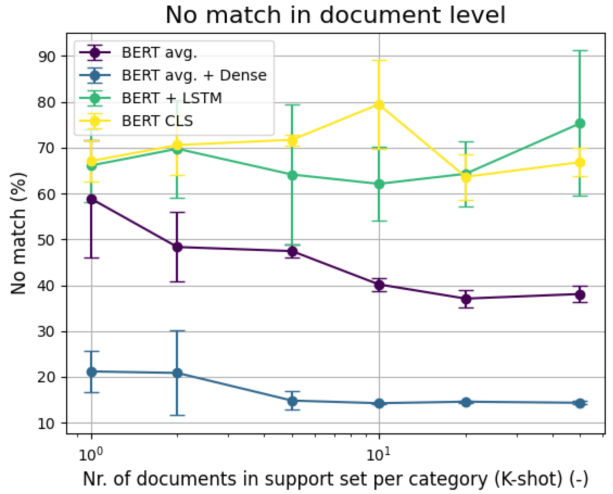
6.2. Few-Shot Multi-Label Classification

The results of the second investigation are shown below. As evaluation metrics, the micro average $F_1$ value, the percentage of non-matching documents, and the $F_{0.5}$ value of the Accounting cases label were selected. The percentage of non-matching documents was calculated by counting the documents that did not share at least one common label in the predicted and actual labels.

Figure 5 shows the effect of increasing the number of elements in the support set on the micro average $F_1$ metric of the different approaches. It can be seen that the Siamese BERT avg. + Dense solution performed by far the best, reaching a micro $F_1$ mean of 80% already at K = 5, which increased only slightly thereafter as K increased. Interestingly, the BERT CLS and the BERT + LSTM solutions did not perform better with increasing K, while BERT avg. moderately increased.

Figure 6 shows the effect of increasing the number of support set elements on the $F_{0.5}$ metric measured on Accounting cases. An increasing trend was only observed for the Siamese BERT avg. + Dense solution, while in the other cases the $F_{0.5}$ of the labeling tended to stagnate or decrease. This leads to the conclusion that the Siamese LSTM + Dense network could not provide a good Siamese model for this task either. It is also worth noting that the BERT avg. + Dense Siamese network was not trained with hardened sampling, which might have improved its performance even more.

Figure 7 shows the effect of increasing the number of support set elements on the percentage of non-matching documents alongside the different approaches. It can be seen that the Siamese network trained on BERT averages performed best, in all cases significantly outperforming the other solutions. After 10 samples, it only failed around 15 out of 100 at the document level, which is also a good result. Note that this evaluation is strict when hierarchical labels are involved since even if misclassification happens between hierarchically connected labels, it is counted as a bad classification although the results are clearly not as bad as confusing with another, hierarchically not connected label.

The experiment of few-shot multi-label classification yielded completely different results compared to the binary classification. At this task by a high margin, the Siamese network fed with averaged BERT sentence vectors proved to be the best approach on all tasks.

6.3. Comparison with Classical Classifiers

In order to put the few-shot multi-label classification results into context we also compared them to the classical tf-idf and logistic regression-based classifiers described in Section 4.1. The results can be seen in

Table 6. Comparison of classical and few-shot approaches.

Approach	Micro ${\mathit{F}}_1$	Macro ${\mathit{F}}_1$	Accounting	Document Level
			Cases $F_{0.5}$	Complete Match	Partly Match	No Match
Classical	88.66%	76.62%	53.19%	77.49%	16.49%	6.02%
Few-shot	81.67%	68.33%	59.00%	78.73%	6.93%	14.35%

. The best results are highlighted with bolding. ’Few-shot’ in the table means the BERT avg.+Dense solution with distance-based classification using 50 examples per category in the support set.

The results show that in some metrics the few-shot approach could surpass the tested classical tf-idf and logistic regression-based method. This clearly shows the power of the few-shot approach since the classical classifiers were trained on nearly 175,000 documents before being further trained on the dataset presented in this paper. Moreover, the few-shot model has not even been trained on the Accounting cases label and even this way it was better by 6.78% in $F_{0.5}$ score on this label. Not to mention that the percentage of perfectly labeled documents was also better by 1.24%. However, in micro average $F_1$ score the classical method performed better by almost 7%, while in macro average $F_1$ by 8.29%.

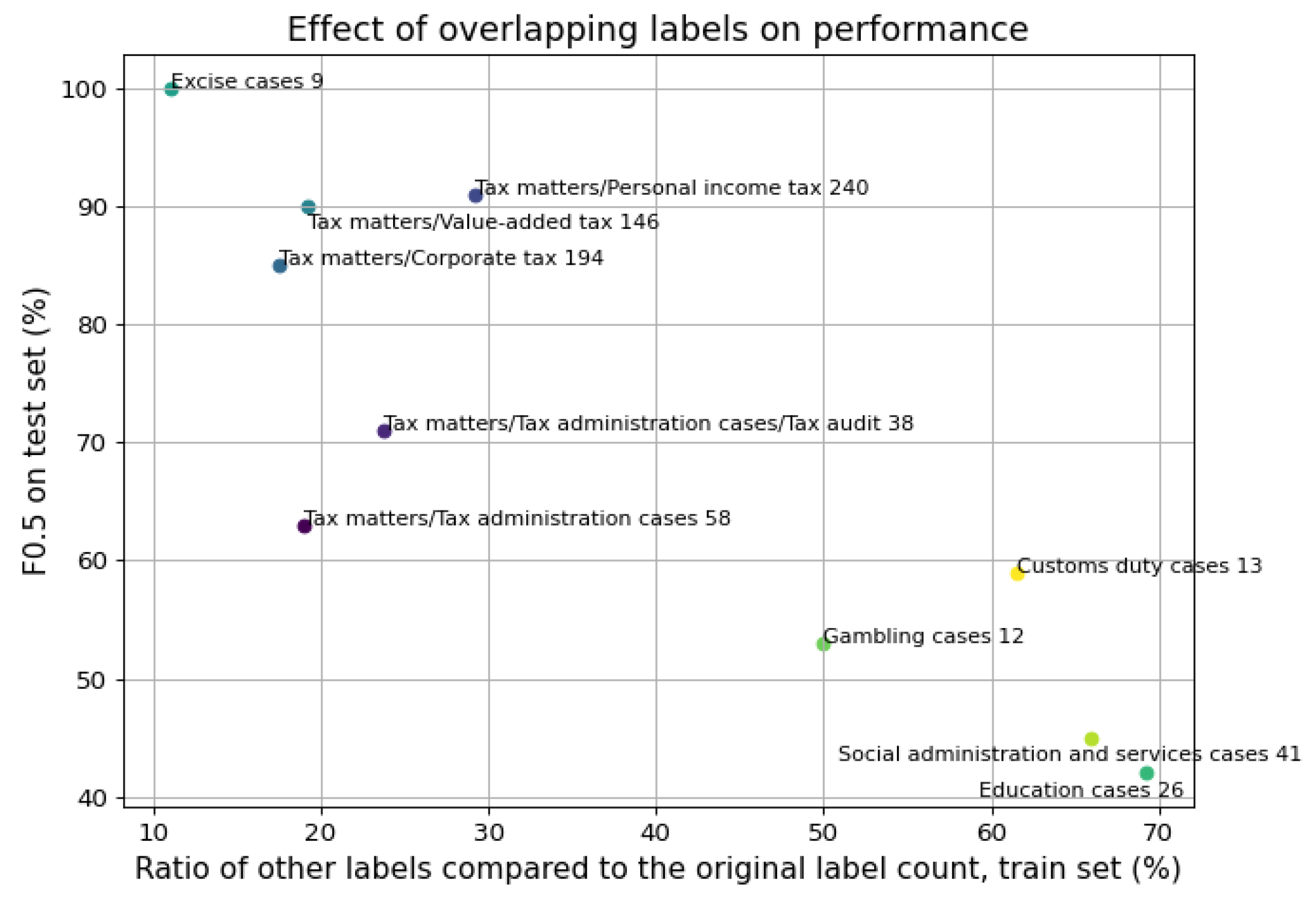
6.4. Effect of Overlapping Labels on Triplet-Trained Siamese Networks for Multi-Label Classification

Although there are few-shot training approaches that support multi-label categorizing scenarios by definition [24] our results suggest that Siamese networks trained with triplet loss can be also applied using distance-based classification using restricted sampling. This approach was designed to tackle multi-class-type problems, not multi-label-type ones. In fact, it is not trivial why the triplet-loss-based approach works. The Siamese net trained with triplets ensures that each document belonging to the same category is mapped close to each other. However, when one document belongs to multiple categories these categories will not be completely separable since there will be a common part, a border in the embedding space where these documents are. Hence, this also means that the categories that have common labels will be mapped close to each other. This is what makes the distance-based evaluation approach work in a multi-label setting.

However, the level of overlap between labels probably highly affects the usability of triplet training. The results shown in

Table 7. Results on test set with counts and overlaps.

	Precision	Recall	${\mathit{F}}_{0.5}$	Train Count	Test Count	Training Set Overlap	Test Set Overlap
Tax matters/Tax administration cases	0.62	0.67	0.63	58	12	0.19	0.25
Tax matters/Tax administration cases/Tax audit	0.83	0.45	0.71	38	11	0.24	0.36
Tax matters/Personal income tax	0.94	0.82	0.91	240	149	0.29	0.15
Tax matters/Corporate Tax	0.83	0.92	0.85	194	103	0.18	0.23
Tax matters/Value-added tax	0.91	0.88	0.90	146	120	0.19	0.18
Excise cases	1.00	1.00	1.00	9	3	0.11	0.00
Education cases	0.38	0.75	0.42	26	4	0.69	1.20
Gambling cases	0.50	0.67	0.53	12	3	0.50	0.33
Social administration and services cases	0.41	0.70	0.45	41	10	0.66	0.50
Accounting cases	0.62	0.66	0.63	N/A	47	N/A	0.74
Customs duty cases	0.57	0.67	0.59	13	6	0.62	1.00

reinforce this statement. This table shows the classification report of the best-performing Siamese approach (50-shot BERT avg.+Dense) on the test set. The table also shows the train and test counts of the labels alongside the overlaps of the labels in the case of the train and test sets. The overlaps were calculated as follows. The columns of the matrix are shown in the heat map in Figure 1. were summed and subtracted 1 from each element of the sum vector. This way, the ratio of other labels that are present alongside a given label can be calculated. Note that this ratio can be higher than one in the case when the given label is present in documents having more than two labels.

Figure 8 shows the $F_{0.5}$ results plotted against the overlap ratios of the training set since this affects the results both during training time and classification time since the support set elements are also selected from this set. The Figure also shows how many documents were present in the training set since this factor affects the results.

The results suggest that by increasing overlap the $F_{0.5}$ score decreases and the majority of the labels are formulating a line. The abundance of labels is another factor that usually affects the results. Although the worst-performing labels usually were the ones with lower abundance, there were two major exceptions: the Excise cases having the lowest abundance performed the best, and the Social administration and services cases performed the second worst while there were five other labels with lower abundance. The worst-performing label, Education cases, was also outperformed by three smaller abundance labels. This suggests that the level of overlap plays a significant role in how the triplet-trained Siamese models perform.

Two labels are somewhat off of the line in Figure 8: Tax administration cases and the Tax administration cases/Tax audit labels. These are the only real hierarchical labels in this dataset. The reason for this is probably that during the evaluation of $F_{0.5}$ these labels can be affected the most because we only calculate perfect matching although it is clear that mixing up a Tax audit label with a Tax administration cases label is not the same as mixing it up with any of the other labels. If we tend to mix these two labels with each other, it can cause both of the results of these labels to decrease.

Another explanation is that hierarchical labels need some extra attention in order to perform optimally. Here, we did not exploit the fact that these labels are hierarchical; thus, when the two closest labels had to be chosen, it could easily happen that both elements of the hierarchy are chosen during classification, which is redundant. Lastly, another explanation could be that the way of training is not working well for hierarchical labels. However, to answer the above-mentioned questions, further investigation is needed.

7. Conclusions

The main research question of this paper was to investigate whether it is possible to train Siamese neural networks using triplet loss with a multi-label setting. The applicability of Siamese networks has been tested in a multi-label categorization setting with hierarchical labels. A test for classifying a previously unseen category was also carried out using a binary dataset. Two Siamese architectures were tested, both BERT-based but one containing only Dense type neural layers and the other containing LSTM layer as well. The research has revealed that triplet-trained Siamese networks can be applied to perform classification but with a restriction of sampling during training. The BERT+Dense Siamese network worked the best to perform the classification on the previously unseen, newly added label in a multi-label categorization setting on every measure ($F_{0.5}$, micro $F_1$ avg., percentage of non-matching documents). However, in a binary classification setting, the Siamese networks underperformed the BERT-based control embeddings by a great margin. The model was able to reach competitive results compared to models trained on tens of thousands of documents using tf-idf vectorization and logistic regression for most of the metrics tested while being trained only on 10 documents. One of the main results is that the level of overlapping with other categories has a negative effect on classification and has a greater effect than the number of labels of each category. Finally, as the research was carried out on a single dataset, further studies are needed to state the conclusions with full certainty; however, the results of the current study provide a good basis for further research.

References

1. Benyus, J.M. Biomimicry: Innovation Inspired by Nature; Morrow: New York, NY, USA, 1997. [Google Scholar]
2. Müller, B.; Reinhardt, J.; Strickland, M.T. Neural Networks: An Introduction; Springer Science & Business Media: Berlin/Heidelberg, Germany, 1995. [Google Scholar]
3. Fei-Fei, L.; Fergus, R.; Perona, P. One-shot learning of object categories. IEEE Trans. Pattern Anal. Mach. Intell. 2006, 28, 594–611. [Google Scholar] [CrossRef]
4. Fink, M. Object classification from a single example utilizing class relevance metrics. Adv. Neural Inf. Process. Syst. 2004, 17, 449–456. [Google Scholar]
5. Wang, Y.; Yao, Q.; Kwok, J.T.; Ni, L.M. Generalizing from a few examples: A survey on few-shot learning. Acm Comput. Surv. 2020, 53, 1–34. [Google Scholar] [CrossRef]
6. Wang, H.; Xu, C.; McAuley, J. Automatic multi-label prompting: Simple and interpretable few-shot classification. arXiv 2022, arXiv:2204.06305. [Google Scholar]
7. Sung, F.; Yang, Y.; Zhang, L.; Xiang, T.; Torr, P.H.; Hospedales, T.M. Learning to compare: Relation network for few-shot learning. In Proceedings of the IEEE Conference on Computer Vision and Pattern Recognition, Salt Lake City, UT, USA, 18–22 June 2018; pp. 1199–1208. [Google Scholar]
8. Garcia, V.; Bruna, J. Few-shot learning with graph neural networks. arXiv 2017, arXiv:1711.04043. [Google Scholar]
9. Snell, J.; Swersky, K.; Zemel, R. Prototypical networks for few-shot learning. Adv. Neural Inf. Process. Syst. 2017, 30, 4077–4087. [Google Scholar]
10. Yan, G.; Li, Y.; Zhang, S.; Chen, Z. Data augmentation for deep learning of judgment documents. In Proceedings of the Intelligence Science and Big Data Engineering, Big Data and Machine Learning: 9th International Conference, IScIDE 2019, Nanjing, China, 17–20 October 2019; Proceedings, Part II 9. Springer: Berlin/Heidelberg, Germany, 2019; pp. 232–242. [Google Scholar]
11. Csányi, G.; Orosz, T. Comparison of data augmentation methods for legal document classification. Acta Tech. Jaurinensis 2022, 15, 15–21. [Google Scholar] [CrossRef]
12. OpenAI. GPT-4 Technical Report. arXiv 2023, arXiv:2303.08774.
13. Chowdhery, A.; Narang, S.; Devlin, J.; Bosma, M.; Mishra, G.; Roberts, A.; Barham, P.; Chung, H.W.; Sutton, C.; Gehrmann, S.; et al. Palm: Scaling language modeling with pathways. arXiv 2022, arXiv:2204.02311. [Google Scholar]
14. Touvron, H.; Lavril, T.; Izacard, G.; Martinet, X.; Lachaux, M.A.; Lacroix, T.; Rozière, B.; Goyal, N.; Hambro, E.; Azhar, F.; et al. Llama: Open and efficient foundation language models. arXiv 2023, arXiv:2302.13971. [Google Scholar]
15. Brown, T.; Mann, B.; Ryder, N.; Subbiah, M.; Kaplan, J.D.; Dhariwal, P.; Neelakantan, A.; Shyam, P.; Sastry, G.; Askell, A.; et al. Language models are few-shot learners. Adv. Neural Inf. Process. Syst. 2020, 33, 1877–1901. [Google Scholar]
16. Wei, J.; Bosma, M.; Zhao, V.Y.; Guu, K.; Yu, A.W.; Lester, B.; Du, N.; Dai, A.M.; Le, Q.V. Finetuned language models are zero-shot learners. arXiv 2021, arXiv:2109.01652. [Google Scholar]
17. Ahmadian, A.; Dash, S.; Chen, H.; Venkitesh, B.; Gou, S.; Blunsom, P.; Üstün, A.; Hooker, S. Intriguing Properties of Quantization at Scale. arXiv 2023, arXiv:2305.19268. [Google Scholar]
18. Chopra, S.; Hadsell, R.; LeCun, Y. Learning a similarity metric discriminatively, with application to face verification. In Proceedings of the 2005 IEEE Computer Society Conference on Computer Vision and Pattern Recognition (CVPR’05), San Diego, CA, USA, 20–26 June 2005; Volumne 1, pp. 539–546. [Google Scholar]
19. Chicco, D. Siamese neural networks: An overview. In Artificial Neural Networks; Springer Nature: Berlin/Heidelberg, Germany, 2021; pp. 73–94. [Google Scholar]
20. Weinberger, K.Q.; Saul, L.K. Distance metric learning for large margin nearest neighbor classification. J. Mach. Learn. Res. 2009, 10, 207–244. [Google Scholar]
21. Schroff, F.; Kalenichenko, D.; Philbin, J. Facenet: A unified embedding for face recognition and clustering. In Proceedings of the IEEE Conference on Computer Vision and Pattern Recognition, Boston, MA, USA, 7–12 June 2015; pp. 815–823. [Google Scholar]
22. Cheng, K.H.; Chou, S.Y.; Yang, Y.H. Multi-label few-shot learning for sound event recognition. In Proceedings of the 2019 IEEE 21st International Workshop on Multimedia Signal Processing (MMSP), Kuala Lumpur, Malaysia, 27–29 September 2019; pp. 1–5. [Google Scholar]
23. Devlin, J.; Chang, M.W.; Lee, K.; Toutanova, K. Bert: Pre-training of deep bidirectional transformers for language understanding. arXiv 2018, arXiv:1810.04805. [Google Scholar]
24. Simon, C.; Koniusz, P.; Harandi, M. Meta-learning for multi-label few-shot classification. In Proceedings of the IEEE/CVF Winter Conference on Applications of Computer Vision, Waikoloa, HI, USA, 3–8 January 2022; pp. 3951–3960. [Google Scholar]
25. Rios, A.; Kavuluru, R. Few-shot and zero-shot multi-label learning for structured label spaces. In Proceedings of the Conference on Empirical Methods in Natural Language Processing, Conference on Empirical Methods in Natural Language Processing; NIH Public Access: Brussels, Belgium, 2018; Volume 2018, p. 3132. [Google Scholar]
26. Vaswani, A.; Shazeer, N.; Parmar, N.; Uszkoreit, J.; Jones, L.; Gomez, A.N.; Kaiser, Ł.; Polosukhin, I. Attention is all you need. Adv. Neural Inf. Process. Syst. 2017, 30, 5998–6008. [Google Scholar]
27. Kipf, T.N.; Welling, M. Semi-supervised classification with graph convolutional networks. arXiv 2016, arXiv:1609.02907. [Google Scholar]
28. Chalkidis, I.; Fergadiotis, M.; Malakasiotis, P.; Aletras, N.; Androutsopoulos, I. Extreme multi-label legal text classification: A case study in EU legislation. arXiv 2019, arXiv:1905.10892. [Google Scholar]
29. Chalkidis, I.; Fergadiotis, M.; Malakasiotis, P.; Androutsopoulos, I. Large-scale multi-label text classification on EU legislation. arXiv 2019, arXiv:1906.02192. [Google Scholar]
30. Chung, J.; Gulcehre, C.; Cho, K.; Bengio, Y. Empirical evaluation of gated recurrent neural networks on sequence modeling. arXiv 2014, arXiv:1412.3555. [Google Scholar]
31. Sumbul, G.; Ravanbakhsh, M.; Demir, B. Informative and representative triplet selection for multilabel remote sensing image retrieval. IEEE Trans. Geosci. Remote. Sens. 2021, 60, 1–11. [Google Scholar] [CrossRef]
32. Biswas, S.; Gall, J. Multiple Instance Triplet Loss for Weakly Supervised Multi-Label Action Localisation of Interacting Persons. In Proceedings of the IEEE/CVF International Conference on Computer Vision, Montreal, QC, Canada, 11–17 October 2021; pp. 2159–2167. [Google Scholar]
33. Melsbach, J.; Stahlmann, S.; Hirschmeier, S.; Schoder, D. Triplet transformer network for multi-label document classification. In Proceedings of the 22nd ACM Symposium on Document Engineering, San Jose, CA, USA, 20–23 September 2022; pp. 1–4. [Google Scholar]
34. Nemeskey, D.M. Introducing huBERT. In Proceedings of the XVII. Magyar Számítógépes Nyelvészeti Konferencia (MSZNY2021), Szeged, Hungary, 28–29 January 2021; pp. 3–14. [Google Scholar]
35. Csányi, G.M.; Vági, R.; Nagy, D.; Üveges, I.; Vadász, J.P.; Megyeri, A.; Orosz, T. Building a Production-Ready Multi-Label Classifier for Legal Documents with Digital-Twin-Distiller. Appl. Sci. 2022, 12, 1470. [Google Scholar] [CrossRef]
36. Ghamrawi, N.; McCallum, A. Collective multi-label classification. In Proceedings of the 14th ACM International Conference on Information and Knowledge Management, Bremen, Germany, 31 October–5 November 2005; pp. 195–200. [Google Scholar]
37. Pedregosa, F.; Varoquaux, G.; Gramfort, A.; Michel, V.; Thirion, B.; Grisel, O.; Blondel, M.; Prettenhofer, P.; Weiss, R.; Dubourg, V.; et al. Scikit-learn: Machine learning in Python. J. Mach. Learn. Res. 2011, 12, 2825–2830. [Google Scholar]
38. Hochreiter, S.; Schmidhuber, J. Long short-term memory. Neural Comput. 1997, 9, 1735–1780. [Google Scholar] [CrossRef]
39. Orosz, T.; Vági, R.; Csányi, G.M.; Nagy, D.; Üveges, I.; Vadász, J.P.; Megyeri, A. Evaluating Human versus Machine Learning Performance in a LegalTech Problem. Appl. Sci. 2021, 12, 297. [Google Scholar] [CrossRef]
40. Ranaldi, L.; Ruzzetti, E.S.; Zanzotto, F.M. PreCog: Exploring the Relation between Memorization and Performance in Pre-trained Language Models. arXiv 2023, arXiv:2305.04673. [Google Scholar]
Figure 1. Heat map of the overlapping labels in the training set.
Information 14 00520 g001
Figure 2. Siamese architectures, (a) Average of BERT CLS vectors of sentences with a dense layer; (b) BERT word piece embeddings with bidirectional LSTM and dense layers.
Information 14 00520 g002
Figure 3. Categorization based on distance.
Information 14 00520 g003
Figure 4. Comparison of few-shot learning methods on Accounting cases (binary data).
Information 14 00520 g004
Figure 5. Micro average F 1 of classification by increasing support set (multi-labeled data).
Information 14 00520 g005
Figure 6. F 0.5 of Accounting cases classification by increasing support set (multi-labeled data).
Information 14 00520 g006
Figure 7. Percentage of falsely labeled documents by increasing support set.
Information 14 00520 g007
Figure 8. Effect of overlapping labels on test set F 0.5 performance, training set overlaps.
Information 14 00520 g008