A Method for UWB Localization Based on CNN-SVM and Hybrid Locating Algorithm

Abstract

In this paper, aiming at the severe problems of UWB positioning in NLOS-interference circumstances, a complete method is proposed for NLOS/LOS classification, NLOS identification and mitigation, and a final accurate UWB coordinate solution through the integration of two machine learning algorithms and a hybrid localization algorithm, which is called the C-T-CNN-SVM algorithm. This algorithm consists of three basic processes: an LOS/NLOS signal classification method based on SVM, an NLOS signal recognition and error elimination method based on CNN, and an accurate coordinate solution based on the hybrid weighting of the Chan–Taylor method. Finally, the validity and accuracy of the C-T-CNN-SVM algorithm are proved through a comparison with traditional and state-of-the-art methods. (i) Focusing on four main prediction errors (range measurements, maxNoise, stdNoise and rangeError), the standard deviation decreases from 13.65 cm to 4.35 cm, while the mean error decreases from 3.65 cm to 0.27 cm, and the errors are practically distributed normally, demonstrating that after training a SVM for LOS/NLOS signal classification and a CNN for NLOS recognition and mitigation, the accuracy of UWB range measurements may be greatly increased. (ii) After target positioning, the proposed method can realize a one-dimensional X-axis and Y-axis accuracy within 175 mm, and a Z-axis accuracy within 200 mm; a 2D ($X,Y$) accuracy within 200 mm; and a 3D accuracy within 200 mm, most of which fall within (100 mm, 100 mm, 100 mm). (iii) Compared with the traditional algorithms, the proposed C-T-CNN-SVM algorithm performs better in location accuracy, cumulative error probability (CDF), and root-mean-square difference (RMSE): the 1D, 2D, and 3D accuracy of the proposed method is 2.5 times that of the traditional methods. When the location error is less than 10 cm, the CDF of the proposed algorithm only reaches a value of 0.17; when the positioning error reaches 30 cm, only the CDF of the proposed algorithm remains in an acceptable range. The RMSE of the proposed algorithm remains ideal when the distance error is greater than 30 cm. The results of this paper and the idea of a combination of machine learning methods with the classical locating algorithms for improved UWB positioning under NLOS interference could meet the growing need for wireless indoor locating and communication, which indicates the possibility for the practical deployment of such a method in the future.

1. Introduction

The popularity of mobile terminals has grown rapidly as a result of the quick advancement of mobile Internet technology, which has also increased the demand for indoor locations. Collecting data such as location information is a crucial component of ideas such as the Internet of Things or Industry $4.0$. The development of precise positioning and integrated navigation systems has been given more and more attention and has become a hot research topic.

The most widely used indoor locating technologies include wireless LAN, radio frequency tags, ZigBee, Bluetooth, and infrared. These technologies are, however, easily impacted by different indoor noise signals and environments, and complicated inside environments severely influence positioning accuracy.

Comparatively, positioning technology based on ultra-wideband (UWB) has the advantages of high time resolution and high positioning accuracy, which can reach centimeter-level or even millimeter-level positioning [1]. UWB has made considerable progress in recent years and is utilized extensively in both military and civilian industries, such as power generation, healthcare, the chemical industry, tunnel building, hazardous area management, etc. [2,3,4].

Much research has been carried out on UWB indoor location technology [5,6,7,8]. The effectiveness of various locating and tracking algorithms is assessed in [5] using a specific UWB indoor ranging model, and their benefits and downsides concerning various situations and system design characteristics are also investigated. Ref. [6] suggests a technique for using a UWB and fusion algorithm to determine a pedestrian’s indoor location. A description of indoor positioning systems based on UWB technology is given in [7]. Ref. [8] describes a technique for fusing and filtering UWB and IMU (inertial measurement unit) data while tracking the errors of variables such as position, speed, and direction.

When a radio transmitter and radio receiver are in a direct line-of-sight obstruction, this is referred to as non-line-of-sight (NLOS). In this scenario, the sent signal may encounter a penetrating, reflected, or diffracted path on its way to the receiver, lengthening its journey and weakening its signal. As a result, whether the assessment of time or signal intensity is biased determines how far away something is. As NLOS propagation occurs constantly in cities and other built-up areas and is responsible for the signals reaching the various receivers, it is important to consider how NLOS propagation may affect location estimates.

Although UWB technology has good resistance to multipath interference and can achieve centimeter-level positioning accuracy (generally referred to as 2D planar positioning), due to complex and dynamic indoor environments, there are frequently unexpected obstacles that cause NLOS propagation, which introduce error in ranging measurements [9]. Additionally, the UWB transmission signal is highly susceptible to obstruction. When there is a lot of interference, data fluctuate abnormally (typically with a time delay), making indoor placement difficult or even dangerous. Furthermore, when collecting the data, the UWB is unaware of whether the signal is being interfered with. Therefore, it has become vital to find a solution for the challenge of conducting UWB precise positioning while experiencing interference from NLOS signals.

NLOS recognition and NLOS mitigation are two different approaches that have been developed to deal with NLOS errors [10,11,12,13]. In NLOS recognition, an AdaBoost machine learning meta-algorithm-based strong non-line-of-sight propagation classifier is suggested in [14]. A statistical line-of-sight recognition method is put out in [15] that makes use of channel state data to increase the distinction between LOS and NLOS scenarios. In [16], a real-time LOS identification method called “AmpN” based on WiFi is proposed that could work in both stationary and mobile settings. In [17], a LOS/NLOS path recognition method is presented to distinguish between signals sent along the LOS and NLOS path with high accuracy and real-time ability. Convolutional neural networks (CNNs) are used in [18] and are claimed to perform well at detecting four different types of channel impulse response figures and identifying LOS/NLOS channels. As for NLOS mitigation, in [19], several manually extracted channel impulse response properties are checked against the LOS/NLOS likelihood ratio. Ref. [20] proposes a supervised machine learning algorithm-based LOS/NLOS categorization approach. A less environment-dependent and a priori knowledge-independent NLOS identification and mitigation strategy for ranging that can identify the precise NLOS channel is proposed in [19]. A unique approach to NLOS mitigation is put out in [21], which is based on the simple sparse pseudo-input Gaussian process (SPGP) and is claimed to reduce the bias of both LOS and NLOS circumstances without the traditional primary process of NLOS identification. Additionally, the simultaneous localization and tracking (SLAT) problem in non-line-of-sight (NLOS) situations is studied in [22].

However, the majority of existing algorithms that cope with NLOS errors merely focus on either NLOS recognition or NLOS mitigation instead of a complete process from NLOS/LOS classification to identification and then to mitigation. Furthermore, these methods mainly target two-dimensional precision positioning data sets. Currently, in the scenario of wireless indoor locating and communication, there is a lack of an effective algorithm that could simultaneously improve the one-dimensional, two-dimensional as well as three-dimensional location accuracy under NLOS/LOS hybrid circumstances.

Meanwhile, numerous studies have been carried out on indoor localization based on either classical algorithms such as Chan and Taylor or machine learning methods such as SVM and CNN [23,24,25,26,27,28,29]. However, there exist certain limitations when applying any of the above algorithms alone, especially in the studied scenario of this paper, wireless indoor locating and communications under severe NLOS interference. As for various machine learning algorithms, which have been widely used for indoor precision positioning in recent years, these methods merely improve the accuracy or usefulness of existing positioning methods, which can hardly cover the entire goal of this paper. In addition, the positioning accuracy of the traditional Chan algorithm will be significantly impacted if the Fresnel zone is blocked by more than 50 percent. While the traditional Taylor algorithm requires the initial estimated position of unknown nodes, if the initial value is inappropriate, such a method is likely to fail to converge. Furthermore, the existing research on Chan and Taylor for indoor localization mainly focuses on 2D precision under weak NLOS interference or in a non-NLOS environment.

Considering this, to effectively mitigate signal propagation errors in indoor positioning and communication under strong NLOS interference, this paper presents a complete method for NLOS/LOS classification and NLOS identification and mitigation through the integration of two machine learning algorithms and a hybrid localization algorithm. In this paper, we choose the method of SVM for LOS/NLOS signal classification, the method of CNN for NLOS signal recognition and error elimination, and the hybrid weighting of the Chan–Taylor method for the final accurate UWB coordinate solution, which fully utilizes the advantages of the above mature methods.

First and foremost, by adopting the principle of structural risk minimization to solve non-linear regression problems, SVMs could transform non-linear classification into linear classification in high-dimensional space under high-dimensional space substitution, which performs well in solving problems such as classification and pattern recognition. In view of this, in our C-T-CNN-SVM algorithm, we choose SVM for LOS/NLOS signal classification, as the SVM-based technique can identify and distinguish NLOS signals in UWB-ranging information with high accuracy through preliminary learning and training, thus achieving an accurate classification of LOS and NLOS signals during the primary step.

On this basis, as a CNN can classify input material that is translation-invariant according to its hierarchical structure and has the capacity for representation learning, we train a specific CNN structure for NLOS recognition and mitigation, which will greatly increase the accuracy of UWB range measurements.

After that, as for the final accurate UWB coordinate solution, the most widely used algorithm, Chan and Taylor, is selected. The reasons for this are as follows. The traditional Chan algorithm is a non-recursive method for solving a hyperbolic system of equations with high positioning precision, little computation, and a clear expression result in accordance with the function. Additionally, a recursive process method such as the Taylor algorithm could enhance the predicted position of unknown nodes by resolving the local least-squares solution of the measurement error in each iteration. The Chan method is therefore used in this study as the initial algorithm for positioning to produce a relatively accurate initial solution coordinate of anchor points and to simplify the convergence of the Taylor algorithm, thereby reducing the complexity of the operation and increasing operational efficiency. By combining the Chan and Taylor approaches with carefully selected weighting indexes, we can fully utilize their advantages while avoiding their drawbacks, such as the deteriorated positioning accuracy of the Chan algorithm when the Fresnel zone is severely blocked and the non-convergence of the Taylor algorithm if the initial value is inappropriate.

Simulation and experimental results in the later part of this paper have demonstrated the effectiveness of our C-T-CNN-SVM algorithm and how each part of our algorithm works to execute a rather accurate UWB indoor positioning under severe NLOS interference. To the best of our knowledge, this is the first time a hybrid of classical localization algorithms is combined with emerging machine learning algorithms, which realizes LOS/NLOS signal classification and NLOS recognition and elimination under strong NLOS interference.

The main contributions of this paper are summarized as follows.

(i)

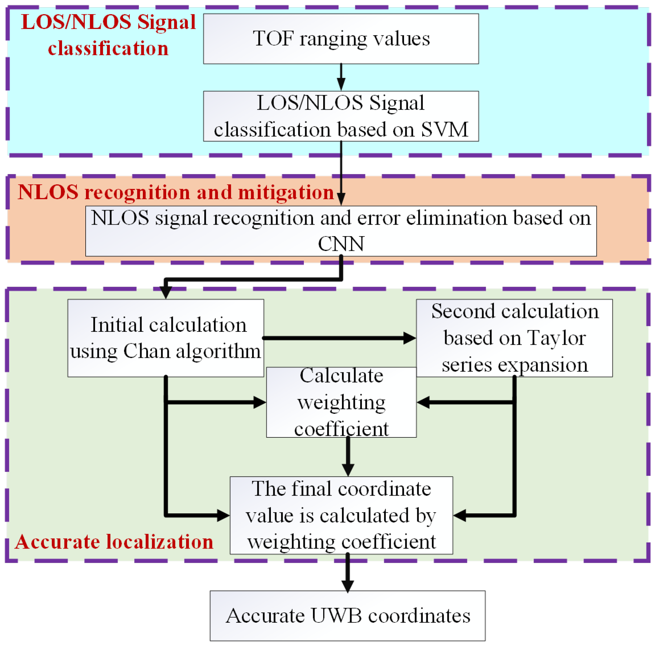
A complete method is proposed for NLOS/LOS classification and NLOS identification and mitigation, and a final accurate UWB coordinate solution is proposed through the integration of two machine learning algorithms and a hybrid localization algorithm, which can effectively mitigate signal propagation errors in indoor positioning and communication under strong NLOS interference. We call this innovative algorithm the C-T-CNN-SVM algorithm, which consists of three basic processes: an LOS/NLOS signal classification method based on SVM, an NLOS signal recognition and error elimination method based on CNN, and an accurate coordinate solution based on the hybrid weighting of the Chan–Taylor method.

(ii)

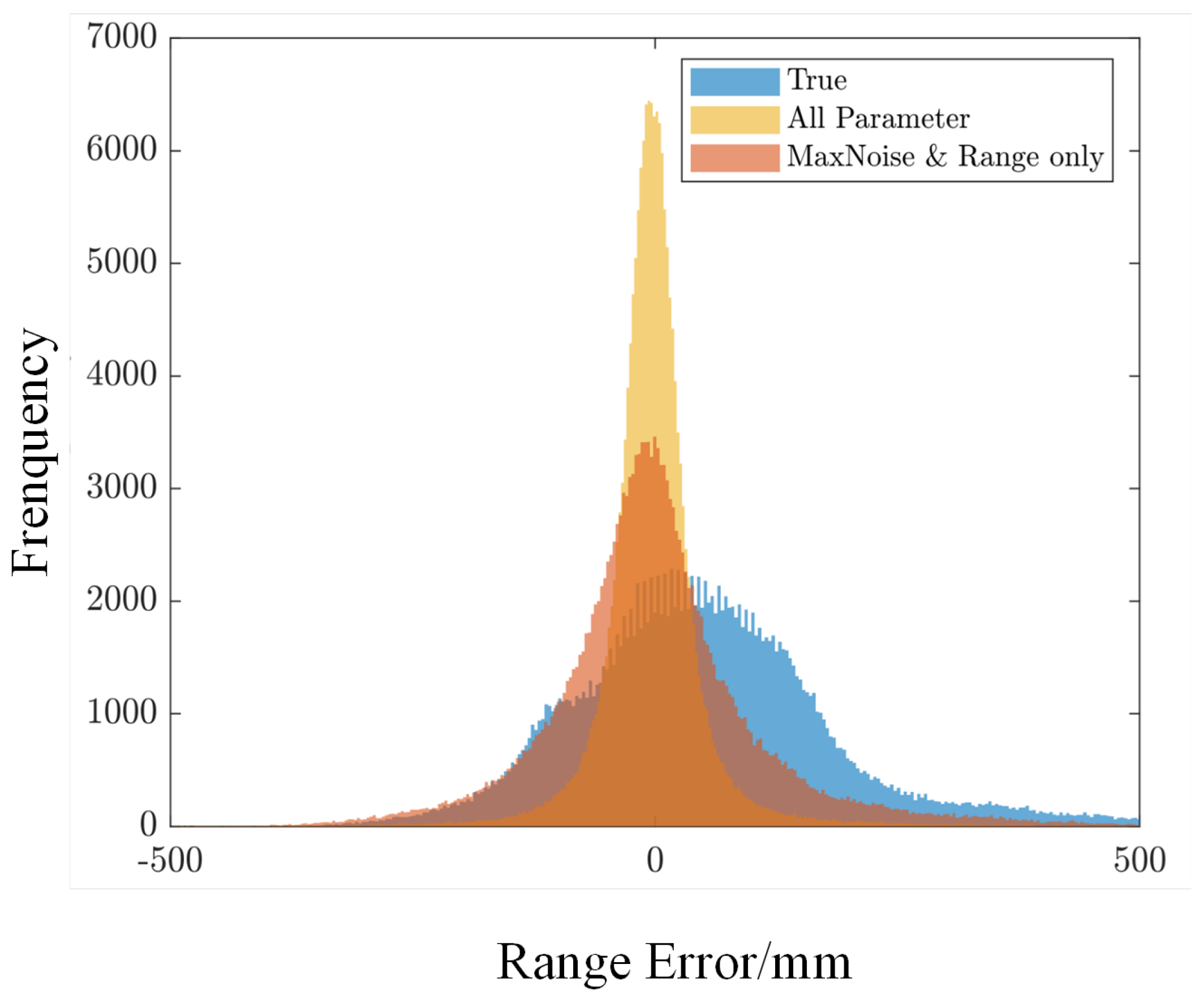
After LOS/NLOS signal classification based on SVM and the CNN-based method for NLOS signal recognition and error elimination, using the testing data set and focusing on four main prediction errors (range measurements, maxNoise, stdNoise and rangeError), the standard deviation decreases from 13.65 cm to 4.35 cm, while the mean error decreases from 3.65 cm to 0.27 cm, and the errors are practically distributed normally, which demonstrates that after training a CNN for NLOS recognition and performing NLOS mitigation, the accuracy of UWB range measurements may be greatly increased.

(iii)

During the final accurate UWB coordinate solution based on the hybrid weighting of the Chan and Taylor algorithms, using a total number of 648 testing data sets that vary in the percentage of LOS and NLOS signals, after target positioning, this method can realize a one-dimensional X-axis and Y-axis accuracy within 175 mm and a Z-axis accuracy within 200 mm; a 2D ($X,Y$) accuracy within 200 mm; and a 3D accuracy within 200 mm, most of which fall within (100 mm, 100 mm, 100 mm).

(iv)

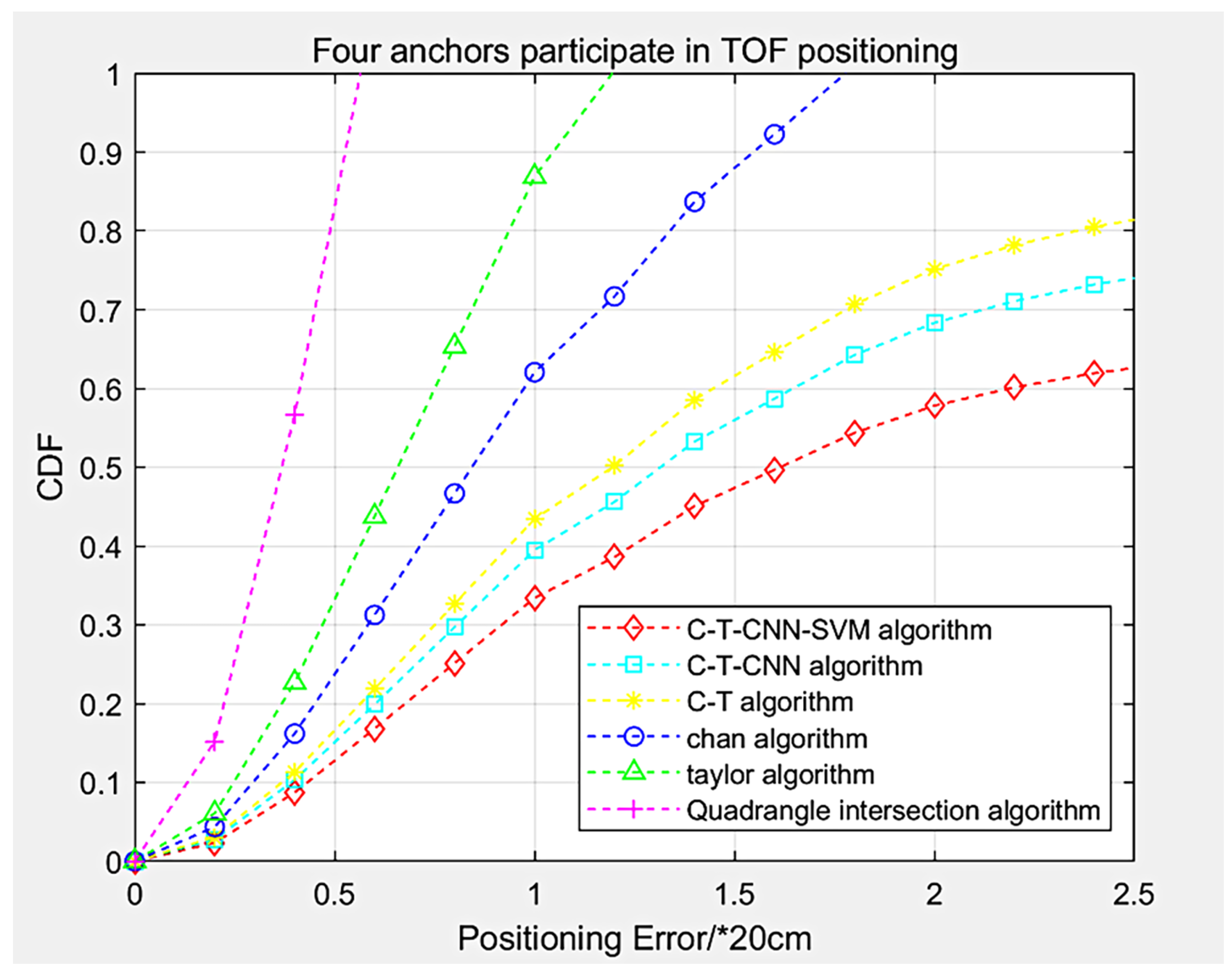
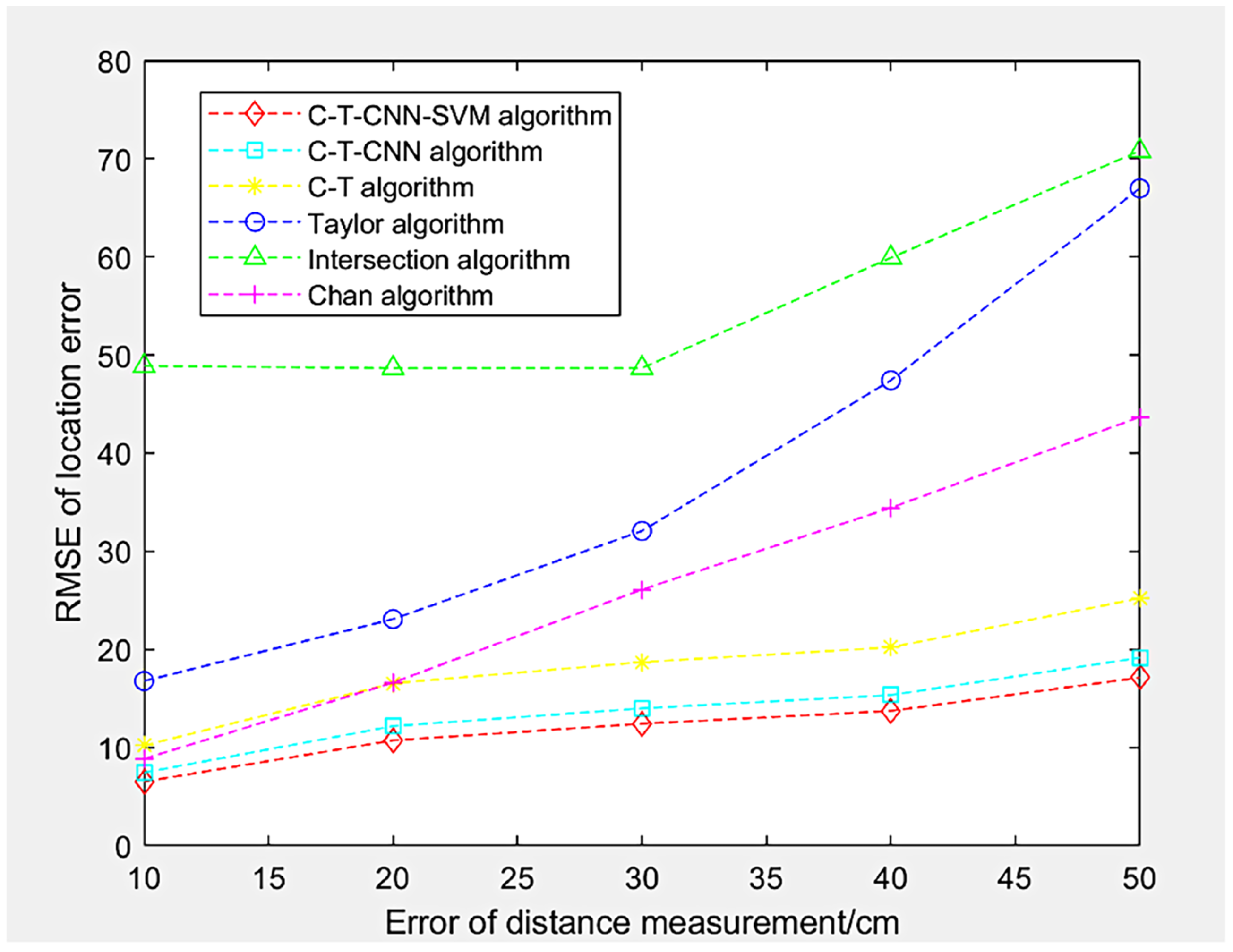
Compared with the traditional Chan algorithm, Taylor algorithm, and intersection algorithm error, the proposed C-T-CNN-SVM algorithm performs better in location accuracy, cumulative error probability (CDF), and root-mean-square difference (RMSE): the 1D, 2D, and 3D accuracy of the proposed method is 2.5 times that of the traditional methods; when the location error is less than 10 cm, the CDF of the proposed algorithm only reaches $0.17$, while that of the four-side intersection algorithm is as high as $0.85$. When the positioning error reaches 30 cm, only the CDF of the proposed algorithm remains in an acceptable range; the RMSE of the proposed algorithm remains ideal when the distance error is greater than 30 cm, while that of the traditional algorithms grow very large when the distance error exceeds 10 cm.

(v)

The research result of this paper and the idea of a combination of machine learning methods with the classical locating algorithms for an improved UWB positioning under NLOS interference could meet the growing need for wireless indoor locating and communication, which indicates the possibility for the practical deployment of such a method in the future.

The rest of this paper is organized as follows.

(i)

As stated in Section 2, we first create the UWB positioning model. From there, we investigate the NLOS error in the model and introduce standard UWB algorithms as well as the SVM and CNN technology that will be used in our method.

(ii)

The C-T-CNN-SVM algorithm, a particular UWB positioning technique, is described in detail in Section 3. It is separated into three sections: LOS/NLOS signal classification based on SVM, NLOS signal recognition and classification based on CNN, and final accurate UWB localization based on a hybrid locating algorithm.

(iii)

In Section 4, performance analysis and experimental findings are presented.

(iv)

Final remarks can be found in Section 5.

2. System Model, Assumptions and Notations

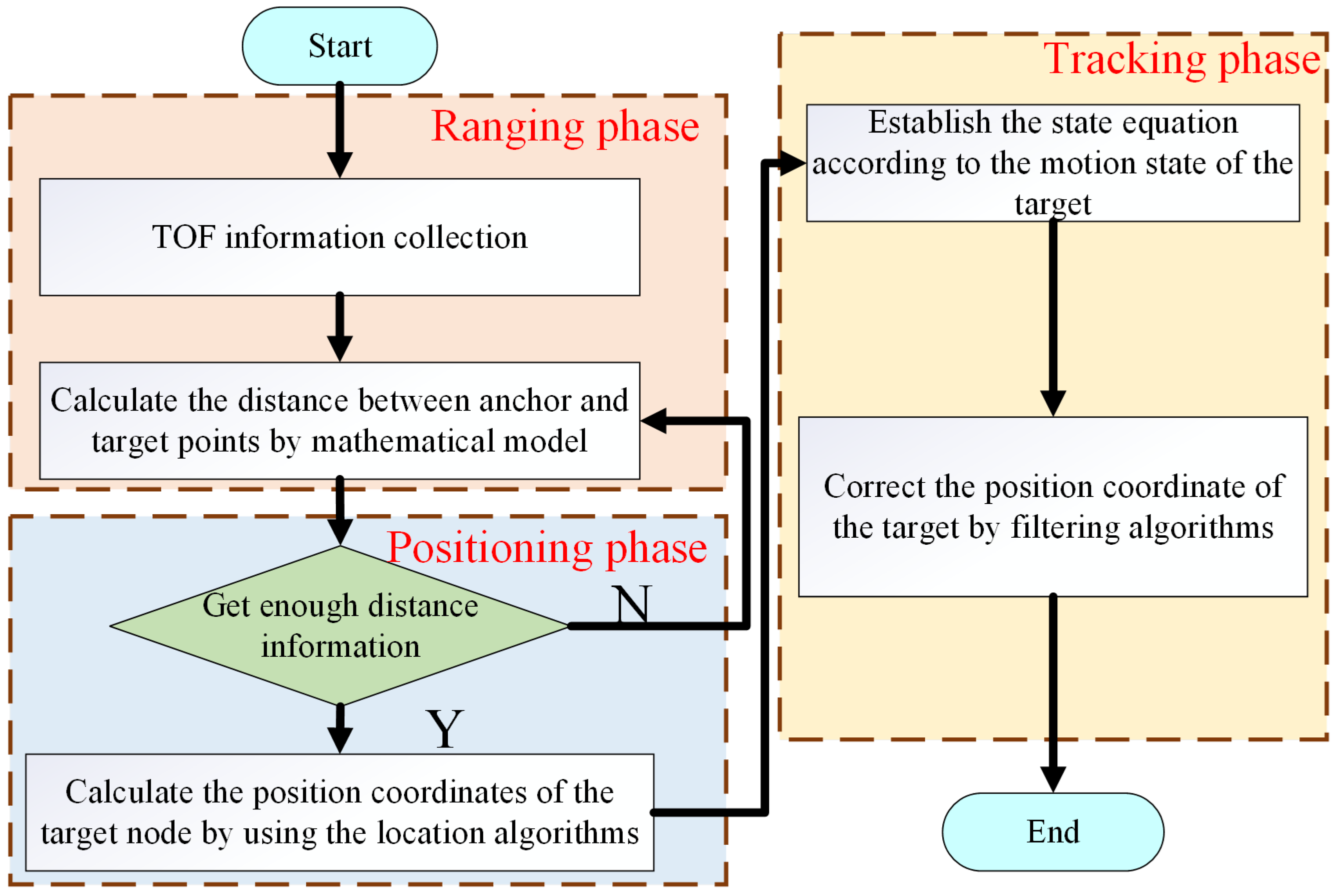
2.1. The Overall Model of Accurate UWB Localization

As shown in Figure 1, for the indoor UWB positioning technology based on TOF ranging, its positioning process can be mainly divided into three stages: the ranging stage, the positioning stage, and the tracking stage. In the ranging stage, the anchor and the target node establish communication to obtain some necessary ranging information, such as time, signal strength, etc. Then, the distance between the anchor point and the target node is calculated by the TOF model. In the positioning stage, when the distance value meets certain conditions, the geometric positioning algorithm is used to calculate the position coordinates of the target node. In the tracking stage, the position coordinates of the target nodes are corrected by the filtering algorithm after setting up appropriate state equations of the target motion and initializing the filtering parameters.

In this paper, the main research point is the second stage, the positioning stage. It focuses on the analysis of the shortcomings of the existing positioning technology at this stage. On this basis, machine learning technologies such as SVM and CNN are introduced to achieve better classification, recognition, and elimination capabilities of NLOS signals. At the same time, the positioning accuracy of the processed positioning signal is further improved based on the hybrid weighted positioning algorithm. The detailed implementation principles of the above ideas will be analyzed and demonstrated in the following chapters.

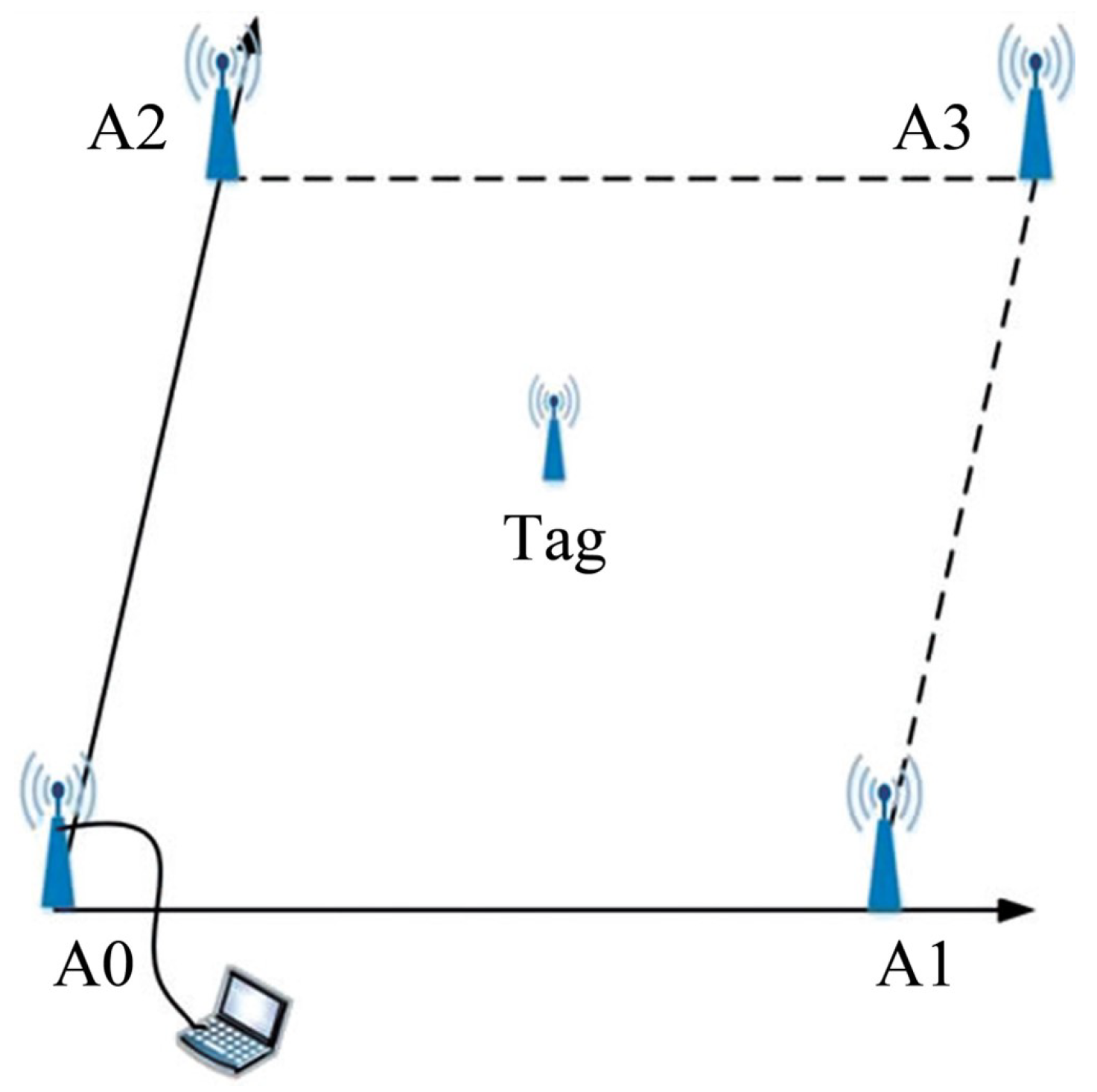
2.2. UWB Model Studied in This Paper

There are four anchor points, $A_i(i=0,1,2,3)$, and one target Tag in the three-dimensional area under study in this research. Figure 2 displays the positioning diagram based on UWB.

The time-of-flight ranging method (TOF) is used in this paper’s UWB positioning model to obtain the values $d_1,d_2,d_3,d_4$. Figure 3 illustrates the TOF range theory. The transmitter is the component that sends the TOF ranging signal, while the receiving end is the component that receives the ranging signal and requires the UWB location. The arrows in the diagram merely show the general direction of sending and returning TOF signals, not their exact directions.

Using the time of flight of the data signal between a pair of transceivers and back, this method, known as two-way ranging, calculates the distance between two sites. While the time interval between data signals received by the receiver and response signals issued by the transmitter is denoted as $T_r$, it is $T_t$ between data signals sent by the transmitter and response signals received by the transmitter. The signal’s one-way travel time between the transceiver pair is:

$$T_f=\left(T_t-T_r\right)/2$$

(1)

The distance between two points is:

$$d=c\times T_f$$

(2)

where c denotes the electromagnetic wave’s propagation speed. However, the fundamental drawback of the TOF range is that it is susceptible to environmental influences. The ranging error increases in direct proportion to time deviation. Because of this, the TOF range frequently contains a significant amount of inaccuracy in complex environments, which is the key issue this research attempts to resolve through precise UWB positioning.

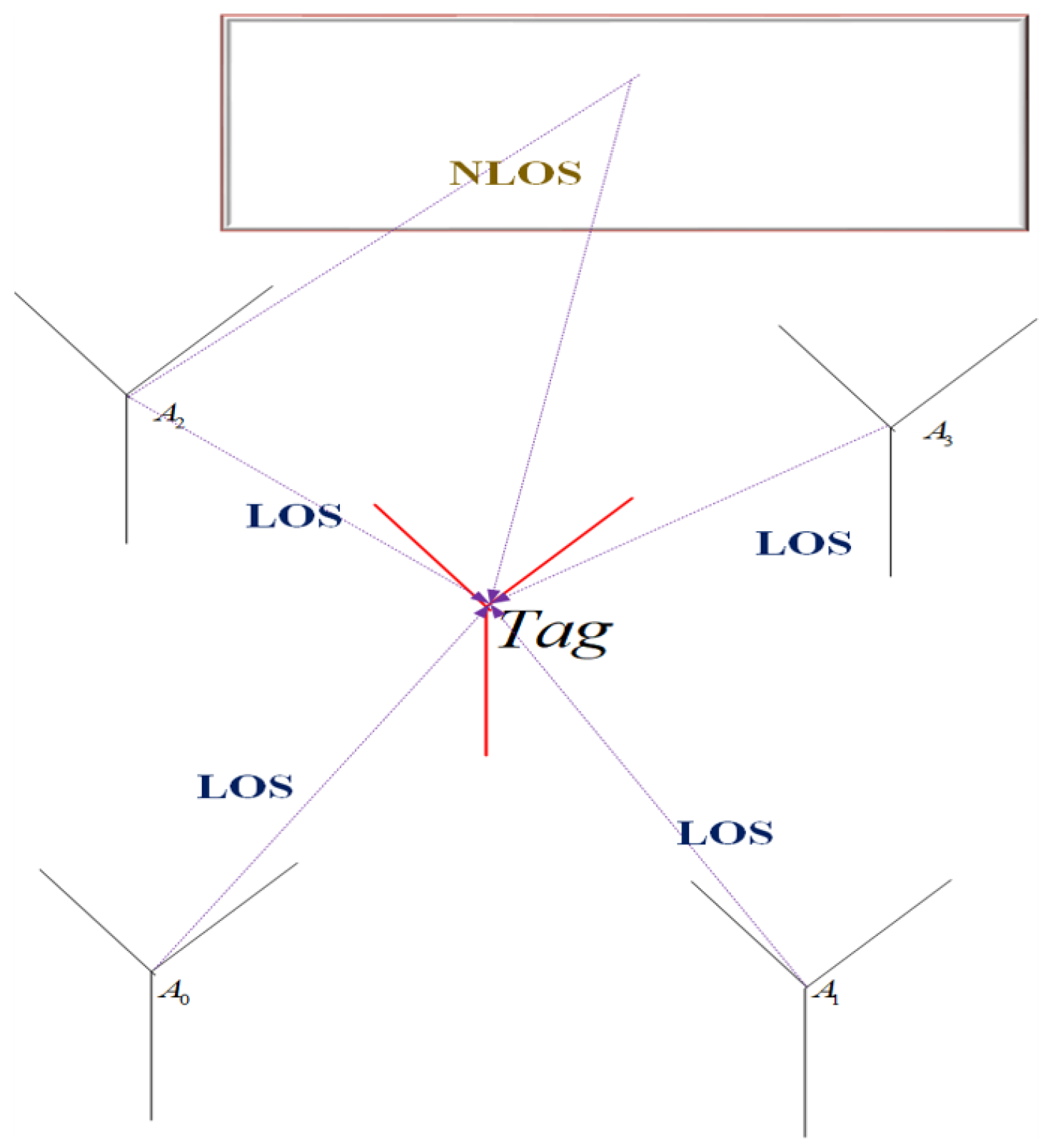
2.3. The NLOS Propogation Error Model in UWB

As indicated above, TOF ranging is performed by sending and receiving radio signals. The environment affects the propagation of radio waves in a variety of non-linear ways, including refraction, reflection, scattering, and other phenomena. The estimated distance will deviate from the real distance due to this non-linear propagation, which is known as the NLOS error. Additionally, the true linear path between nodes will not be followed by the signal propagation path. In order to fully study the pattern characteristics of anomalous data in the TOF range data set, NLOS error is briefly examined in this paper.

As seen in Figure 4, impediments prohibit radio waves from travelling in a straight path; hence, the environment used to measure distance has an effect on how NLOS mistakes happen. The typical LOS path has been blocked by the wall, resulting in a significantly longer path known as a non-LOS (NLOS) path, which is used for TOF ranging by the mobile node ($A_i$) and anchor point ($Tag$). Consequently, under NLOS situations, TOF-based range estimates are very likely to be positively skewed [30], as the first arriving multipath component travels further than the actual LOS distance. As a result, under NLOS conditions, node location estimates’ accuracy may suffer, which will materially reduce the effectiveness of the localization methods [31,32].

Due to its straightforward calculation, the Gaussian distribution model has grown to be the most-used NLOS error model, which is a major component of the classic NLOS error model. Assuming NLOS error, the following is the probability density function for the Gaussian distribution model of NLOS error:

$$f\left(e_{\mathrm{Noos}}\right)=\frac{1}{\sqrt{2\pi }\sigma }{e}^{-\frac{{\left(e_{NOS}-\mu \right)}^2}{2{\sigma }^2}}$$

(3)

where $\sigma ,\mu$ are constants.

NLOS error makes up the majority of measurement errors in UWB systems with poor communication environments, and inaccuracy in the error model will prevent the eradication of the error. Determining whether the range data contains aberrant data thus becomes a significant problem for UWB.

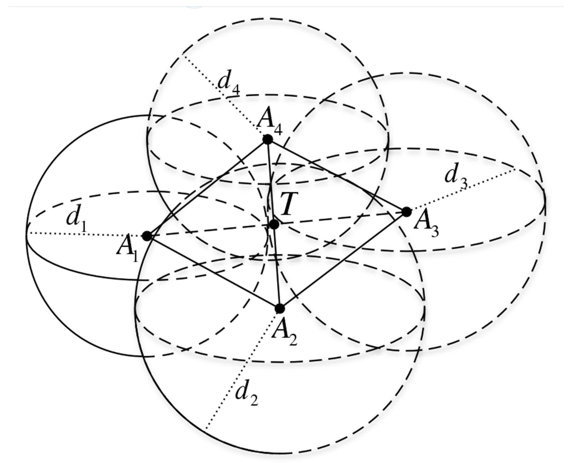
2.4. Traditional UWB Ranging Method of Quadrilateral Location Algorithm

The N edge location algorithm (N is the number of anchors) is typically used in the conventional geometric location procedure. The target node position is determined by the intersection of the radius of the measured distance between the anchor node and the target node and the centers of K anchor nodes.

Figure 5 displays the algorithm’s schematic diagram. The four anchor points are $A_i(x_{i+1},y_{i+1},z_{i+1}),(i=0,1,2,3)$, and the measured distances between them and the target Tag T are $d_1,d_2,d_3,d_4$, respectively. We calculate the target Tag’s coordinates, which are $(x,y,z)$:

$$\left\{\begin{array}{c}{(x-x_1)}^2+{(y-y_1)}^2+{(z-z_1)}^2={d_1}^2\hfill \\ {(x-x_2)}^2+{(y-y_2)}^2+{(z-z_2)}^2={d_2}^2\hfill \\ {(x-x_3)}^2+{(y-y_3)}^2+{(z-z_3)}^2={d_3}^2\hfill \\ {(x-x_4)}^2+{(y-y_4)}^2+{(z-z_4)}^2={d_4}^2\hfill \end{array}\right.$$

(4)

The coordinates of Tag are the intersection of four spheres, each with a center and radius of $A_0,A_1,A_2,A_3$, and $d_1,d_2,d_3,d_4$, respectively. Equation (4) can be solved to determine the coordinates of the target Tag as follows:

$$\left[\begin{array}{c}x\hfill \\ y\hfill \\ z\hfill \end{array}\right]=AB$$

(5)

$$A={\left[\begin{array}{ccc}2(x_1-x_4)& 2(y_1-y_4)& 2(z_1-z_4)\\ 2(x_2-x_4)& 2(y_2-y_4)& 2(z_2-z_4)\\ 2(x_3-x_4)& 2(y_3-y_4)& 2(z_3-z_4)\end{array}\right]}^{-1}$$

(6)

$$B=\left[\begin{array}{c}{x}_1^2+y_1^2+z_1^2-x_4^2-y_4^2-z_4^2+d_4^2-d_1^2\hfill \\ x_2^2+y_2^2+z_2^2-x_4^2-y_4^2-z_4^2+d_4^2-d_2^2\hfill \\ x_3^2+y_3^2+z_3^2-x_4^2-y_4^2-z_4^2+d_4^2-d_3^2\hfill \end{array}\right]$$

(7)

The calculation of the target coordinate is inaccurate when the error is substantial, especially in NLOS situations, even though such a method requires a modest computation and is simple to implement due to the influence of the distance error between the anchor points and the target point. Additionally, there is no perfect instance of several circles intersecting at one location in a practical application; as a result, this approach is not applicable.

2.5. UWB Ranging Method of Chan and Taylor Algorithm

The traditional Chan algorithm is a non-recursive method for solving a hyperbolic system of equations with high positioning precision, little computation, and a clear expression result in accordance with the function. However, its positioning accuracy will be significantly impacted if the Fresnel zone is blocked by more than 50 percent.

A recursive process known as a Taylor series expansion requires the initial estimated position of unknown nodes. By resolving the local least-squares solution of the measurement error in each iteration, it enhances the predicted position of unknown nodes. However, if the initial value is inappropriate, the method is likely to fail to converge.

In [26], the least-squares (LS) technique, Chan algorithm, and Taylor algorithm based on TDOA in UWB indoor positioning technology are evaluated and tested using dynamic and static data in an indoor line-of-sight environment, which demonstrates that the three positioning algorithms can achieve decimeter-level positioning accuracy, and the Taylor algorithm can achieve a 1-decimeter positioning accuracy. A combined location approach based on the Taylor and Chan algorithms is proposed in [27], and the design of an indoor ultra-wideband wireless location system on an FPGA development platform is finished. Both of these are based on location technology of the time difference of arrival (TDOA). In [28], the location was found using an analytical algorithm whose performance is compared to the well-known Chan’s solution, and the system concept was tested using the UWB positioning system demonstrator. Ref. [29] compares and analyzes several positioning methods, including the Taylor algorithm, Chan algorithm, and trilateration algorithm in the case of three anchors and numerous anchors, respectively.

2.6. Machine Learning-Based Ideas for UWB Localization

From a machine learning perspective, accurate localization is a process whereby a computer learns the mapping between the received range distance and the coordinates of the tag position, then generalizes the solution and gives a correction value [23]. Machine learning-based localization can be seen as a process of classifying a data set [24]: the training phase serves to train a classifier model (i.e., the localization model described above), which then primarily takes the received range distance as its input and the location coordinates of the target as its output, thus training a classifier model that meets the requirements of the task; the testing phase applies this classifier to the location estimation by feeding the collected data. In the test phase, this classifier is used for position estimation, where the collected information is input to the trained classifier and the corresponding output is the coordinates of the target point to be located, which is used as its estimated coordinates, and the coordinates are used to obtain further correction values and generate an accuracy analysis [25].

Various machine learning algorithms have been used in a wide range of applications for indoor precision positioning [33]. From the original nearest neighbor method to the successive development of Bayesian classification, SVM, and ANN, the rise of various methods has gradually improved the accuracy and usefulness of positioning methods [34]. In addition, algorithms such as clustering and feature extraction have also been applied in various segments to improve the performance of positioning algorithms [35].

2.6.1. Technology of SVM

SVMs adopt the principle of structural risk minimization to solve non-linear regression problems and can transform non-linear classification into linear classification in high-dimensional space under high-dimensional space substitution [36]. SVMs can solve problems such as classification and pattern recognition [37]. To use them to solve the difficulties in regression fitting, Vapnik introduced $\epsilon$-parameters to the SVM classification algorithm to obtain a regression-based support-vector machine (SVR) model [38]. SVR is a generalization of SVM for regression analysis and function fitting. The principle of SVR is similar to that of classification, with the only difference of introducing the concept of the loss function by SVR [39].

From the above introduction and preliminary research, it can be found that, through preliminary learning and training, the SVM-based technique can identify and distinguish NLOS signals in UWB-ranging information with high accuracy, thus achieving a more accurate classification of LOS and NLOS signals.

2.6.2. Technology of CNN

A type of feedforward neural network with a deep structure and convolutional computation is called a convolutional neural network (CNN) [40]. As one of the deep learning representative algorithms, it can classify input material that is translation-invariant according to its hierarchical structure and has the capacity for representation learning. The sparsity of interlayer connections and the parameter sharing of the convolutional kernel within the hidden layer allow CNNs to acquire grid-like topology features with little computational effort, reliable results, and no additional feature engineering needs for data [41].

A CNN is a partially connected network, with the convolution layer (denoted as conv) as its lowest layer, followed by the pooling layer (denoted as pool), and then the full connection layer (denoted as fc). For classification purposes, softmax (denoted as softmax) could be used in the last layer [42].

2.7. Assumptions

(i)

There is no other interference in the collected data other than that stated in the paper;

(ii)

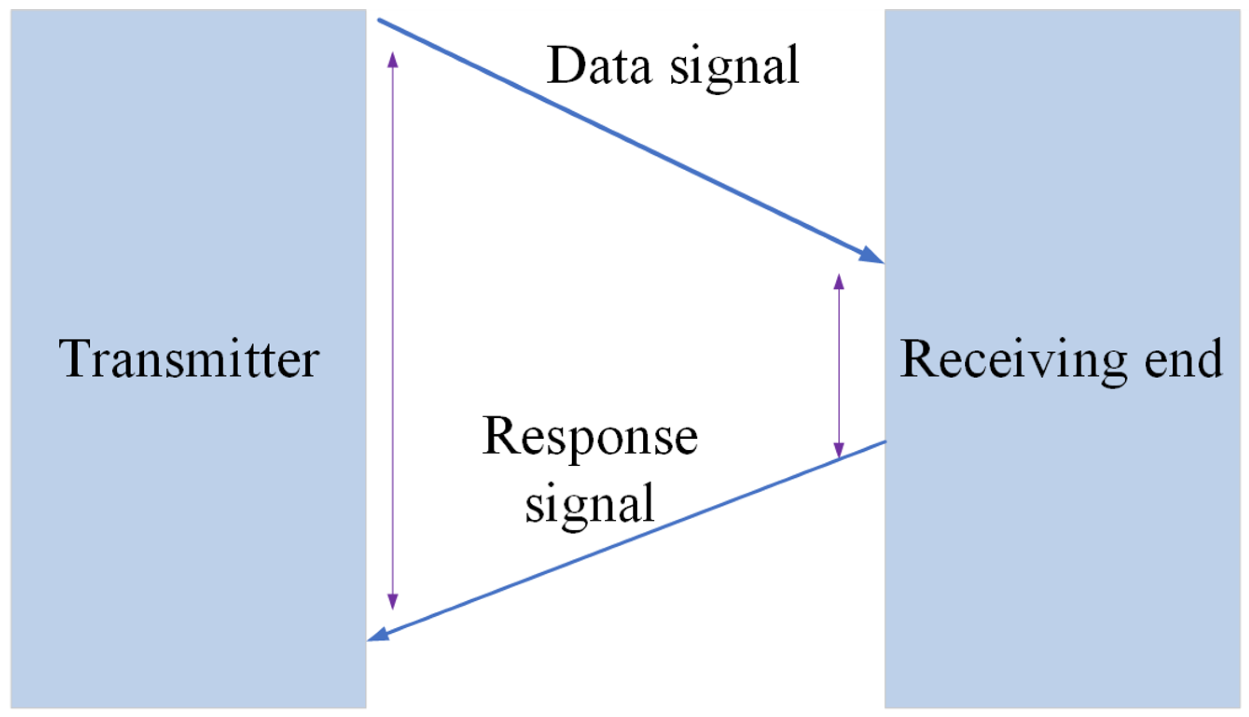
Only the TOF-based ranging principle is considered;

(iii)

It is assumed that all interferences in the experimental design are of the same prototype;

(iv)

The effect of all interferences in the experimental design on the collected data remains stable.

2.8. Notations

The main symbols used in this paper are illustrated below in

Table 1. Main symbols used in this paper.

Symbols	Description
c	The electromagnetic wave propagation speed
$T_f$	One-way flight time for TOF ranging
$A_{\mathrm{i}-1}(x_i,y_i,z_i)(i=1,2,3,4)$	Anchor point
e	Error threshold
$d\_Assemble$	Data set to be processed
$d_i(i=1,2,3,4)$	Distance measurements of anchor to target
X	Set of machine learning samples
$\Phi$	Non-linear mapping
$X_i$	Input vectors for machine learning samples
$(x,y,z)$	Coordinates of the target point to be located
$Z_p={[x,y,z]}^T$	Position of the target to be located in the hybrid weighting algorithm
$\psi$	Error vector of the hybrid weighting algorithm
Q	Covariance matrix of TOF range values
$\left(x\right(k),y(k),z(k\left)\right)$	Coordinates of the target point calculated using the kth method
$r_{i,1}\left(k\right)$	Difference between coordinates of target point to anchor point i and 1
$\Delta r$	Square of the difference between true and measured values
$\lambda \left(k\right)$	Weighting factor

.

3. Methods

3.1. Total Flow of C-T-CNN-SVM Algorithm

This study suggests a novel UWB-accurate localization algorithm based on the analysis presented above. The algorithm consists of three basic processes: an LOS/NLOS signal classification method based on SVM, an NLOS signal recognition and error elimination method based on CNN, and an accurate coordinate solution based on C-T hybrid weighting. The following section of this study refers to this innovative algorithm as the C-T-CNN-SVM algorithm, which is based on the primary procedures and techniques we use.

The fundamental steps are as follows.

(i)

Firstly, SVM-based signal classification is used to distinguish between LOS and NLOS signals. The following stage for NLOS signal detection and error eradication will use the results as input.

(ii)

Next, a CNN-based approach for recognizing and mitigating NLOS signals is proposed, which draws on the concept of neural network pattern recognition.

(iii)

Following error correction, the UWB signal data will be sent into the following hybrid weighting algorithm, which uses the Chan algorithm to calculate the initial coordinates and the Taylor algorithm to calculate the final coordinates. The specific coordinates of the target point are solved by dividing the weights of these two algorithms.

Figure 6 shows the proposed C-T-CNN-SVM algorithm’s overall processing flow diagram.

3.2. LOS/NLOS Signal Classification Based on SVM

Let X be m samples; the input vector $X_i$ is composed of l factors, and $y_i$ is the output value corresponding to $X_i$. SVM relies on nonlinear mapping $\Phi$ to map data $X_i$ to a high-dimensional feature space F, and the linear regression function established is as follows:

$$f\left(x\right)={\omega }^T\Phi \left(X_i\right)+b$$

(8)

In the above equation, $\omega$ is the weight vector of the hyperplane, while b is the offset term.

Based on the target number minimization method, the SVM regression function of LOS/NLOS signal classification can be obtained as follows:

$$\begin{array}{c}R\left(\omega \right)=min\left[\frac{1}{2}{∥\omega ∥}^2+C{\displaystyle \sum _{i=1}^l}({\xi }_i+{\xi }_i^{*})\right]\hfill \\ s.t.\left\{\begin{array}{c}{y}_i-f\left(x_i\right)\le \epsilon +{\xi }_i^{*}\hfill \\ f\left(x_i\right)-y_i\le \epsilon +{\xi }_i^{*}\hfill \\ {\xi }_i\ge 0,{\xi }_i^{*}\ge 0\hfill \end{array}\right.\hfill \end{array}$$

(9)

where ${\xi }_i$ and ${\xi }_i^{*}$ are non-negative relaxation variables, C is the punishment factor, and $\epsilon$ is the insensitive loss function parameter.

Using the Lagrange method to solve the optimal solution problem, the above formula is converted into the dual form, as follows:

$$\begin{array}{c}J(a_i,a_i^{*})=max\left[\frac{1}{2}{\displaystyle \sum _{i=1}^l}{\displaystyle \sum _{j=1}^l}(a_i-a_i^{*})(a_j-a_j^{*})K(x_i,x_j)-{\displaystyle \sum _{i=1}^l}(a_i+a_i^{*})\epsilon +{\displaystyle \sum _{i=1}^l}(a_i-a_i^{*})y_i\right]\hfill \\ s.t.\left\{\begin{array}{c}{\displaystyle \sum _{i=1}^l}(a_i-a_i^{*})=0\hfill \\ 0\le a_i,a_i^{*}\le C\hfill \end{array}\right.\hfill \end{array}$$

(10)

where $a_i$ and $a_i^{*}$ are Lagrange coefficients.

Thus, the final SVM regression function for LOS/NLOS signal classification can be written as follows:

$$f\left(x\right)=\sum _{i=1}^l(a_i-a_i^{*})K(x_i,x)+b^{*}$$

(11)

In the above equation, $a_i$ and $a_i^{*}$ are Lagrange coefficients, and $b^{*}$ is the optimized bias term. The kernel function $K(x_i,x)$ adopts the radial basis function (RBF) as follows:

$$K(x_i,x)=exp(-g{\left|x_i-x\right|}^2)$$

(12)

where g is the parameter width of the kernel function.

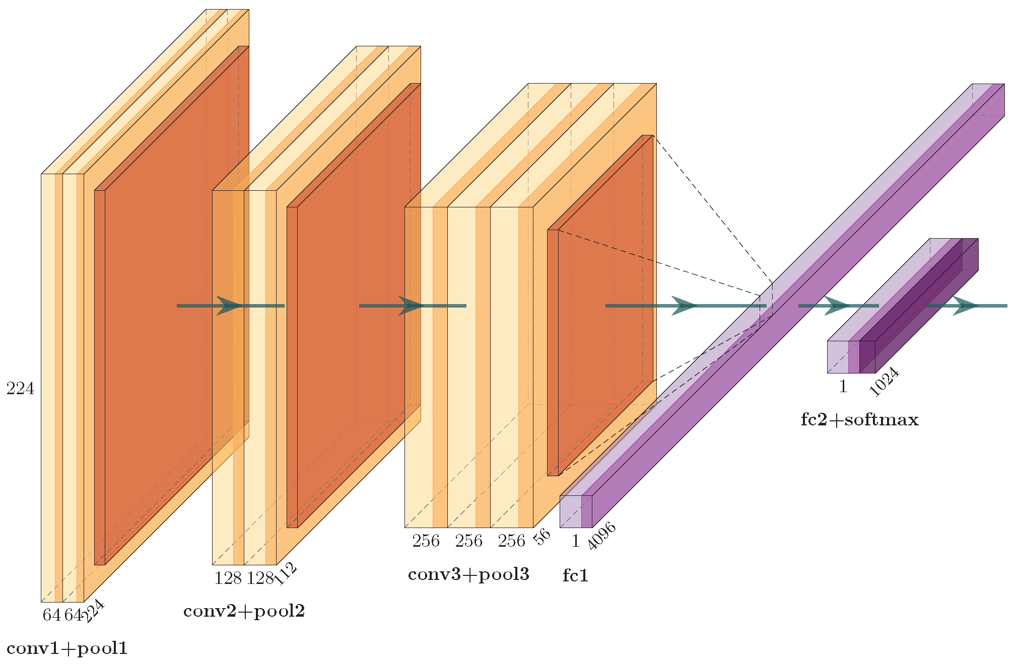
3.3. CNN-Based Method for NLOS Signal Recognition and Error Elimination

NLOS signal recognition and error removal will be accomplished in this paper using a convolutional neural network (CNN). Our CNN will first adequately learn data sets of recognized UWB signal patterns (known as LOS, NLOS, and mixed NLOS-LOS). Following training, the CNN will identify patterns in the input data set utilized for precise UWB positioning before performing error reduction.

The CNN in Figure 7 will choose the data, build and train the networks, and assess the effectiveness of pattern recognition using cross-entropy and the obfuscation matrix. The two-layer feedforward network (Patternnet), which is used in this method, has sigmoid hidden neurons and softmax output neurons. The proportional conjugate gradient back propagation function will train the neural network.

3.3.1. NLOS Signal Recognition

The algorithm used by the CNN to detect anomalies primarily consists of four stages: data preparation, model training, multi-step prediction classification, and performance evaluation. The following diagram illustrates the precise methodology of our CNN-based NLOS signal recognition.

Step 1: Selection of training and recognition data sets.

Step 2: Setting up the training, validation, and test data sets.

Step 3: Building a neural network.

The number of neurons in the hidden layer is calculated using the equation below.

$$N_h=\frac{N_S}{\alpha \left(N_i+N_o\right)}$$

(13)

where $N_i$, $N_o$, and $N_S$ are the number of neurons in the input or output layer and the number of samples in the training set, respectively; $\alpha$ is an arbitrary value variable with a range of 2 to 10.

Step 4: Training neural networks.

Step 5: Evaluation of the neural network.

Step 6: Recognizing NLOS signal patterns for target data sets.

3.3.2. NLOS Error Mitigation

The NLOS range error can be predicted using the parameters provided by the neural network modules combined with the range estimates, according to several earlier studies [43,44]. Then, NLOS error mitigation can be carried out using the expected range error. An investigation of the permutation importance and the significance of each input parameter that influences the accuracy of the prediction error using an ANN is shown in [43]. This inspired us to conduct related research, and the results were as follows: the main influences on the prediction error are range measurements, maxNoise, stdNoise, and rangeError. Since the aforementioned four traits account for more than 80 percent of all characteristics, we will just concentrate on these four characteristics in this research.

Figure 8 shows the error histograms of the entire validation data set for three different situations as an illustration of the impact of NLOS error mitigation. Range errors before the CNN application are represented in blue, while the range and maxNoise errors following CNN output correction are represented in orange, and range errors following correction based on all previously specified input parameters are represented in yellow. The error prediction is found to reduce the bias and the standard deviation of the errors. The standard deviation decreases from 13.65 cm to 4.35 cm, while the mean error decreases from 3.65 cm to 0.27 cm. After this mistake correction, the errors are practically distributed normally.

The data shown above clearly demonstrate that after training a CNN for NLOS recognition and performing NLOS mitigation, the accuracy of UWB range measurements may be greatly increased.

3.4. Final Accurate UWB Coordinate Solution Based on Hybrid Weighting of Chan and Taylor Algorithm

This module will receive the UWB signal data set after NLOS recognition and error removal to provide the precise coordinate solution. According to the analysis of UWB signal data sets with NLOS conducted above above, using just the single Chan or Taylor algorithm for processing will eventually result in a significant mistake in the target coordinates.

The Chan method is therefore used in this study as the initial algorithm for positioning to produce a relatively accurate initial solution coordinate of anchor points and to simplify the convergence of the Taylor algorithm, thereby reducing the complexity of the operation and increasing operational efficiency. The hybrid weighted localization approach based on the Chan–Taylor method is employed on this basis. To achieve more precise location coordinates, such a solution will make full use of the strengths of these two methods and combine them successfully.

3.4.1. Target Coordinate Preliminary Solution Using Chan Algorithm

The three-dimensional positioning model based on the Chan algorithm will be used in this work to initially determine the placement of anchor points. The precise procedure is illustrated as follows:

Step 1

The expression for the distance $r_i$ between the target and anchor is:

$$r_i=\sqrt{{(x_i-x)}^2+{(y_i-y)}^2+{(z_i-z)}^2}$$

(14)

We square both sides, then obtain:

$$\begin{array}{c}{r_i}^2={(x_i-x)}^2+{(y_i-y)}^2+{(z_i-z)}^2\hfill \\ =K_i-2x_{i}x-2y_{i}y-2z_{i}z+x^2+y^2+z^2\hfill \end{array}$$

(15)

where $K_i={x_i}^2+{y_i}^2+{z_i}^2(i=1,2,3,4)$.

Allow $r_{i,1}$ to stand for the difference between the target’s distance from the i-th anchor and its distance from the l-th anchor:

$$\begin{array}{c}{r}_{i,1}=r_i-r_1=\sqrt{{(x_i-x)}^2+{(y_i-y)}^2+{(z_i-z)}^2}\hfill \\ -\sqrt{{(x_1-x)}^2+{(y_1-y)}^2+{(z_1-z)}^2}\hfill \end{array}$$

(16)

Let $i=1$; then, $r_{i,1}=0$. Therefore, Equation (16) can be expressed simply as:

$$r_{i,1}^2+2r_{i,1}{r}_1=K_i-2x_{i,1}x-2y_{i,1}y-2z_{i,1}z-K_1$$

(17)

The above equation is a nonlinear system of equations, where $x_{i,1}=x_i-x_1,y_{i,1}=y_i-y_1,z_{i,1}=z_i-z_1$, $x,y,z,r_1$ are unknowns.

Step 2

Let $Z_p={[x,y]}^T$ be the desired target position and $Z_a={[{Z_p}^T,R_1]}^T$ be the unknown vector. Then, we obtain the following as the error vector:

$$\psi =h-G_a{Z}_a^0$$

(18)

Among them:

$$h=\frac{1}{2}\left[\begin{array}{c}{R}_{2,1}^2-K_2+K_1\\ R_{3,1}^2-K_3+K_1\\ ⋮\\ R_{M,1}^2-K_M+K_1\end{array}\right],(M=4)$$

(19)

$$G_a=\left[\begin{array}{ccc}{\mathrm{x}}_{2,1}& {\mathrm{y}}_{2,1}& R_{2,1}\\ {\mathrm{x}}_{3,1}& {\mathrm{y}}_{3,1}& R_{3,1}\\ & ⋮& \\ {\mathrm{x}}_{M,1}& {\mathrm{y}}_{M,1}& R_{M,1}\end{array}\right],(M=4)$$

(20)

The error vector can be obtained as follows:

$$\psi =cBn+0.5c^{2}n\otimes n$$

(21)

where ⊗ is the usual inner product of Euclidean space and $B=diag\{R_2^0,R_3^0,R_4^0\}$. Equation (21)’s final term can be removed because $cn<<R_{i,1}^0$, and the vector difference between the ideal error-free reference signal and the actual transmitted signal at a specific moment is roughly a random vector with a normal distribution, with its covariance being:

$$\Psi =E\left[\psi {\psi }^T\right]=c^{2}BQB$$

(22)

where $\mathrm{Q}=\mathrm{E}\left[\mathrm{nn}\right]$, and the approximate solution of (11) obtained by the least square method is:

$$\begin{array}{c}Za=argmin\left\{{\left(h-G_a{Z}_a\right)}^T{\Psi }^{-1}\left(h-G_a{Z}_a\right)\right\}\hfill \\ ={\left(G_a^T{\Psi }^{-1}{G}_a\right)}^{-1}{G}_a^T{\Psi }^{-1}h\hfill \end{array}$$

(23)

If the distance between the target point and the anchor point is far, $B\approx R_{}^{0}I$, then the above equation can be replaced by:

$$Z_a={\left(G_a^T{Q}^{-1}{G}_a\right)}^{-1}{G}_a^T{Q}^{-1}h$$

(24)

The target point’s coordinates, $(\mathrm{x},\mathrm{y},\mathrm{z})$, may be found from $Z_a$. Thus, the Chan algorithm-based preliminary solution of the target coordinates is finished.

3.4.2. Taylor Series-Based Technique for the Accurate Coordinate Solution of the Anchor Point

The target node’s initial position must be estimated when using the Taylor series expansion method, which necessitates assigning the initial value (results solved by the Chan algorithm). The ideal iteration value is then derived after calculating the local solution using the least-squares approach. The output of the positioning information depends on whether the error of the unknown node position and coordinate falls within the threshold value.

A specific function, $f_i\left(x,y,z,x_i,y_i,z_i\right)$, can be used to illustrate the relationship between anchor points and characteristic signals. The following prerequisite needs to be satisfied if the threshold value is represented by $\eta$.

$$\left|\Delta x+\Delta y\right|<\eta$$

(25)

Consider that the initial value of the anchor point coordinates that the solution yields is $(x_0,y_0,z_0)$, and $x=x_0+\Delta x,y=y_0+\Delta y,z=z_0+\Delta z$. The formula’s greater-than-two elements are not taken into account as $f_i\left(x,y,z,x_i,y_i,z_i\right)$ at $(x_0,y_0,z_0)$ undergoes the Taylor series expansion. The outcomes will then be as follows:

$$\begin{array}{c}{f}_i\left(x,y,z,x_i,y_i,z_i\right)=f_i\left(x_0,y_0,z_0,x_i,y_i,z_i\right)+\hfill \\ \left(\Delta x\frac{\partial }{\partial x}+\Delta y\frac{\partial }{\partial y}+\Delta z\frac{\partial }{\partial z}\right)f_i\left(x_0,y_0,z_0,x_i,y_i,z_i\right)\hfill \end{array}$$

(26)

Therefore, the error vector $\psi$ can be obtained as:

$$\psi =h_i-G_i\delta$$

(27)

Among them are:

$$h_i=\left[\begin{array}{c}{r}_{2,1}-\left(r_2-r_1\right)\\ r_{3,1}-\left(r_3-r_1\right)\\ ⋮\\ r_{L,1}-\left(r_L-r_1\right)\end{array}\right]$$

(28)

$$\delta =\left[\begin{array}{c}\Delta x\hfill \\ \Delta y\hfill \end{array}\right]$$

(29)

$$G_i=\left(\begin{array}{ccc}\frac{x_1-x}{r_1}-\frac{x_2-x}{r_2}& \frac{y_1-y}{r_1}-\frac{y_2-y}{r_2}& \frac{z_1-z}{r_1}-\frac{z_2-z}{r_2}\\ \frac{x_1-x}{r_1}-\frac{x_3-x}{r_3}& \frac{y_1-y}{r_1}-\frac{y_3-y}{r_3}& \frac{z_1-z}{r_1}-\frac{z_3-z}{r_3}\\ ⋮& ⋮& ⋮\\ \frac{x_1-x}{r_1}-\frac{x_L-x}{r_L}& \frac{y_1-y}{r_1}-\frac{y_L-y}{r_L}& \frac{z_1-z}{r_1}-\frac{z_L-z}{r_L}\end{array}\right)$$

(30)

The distance between the anchor node and the unknown node throughout an iteration is denoted by $r_i(i=1,2,3,4)$. Equation (28)’s weighted least-squares answer is:

$$\delta =\left[\begin{array}{c}\Delta x\hfill \\ \Delta y\hfill \end{array}\right]={\left(G_i^T{Q}^{-1}{G}_i\right)}^{-1}{G}_i^T{Q}^{-1}{h}_i$$

(31)

The covariance matrix of the TOF ranging value is represented by Q in the equation above. When the calculation procedure is complete, the calculation result at this point is the anchor point’s final positioning coordinate, and the computation is complete if the calculation result of $\delta$ is included in the previously stated threshold value $\eta$. Thus, the more accurate coordinate value of the anchor point based on the Taylor series algorithm is accomplished.

3.4.3. Final Determination of Anchor Coordinates Based on Chan–Taylor Mixed Weighting Method

Using the kth approach, we define $\left(x\right(k),y(k\left)\right)$ as the target’s coordinates ($k=1$ is the Chan algorithm, and $k=2$ is the Taylor series algorithm), and define $r_{i,1}\left(k\right)$ as the distance difference:

$$\begin{array}{c}{r}_{i,1}\left(k\right)=\sqrt{{[x\left(k\right)-x_i]}^2+{[y\left(k\right)-y_i]}^2+{[z\left(k\right)-z_i]}^2}\hfill \\ -\sqrt{{[x\left(k\right)-x_1]}^2+{[y\left(k\right)-y_1]}^2+{[z\left(k\right)-z_1]}^2}\hfill \end{array}$$

(32)

We define $\Delta r$ as the square of the difference between the true value and the measured value:

$$\Delta r={[r_{i,1}-r_{i,1}\left(k\right)]}^2$$

(33)

The weighting coefficient $\lambda \left(k\right)$ is defined as:

$$\lambda \left(k\right)=\frac{{\displaystyle \sum _{i=2}^4}\Delta r}{4}$$

(34)

The algorithm shows that the estimation is more accurate the smaller $\Delta r$ is. As a result, the estimated position coordinates are more precise the smaller the weighting coefficient $\lambda \left(k\right)$ is, which implies that a higher fraction of the measured data acquired by this positioning approach should be accounted for. Finally, the target’s precise coordinates are as follows:

$$x=\frac{{\displaystyle \sum _{k=1}^k}\frac{x\left(k\right)}{\lambda \left(k\right)}}{{\displaystyle \sum _{k=1}^k}\frac{1}{\lambda \left(k\right)}},y=\frac{{\displaystyle \sum _{k=1}^k}\frac{y\left(k\right)}{\lambda \left(k\right)}}{{\displaystyle \sum _{k=1}^k}\frac{1}{\lambda \left(k\right)}},z=\frac{{\displaystyle \sum _{k=1}^k}\frac{z\left(k\right)}{\lambda \left(k\right)}}{{\displaystyle \sum _{k=1}^k}\frac{1}{\lambda \left(k\right)}}$$

(35)

Thus, the accurate coordinate solution based on the C-T hybrid weighting algorithm is finally determined.

4. Experiment and Analysis

To sufficiently show the usefulness of the final coordinate precise location method based on a Chan–Taylor hybrid algorithm, an NLOS recognition and error reduction method based on CNN, and an LOS/NLOS classification method based on SVM, the proposed algorithm (C-T-CNN-SVM) was compared with the enhanced algorithms and classic algorithms, which included the hybrid Chan–Taylor algorithm (C-T), the hybrid Chan–Taylor–CNN algorithm (C-T-CNN), the Chan algorithm, the Taylor algorithm, and the quadrangle-intersection algorithm. The evaluation indices of range error based on TOF are thoroughly researched in the context of the data set provided in this work.

The total number of 648 data sets used varied in terms of the number of LOS and NLOS signals. The testing environment used MATLAB 2019A, an Intel i7 processor, and a TELESLA GPU V100.

4.1. Analysis of NLOS Mitigation Performance

As has been stated, NLOS mitigation is one of the most significant perspectives to deal with NLOS errors in UWB positioning issues, which also becomes an important index to test the effectiveness of the proposed method. Considering this, in the simulation part, we will first conduct the comparison of NLOS mitigation performance between the proposed C-T-CNN-SVM algorithm and some of the state-of-the-art algorithms, which have been analyzed in the introduction. For simplicity of analysis, we call the algorithms in [34,35,36] LED mitigation, SPGP mitigation, and SLAT mitigation, respectively. For comparison, the proposed method is called C-T-CNN-SVM mitigation.

As can be seen in Figure 9, compared with other state-of-the-art algorithms, the proposed C-T-SVM-CNN algorithm maintains the lowest level of RMSE of NLOS mitigation error with the increase in the distance measurement error. Even with a distance measurement error of 50 cm, the RMSE of C-T-SVM-CNN is 47.5 cm. By comparison, the RMSE of the LED mitigation, SPGP mitigation, and SLAT mitigation are as high as 61.4 cm, 67.9 cm, and 74.2 cm.

4.2. Accuracy Analysis of the Algorithms

The experiment involved solving the target coordinates using the suggested C-T-CNN-SVM technique and comparing the outcomes to the reference values provided for the target coordinates. We determined the precise coordinates of 648 targets using the technique described in this research, and we compared the positioning model’s 3-dimensional $(x,y,z)$ accuracy, 2-dimensional $(x,y)$ accuracy, and 1-dimensional accuracy. Below are the detailed outcomes.

4.2.1. 1D Accuracy Analysis of the Algorithms

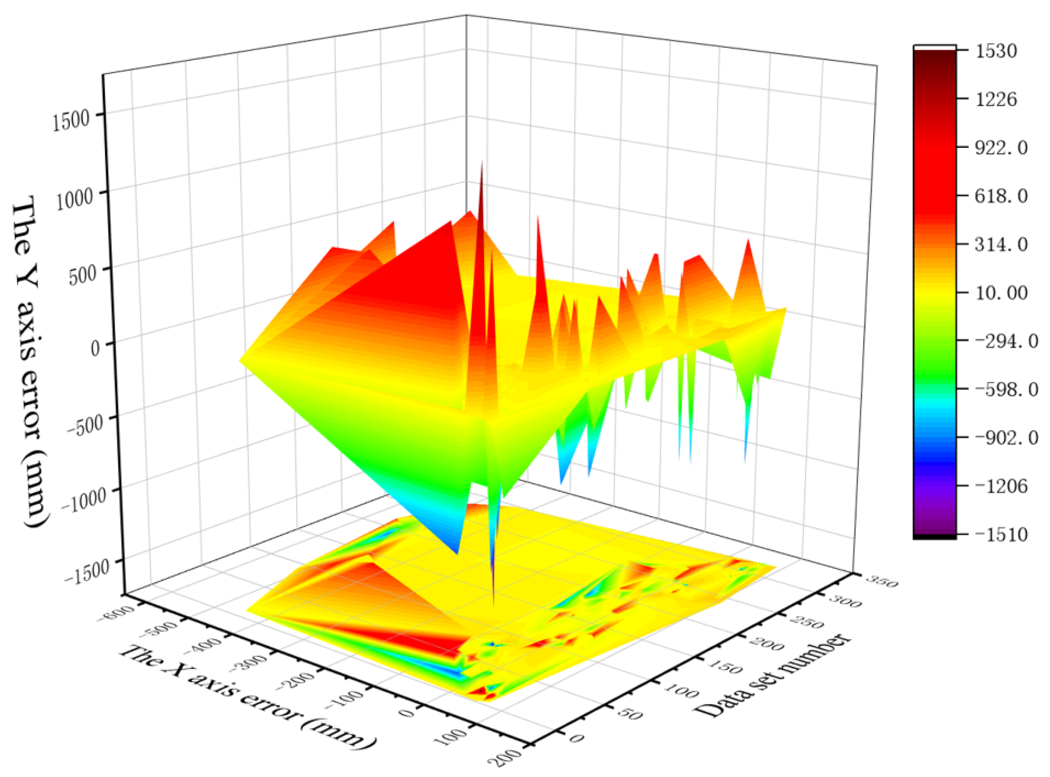
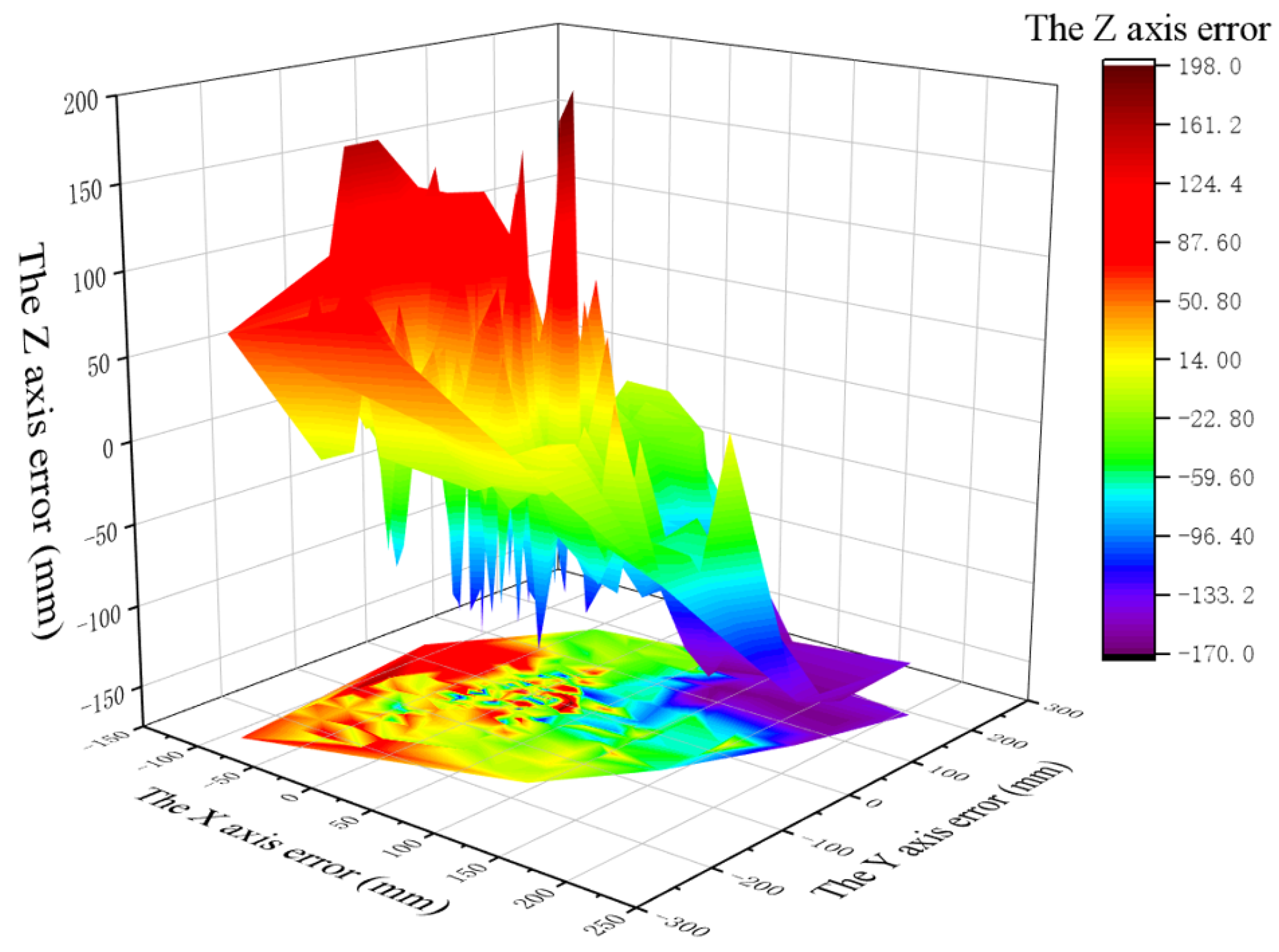
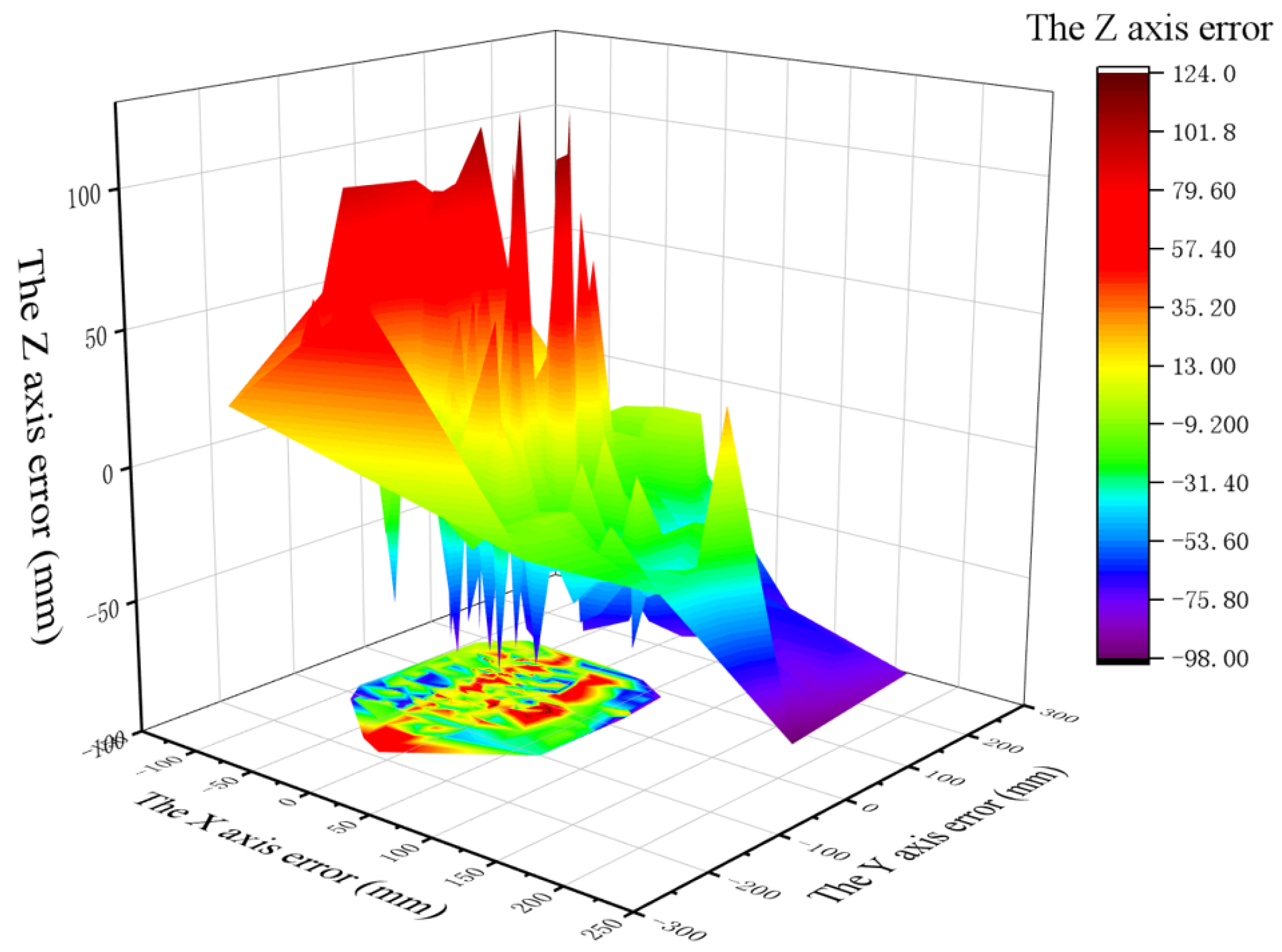
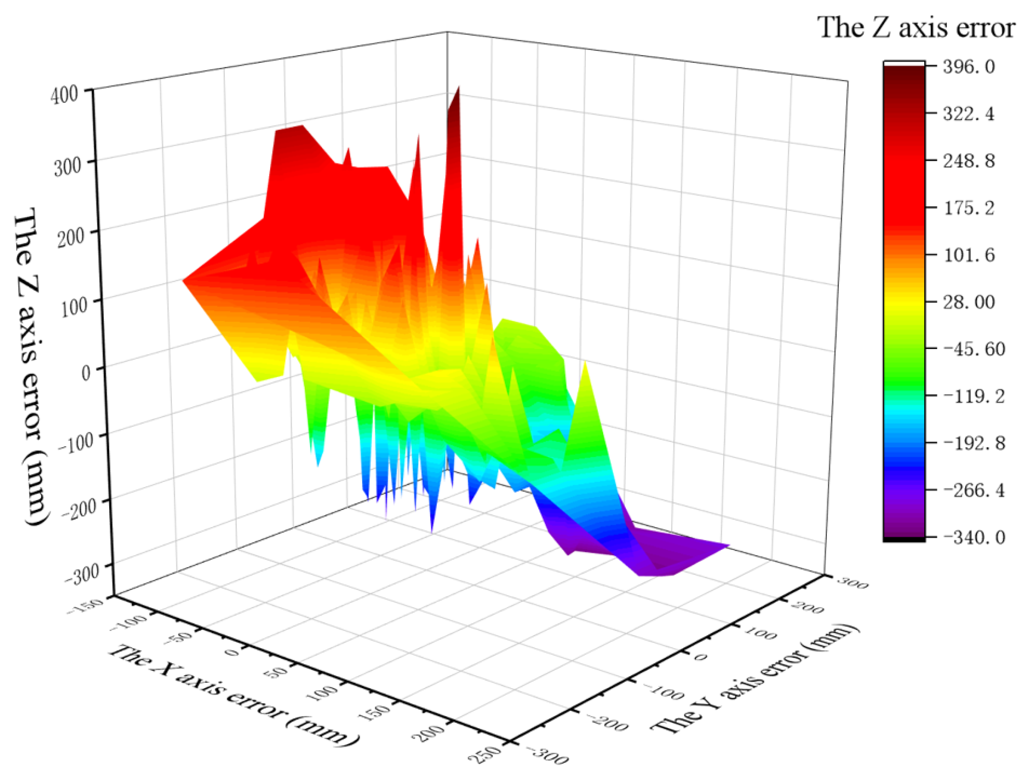
To fully illustrate the superiority of the positioning model in this paper, the traditional spatial intersection model and the C-T-CNN-SVM model proposed in this paper were used to solve the normal data set and abnormal data set respectively. The one-dimensional error results of normal and abnormal data sets using the C-T-CNN-SVM method and the traditional intersection method are compared and analyzed in Figure 10.

(i)

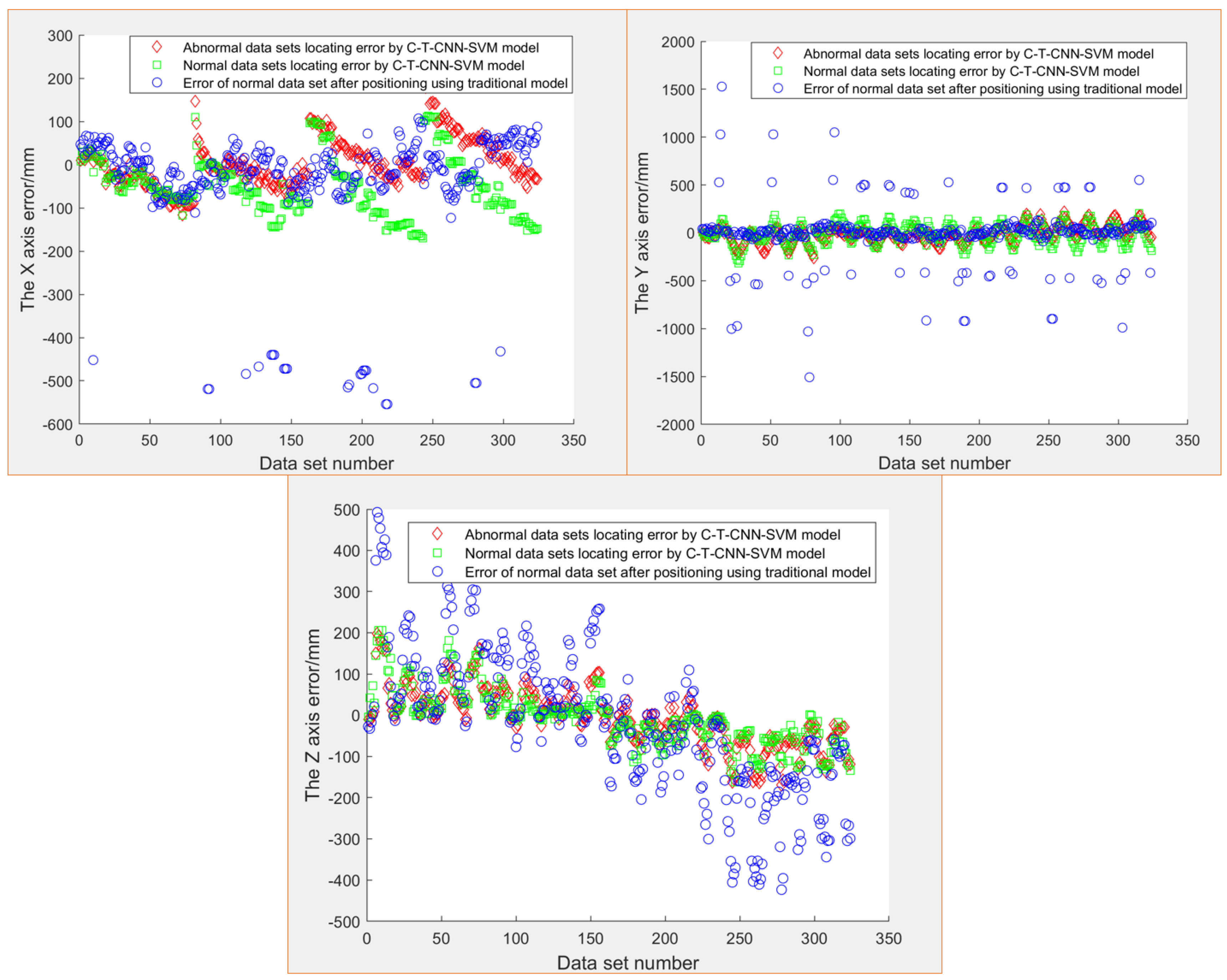
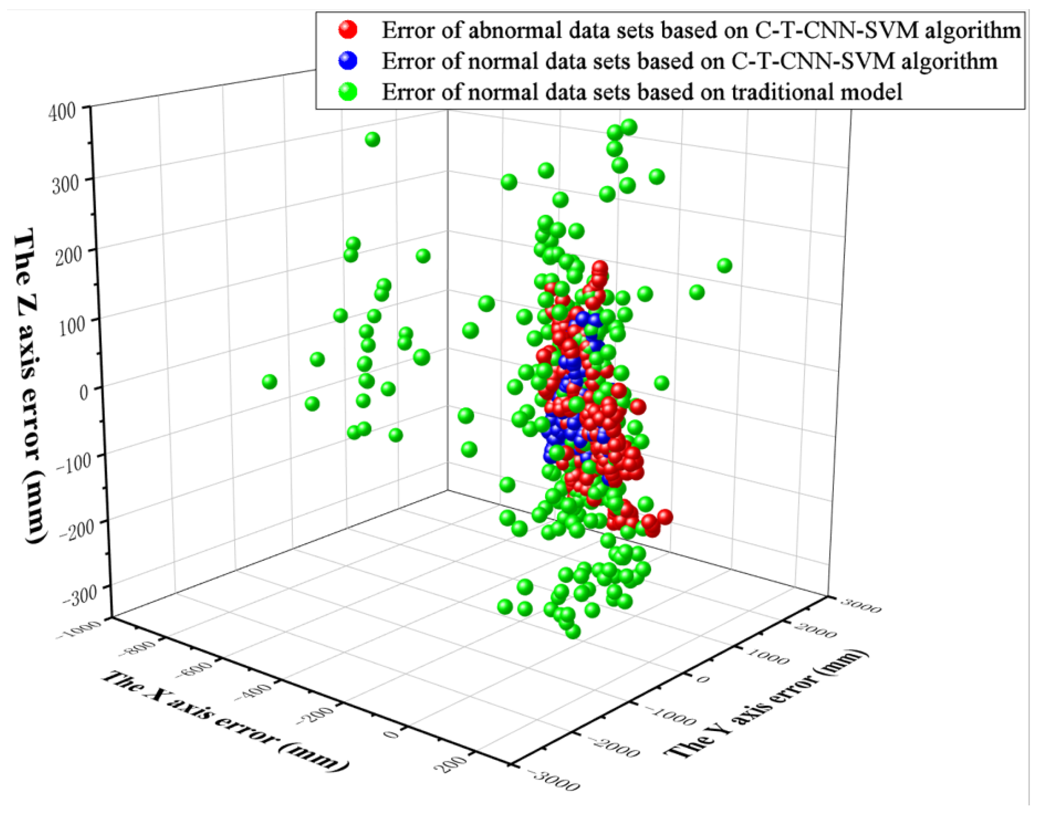
It can be seen from Figure 10 that, under the model in this paper, the one-dimensional error after target positioning is within 175 mm on the X-axis and Y-axis. The X-axis error of normal data sets is generally less than 60 mm, and the Y-axis error is generally less than 75 mm. The error of the X-axis and Y-axis of an abnormal data set is generally less than 100 mm. The Z-axis error is larger than that of the X-axis and Y-axis, but generally less than 200 mm.

(ii)

For comparison, although the coordinate error obtained by the traditional model is within 200 mm under most data sets, it has an abnormal error as high as 600 mm. In terms of Y-axis error, compared with the C-T-CNN-SVM model, although the error of the traditional model is within 500 mm under most data sets, there exists an abnormal result of 1000 mm. In terms of Z-axis error, the coordinate errors obtained by the traditional model are all within 200 mm under most data sets, though there remains an error of 500 mm.

The above one-dimensional comparison results fully demonstrate that the accuracy effect of this model is superior in one dimension, which can adequately meet the target location problem in both normal and abnormal environments.

4.2.2. 2D Accuracy Analysis of the Algorithms

Figure 11, Figure 12 and Figure 13 show the comparison results of the two-dimensional error of the target location based on abnormal and normal data sets of the proposed model and traditional model.

As can be seen from Figure 11, Figure 12 and Figure 13, the model in this paper can ensure that the errors of the X and Y axes are generally within 200 mm even in the abnormal data set, which could fully meet the relevant requirements for accurate positioning of UWB. By contrast, the traditional positioning model still has a positioning error of up to 500 mm even in the two-dimensional case. The above analysis proves that the precise positioning model in this paper still has high accuracy in two dimensions.

4.2.3. 3D Accuracy Analysis of the Algorithms

Meanwhile, based on the target coordinates obtained by the solution, the 3D $(X,Y,Z)$ accuracy of the positioning model was analyzed, and the specific results are shown in Figure 14, Figure 15, Figure 16 and Figure 17.

It can be seen from Figure 14, Figure 15, Figure 16 and Figure 17 that the positioning errors of the 3D coordinates of the target located by the model in this paper are all within 200 mm, and most of the positioning errors fall within (100 mm, 100 mm, 100 mm). As a comparison, the 3D error of the traditional positioning model is obviously larger, and most of the errors fall outside (100 mm, 200 mm, 200 mm), which fully demonstrates the superiority of the positioning model in this paper in 3D positioning.

4.3. Validity Analysis of the Algorithms

Furthermore, in order to further analyze the superiority of the algorithm adopted in this paper, the C-T-CNN-SVM algorithm is compared with the error of the traditional Chan algorithm, Taylor algorithm, and intersection algorithm. The main indicators are the cumulative error probability (CDF) and root-mean-square difference (RMSE). The details are as follows.

4.3.1. Cumulative Error Probability Analysis of the Algorithms

As can be seen from Figure 18, the CDF of the proposed algorithm grows slowest as the location error increases. When the location error is less than 10 cm, the CDF of the proposed algorithm only reaches $0.17$, while for comparison, the CDF of the four-side intersection algorithm is as high as $0.85$. When the positioning error reaches 30 cm, only the CDF of the proposed algorithm remains in an acceptable range, which fully demonstrates the superiority of the proposed algorithm.

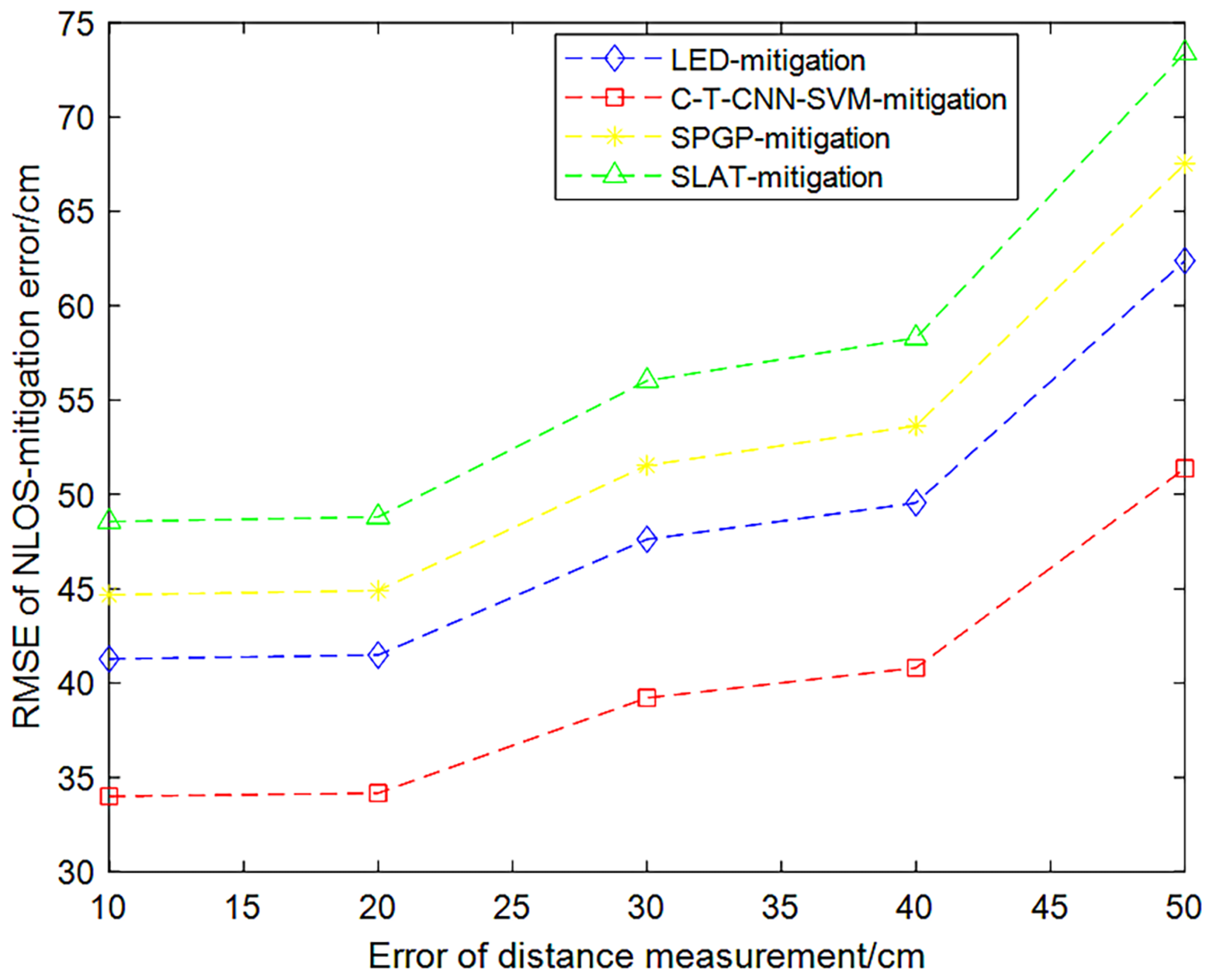
4.3.2. Root-Mean-Square Difference Analysis of the Algorithms

Figure 19 shows the curve of the root-mean-square error (RMSE) distribution and distance error of each algorithm. It can be seen from the figure that when the distance error is less than 30 cm, the RMSE of the other three algorithms except the quadrilateral intersection algorithm is in an acceptable range. However, when the distance error is greater than 30 cm, only the RMSE of the proposed algorithm is ideal. By contrast, when the distance error is 10 cm, the RMSE of the quadrilateral intersection positioning algorithm is already very large.

4.4. Complexity Analysis of the Proposed Algorithm

In this paper, we perform a complexity analysis on the C-T-CNN-SVM algorithm proposed in this paper using the following indicator [29,45]: time complexity, (also known as the amount of computations), which is denoted by time and expressed in FLOPs. It represents the number of model operations, also known as floating-point operations, which determines the model’s training or prediction time. The specific expression is as follows:

$$Time\left(\sum _{l=1}^D{M}_l^2·K_l^2·C_{l-1}·C_l\right)$$

(36)

where D is the number of convolutional layers possessed by the neural network; L is the lth convolution layer of the neural network; $C_l$ is the number of output channels of the lth convolutional layer; K is the side length of each convolution kernel; and M is the side length of the output feature graph of each convolution kernel, and it is determined by four parameters: input matrix size X, convolution kernel size K, padding and stride. The specific expression of M is as follows:

$$M=(X-K+2·Padding)/Stride+1$$

(37)

Using the above indicator, this paper analyzes the complexity of the C-T-SVM-CNN algorithm proposed in this paper. The result of each part of C-T-SVM-CNN is also listed, as shown in

Table 2. Complexity analysis of the proposed algorithm.

	SVM	CNN	C-T	C-T-CNN-SVM
Time (FLOPS)	20 G	133.4 G	15 G	168.4 G

.

The above experiments fully prove the effectiveness, accuracy and superiority of the proposed C-T-CNN-SVM algorithm, which will play an important role in UWB indoor positioning under strong interference in the future.

5. Conclusions

In this paper, using the idea of SVM and neural network pattern recognition, the classification, recognition and mitigation of NLOS signals based on SVM and CNN are proposed. On this foundation, the UWB signal data that have undergone error correction are fed into the next hybrid weighting process. The precise coordinates of the target point are resolved by allocating the weights of the Chan and Taylor algorithms. The C-T-CNN-SVM method is then evaluated and verified using the measured data, demonstrating its validity and accuracy. In order to meet the growing need for wireless indoor locating and communication, further research might concentrate on the practical deployment of such an algorithm.

References

1. Kok, M.; Hol, J.D.; Schon, T.B. Indoor Positioning Using Ultrawideband and Inertial Measurements. IEEE Trans. Veh. Technol. 2015, 64, 1293–1303. [Google Scholar] [CrossRef] [Green Version]
2. Choi, J.W.; Quan, X.; Cho, S.H. Bi-Directional Passing People Counting System Based on IR-UWB Radar Sensors. IEEE Internet Things J. 2017, 5, 512–522. [Google Scholar] [CrossRef]
3. Ahmed, S.; Wang, D.; Park, J.; Cho, S.H. UWB-gestures, a public dataset of dynamic hand gestures acquired using impulse radar sensors. Sci. Data 2021, 8, 1–9. [Google Scholar] [CrossRef] [PubMed]
4. Tiemann, J.; Pillmann, J.; Wietfeld, C. Ultra-Wideband Antenna-Induced Error Prediction Using Deep Learning on Channel Response Data. IEEE Veh. Technol. Conf. 2017. [Google Scholar] [CrossRef]
5. Choliz, J.; Eguizabal, M.; Hernandez-Solana, A.; Valdovinos, A. Comparison of algorithms for uwb indoor location and tracking systems. In Proceedings of the 2011 IEEE 73rd Vehicular Technology Conference (VTC Spring), Budapest, Hungary, 15–18 May 2011; pp. 1–5. [Google Scholar] [CrossRef]
6. Liu, F.; Zhang, J.; Wang, J.; Han, H.; Yang, D. An UWB/Vision Fusion Scheme for Determining Pedestrians’ Indoor Location. Sensors 2020, 20, 1139. [Google Scholar] [CrossRef] [Green Version]
7. Shi, G.; Ming, Y. Survey of Indoor Positioning Systems Based on Ultra-wideband (UWB) Technology. In Wireless Communications, Networking and Applications; Lecture Notes in Electrical Engineering; Springer: New Delhi, India, 2015; pp. 1269–1278. [Google Scholar] [CrossRef]
8. Liu, F.; Li, X.; Wang, J.; Zhang, J. An Adaptive UWB/MEMS-IMU Complementary Kalman Filter for Indoor Location in NLOS Environment. Remote. Sens. 2019, 11, 2628. [Google Scholar] [CrossRef] [Green Version]
9. Guvenc, I.; Chong, C.-C. A survey on TOA based wireless localization and NLOS mitigation techniques. IEEE Commun. Surv. Tuts. 2009, 11, 107–124. [Google Scholar] [CrossRef]
10. Guvenc, C.-C.; Chong, C.C.; Watanabe, F.; Inamura, H. NLOS identification and weighted least-squares localization for UWB systems using multipath channel statistics. EURASIP J. Adv. Signal Process. 2008, 36, 271984. [Google Scholar]
11. Li, X.; Cai, X.; Hei, Y.; Yuan, R. NLOS identification and mitigation based on channel state information for indoor WiFi localisation. IET Commun. 2017, 11, 531–537. [Google Scholar] [CrossRef]
12. Marano, S.; Gifford, W.M.; Wymeersch, H.; Win, M.Z. NLOS identification and mitigation for localization based on UWB experimental data. IEEE J. Sel. Areas Commun. 2010, 28, 1026–1035. [Google Scholar] [CrossRef] [Green Version]
13. Wymeersch, H.; Marano, S.; Gifford, W.M.; Win, M.Z. A Machine Learning Approach to Ranging Error Mitigation for UWB Localization. IEEE Trans. Commun. 2012, 60, 1719–1728. [Google Scholar] [CrossRef] [Green Version]
14. Zhu, Y.; Xia, W.; Yan, F.; Shen, L. NLOS Identification via AdaBoost for Wireless Network Localization. IEEE Commun. Lett. 2019, 23, 2234–2237. [Google Scholar] [CrossRef]
15. Zhou, Z.; Yang, Z.; Wu, C.; Shangguan, L.; Cai, H.; Liu, Y.; Ni, L.M. WiFi-based indoor line-of-sight identification. IEEE Trans. Wireless Commun. 2015, 14, 6125–6136. [Google Scholar] [CrossRef]
16. Xiao, F.; Guo, Z.; Zhu, H.; Xie, X.; Wang, R. AmpN: Real-time LOS/NLOS identification with WiFi. In Proceedings of the 2017 IEEE International Conference on Communications (ICC), Paris, France, 21–25 May 2017. [Google Scholar]
17. Zhang, S.; Yang, C.; Jiang, D.; Kui, X.; Guo, S.; Zomaya, A.Y.; Wang, J. Nothing Blocks Me: Precise and Real-Time LOS/NLOS Path Recognition in RFID Systems. IEEE Internet Things J. 2019, 6, 5814–5824. [Google Scholar] [CrossRef]
18. Wang, F.; Xu, Z.; Zhi, R.; Chen, J.; Zhang, P. Los/nlos channel identification technology based on cnn. In Proceedings of the 2019 6th NAFOSTED Conference on Information and Computer Science (NICS), Hanoi, Vietnam, 12–13 December 2019. [Google Scholar]
19. Yu, K.; Wen, K.; Li, Y.; Zhang, S.; Zhang, K. A novel NLOS mitigation algorithm for UWB localization in harsh indoor environments. IEEE Trans. Veh. Technol. 2018, 68, 686–699. [Google Scholar] [CrossRef]
20. Yozevitch, R.; Moshe, B.B.; Weissman, A. A Robust GNSS LOS/NLOS Signal Classifier. Navigation 2016, 63, 429–442. [Google Scholar] [CrossRef]
21. Yang, X. NLOS Mitigation for UWB Localization Based on Sparse Pseudo-Input Gaussian Process. IEEE Sens. J. 2018, 18, 4311–4316. [Google Scholar] [CrossRef]
22. Li, W.; Jia, Y.; Du, J.; Zhang, J. Distributed Multiple-Model Estimation for Simultaneous Localization and Tracking With NLOS Mitigation. IEEE Trans. Veh. Technol. 2013, 62, 2824–2830. [Google Scholar] [CrossRef]
23. Van Nguyen, T.; Jeong, Y.; Shin, H.; Win, M.Z. Machine learning for wideband localization. IEEE J. Sel. Areas Commun. 2015, 33, 1357–1380. [Google Scholar] [CrossRef]
24. Singh, A.; Kotiyal, V.; Sharma, S.; Nagar, J.; Lee, C.-C. A Machine Learning Approach to Predict the Average Localization Error With Applications to Wireless Sensor Networks. IEEE Access 2020, 8, 208253–208263. [Google Scholar] [CrossRef]
25. AlHajri, M.I.; Ali, N.T.; Shubair, R.M. Indoor Localization for IoT Using Adaptive Feature Selection: A Cascaded Machine Learning Approach. IEEE Antennas Wirel. Propag. Lett. 2019, 18, 2306–2310. [Google Scholar] [CrossRef] [Green Version]
26. Cheng, Y.; Zhou, T. UWB indoor positioning algorithm based on TDOA technology. In Proceedings of the 2019 10th International Conference on Information Technology in Medicine and Education (ITME), Qingdao, China, 23–25 August 2019. [Google Scholar]
27. Huan, L.; Bo, R. Wireless location for indoor based on UWB. In Proceedings of the 2015 34th Chinese Control Conference (CCC), Hangzhou, China, 28–30 July 2015. [Google Scholar]
28. Badawika, A.; Kolakowski, J. UWB positioning system architecture based on paired anchor nodes. In Proceedings of the 2014 20th International Conference on Microwaves, Radar and Wireless Communications (MIKON), Gdansk, Poland, 16–18 June 2014; pp. 1–4. [Google Scholar] [CrossRef]
29. He, K.; Sun, J. Convolutional neural networks at constrained time cost. In Proceedings of the IEEE Conference on Computer Vision and Pattern Recognition, Boston, MA, USA, 7–12 June 2015. [Google Scholar]
30. Wang, G.; Chen, H.; Li, Y.; Ansari, N. NLOS Error Mitigation for TOA-Based Localization via Convex Relaxation. IEEE Trans. Wirel. Commun. 2014, 13, 4119–4131. [Google Scholar] [CrossRef]
31. Venkatesh, S.; Buehrer, R.M. NLOS Mitigation Using Linear Programming in Ultrawideband Location-Aware Networks. IEEE Trans. Veh. Technol. 2007, 56, 3182–3198. [Google Scholar] [CrossRef]
32. Su, Z.; Shao, G.; Liu, H. Semidefinite Programming for NLOS Error Mitigation in TDOA Localization. IEEE Commun. Lett. 2017, 22, 1430–1433. [Google Scholar] [CrossRef]
33. Bhatti, M.A.; Riaz, R.; Rizvi, S.S.; Shokat, S.; Riaz, F.; Kwon, S.J. Outlier detection in indoor localization and Internet of Things (IoT) using machine learning. J. Commun. Netw. 2020, 22, 236–243. [Google Scholar] [CrossRef]
34. Zhang, L.; Li, Y.; Gu, Y.; Yang, W. An efficient machine learning approach for indoor localization. China Commun. 2017, 14, 141–150. [Google Scholar] [CrossRef]
35. Williamson, D.J.; Burn, G.L.; Simoncelli, S.; Griffié, J.; Peters, R.; Davis, D.M.; Owen, D.M. Machine learning for cluster analysis of localization microscopy data. Nat. Commun. 2020, 11, 1493. [Google Scholar] [CrossRef] [Green Version]
36. Kristensen, J.B.; Ginard, M.M.; Jensen, O.K.; Shen, M. Non-line-of-sight identification for UWB indoor positioning systems using support vector machines. In Proceedings of the 2019 IEEE MTT-S International Wireless Symposium (IWS), Guangzhou, China, 19–22 May 2019. [Google Scholar] [CrossRef]
37. Yin, Z.; Cui, K.; Wu, Z.; Yin, L. Entropy-Based TOA Estimation and SVM-Based Ranging Error Mitigation in UWB Ranging Systems. Sensors 2015, 15, 11701–11724. [Google Scholar] [CrossRef]
38. Xu, Y.; Li, Y.; Ahn, C.K.; Chen, X. Seamless indoor pedestrian tracking by fusing INS and UWB measurements via LS-SVM assisted UFIR filter. Neurocomputing 2020, 388, 301–308. [Google Scholar] [CrossRef]
39. Ying, R.; Jiang, T.; Xing, Z. Classification of transmission environment in UWB communication using a support vector machine. In Proceedings of the 2012 IEEE Globecom Workshops, Anaheim, CA, USA, 3–7 December 2012; pp. 1389–1393. [Google Scholar] [CrossRef]
40. Yin, W.; Yang, X.; Zhang, L.; Oki, E. ECG Monitoring System Integrated with IR-UWB Radar Based on CNN. IEEE Access 2016, 4, 1. [Google Scholar] [CrossRef]
41. Abbasi, A.; Liu, H. Novel CNN and Hybrid CNN-LSTM Algorithms for UWB SNR Estimation. In Proceedings of the 2021 IEEE 11th Annual Computing and Communication Workshop and Conference (CCWC), Las Vegas, NV, USA, 27–30 January 2021. [Google Scholar]
42. Maitre, J.; Bouchard, K.; Gaboury, S. Fall Detection With UWB Radars and CNN-LSTM Architecture. IEEE J. Biomed. Heal. Inform. 2021, 25, 1273–1283. [Google Scholar] [CrossRef] [PubMed]
43. Schmid, L.; Salido-Monzú, D.; Wieser, A. Accuracy assessment and learned error mitigation of UWB ToF ranging. In Proceedings of the 2019 International Conference on Indoor Positioning and Indoor Navigation (IPIN), Pisa, Italy, 30 September–3 October 2019. [Google Scholar]
44. Niitsoo, A.; Edelhäußer, T.; Mutschler, C. Convolutional neural networks for position estimation in tdoa-based locating systems. In Proceedings of the 2018 International Conference on Indoor Positioning and Indoor Navigation (IPIN), Nantes, France, 24–27 September 2018. [Google Scholar]
45. Szegedy, C.; Liu, W.; Jia, Y.; Sermanet, P.; Reed, S.; Anguelov, D.; Erhan, D.; Vanhoucke, V.; Rabinovich, A. Going deeper with convolutions. In Proceedings of the IEEE Conference on Computer Vision and Pattern Recognition, Boston, MA, USA, 7–12 June 2015. [Google Scholar]
Figure 1. Overall model of accurate UWB localization.
Information 14 00046 g001
Figure 2. Location diagram based on UWB.
Information 14 00046 g002
Figure 3. Schematic diagram of TOF ranging method.
Information 14 00046 g003
Figure 4. NLOS problem: In the absence of LOS in TOF-based ranging between MN and AP, the estimated range is larger than the true distance.
Information 14 00046 g004
Figure 5. Traditional quadrilateral location algorithm.
Information 14 00046 g005
Figure 6. General flow chart of C-T-CNN-SVM algorithm.
Information 14 00046 g006
Figure 7. CNN structure for NLOS signal recognition.
Information 14 00046 g007
Figure 8. Effect of CNN-based NLOS error mitigation.
Information 14 00046 g008
Figure 9. Comparison of NLOS mitigation performance between the proposed and other state-of-the-art algorithms.
Information 14 00046 g009
Figure 10. 1D accuracy of abnormal data sets based on C-T-CNN-SVM algorithm.
Information 14 00046 g010
Figure 11. 2D ( X , Y ) accuracy of abnormal data sets based on C-T-CNN-SVM algorithm.
Information 14 00046 g011
Figure 12. 2D ( X , Y ) accuracy of normal data sets based on C-T-CNN-SVM algorithm.
Information 14 00046 g012
Figure 13. 2D ( X , Y ) accuracy of normal data sets based on traditional model.
Information 14 00046 g013
Figure 14. 3D ( X , Y , Z ) accuracy of abnormal data sets based on C-T-CNN-SVM algorithm.
Information 14 00046 g014
Figure 15. 3D ( X , Y , Z ) accuracy of normal data sets based on C-T-CNN-SVM algorithm.
Information 14 00046 g015
Figure 16. 3D ( X , Y , Z ) accuracy of normal data sets based on traditional model.
Information 14 00046 g016
Figure 17. Comparison of 3D ( X , Y , Z ) accuracy of C-T-CNN-SVM and traditional algorithms.
Information 14 00046 g017
Figure 18. Relation curve between CDF distribution and location error of each algorithm.
Information 14 00046 g018
Figure 19. Relation curve between root-mean-square distribution and location error of each algorithm.
Information 14 00046 g019