Article

Instantaneous Frequency Estimation of FM Signals under Gaussian and Symmetric α-Stable Noise: Deep Learning versus Time–Frequency Analysis

by
Huda Saleem Razzaq
1 and
Zahir M. Hussain
1,2,*
1
Computer Science and Mathematics, University of Kufa, Najaf 54001, Iraq
2
School of Engineering, Edith Cowan University, Joondalup, WA 6027, Australia
*
Author to whom correspondence should be addressed.
Information 2023, 14(1), 18; https://doi.org/10.3390/info14010018
Submission received: 28 November 2022 / Revised: 22 December 2022 / Accepted: 23 December 2022 / Published: 28 December 2022
(This article belongs to the Special Issue Intelligent Information Processing for Sensors and IoT Communications)

Abstract

:
Deep learning (DL) and machine learning (ML) are widely used in many fields but rarely used in the frequency estimation (FE) and slope estimation (SE) of signals. Frequency and slope estimation for frequency-modulated (FM) and single-tone sinusoidal signals are essential in various applications, such as wireless communications, sound navigation and ranging (SONAR), and radio detection and ranging (RADAR) measurements. This work proposed a novel frequency estimation technique for instantaneous linear FM (LFM) sinusoidal wave using deep learning. Deep neural networks (DNN) and convolutional neural networks (CNN) are classes of artificial neural networks (ANNs) used for the frequency and slope estimation for LFM signals under additive white Gaussian noise (AWGN) and additive symmetric alpha stable noise (SαSN). DNN is composed of input, output, and two hidden layers, where several nodes in the first and second hidden layers are 25 and 8, respectively. CNN is the content input layer; many hidden layers include convolution, batch normalization, ReLU, max pooling, fully connected, and dropout. The output layer consists of a fully connected softmax and classification layers. SαS distributions are impulsive noise disturbances found in many communication environments such as marine systems, their distribution lacks a closed-form probability density function (PDF), except for specific cases, and infinite second-order statistics, hence geometric SNR (GSNR) is used in this work to determine the effect of noise in a mixture of Gaussian and SαS noise processes. DNN is a machine learning classifier with few layers for reducing FE and SE complexity. CNN is a deep learning classifier, designed with many layers, and proved to be more accurate than DNN when dealing with big data and finding optimal features. Simulation results show that SαS noise can be much more harmful to the FE and SE of FM signals than Gaussian noise. DL and ML can significantly reduce FE complexity, memory cost, and power consumption as compared to the classical FE based on time–frequency analysis, which are important requirements for many systems, such as some Internet of Things (IoT) sensor applications. After training CNN for frequency and slope estimation of LFM signals, the performance of CNN (in terms of accuracy) can give good results at very low signal-to-noise ratios where time–frequency distribution (TFD) fails, giving more than 20 dB difference in the GSNR working range as compared to the classical spectrogram-based estimation, and over 15 dB difference with Viterbi-based estimate.

1. Introduction

Frequency estimation is utilized in various engineering applications, including communications, RADAR, frequency identification of sinusoidal signals, and resonance sensing systems. Many signals in practice are nonstationary, such as FM, which is a signal found in communication and other application. Those signals can be classified as either mono-component or multicomponent signals. The estimation of the instantaneous frequency (IF) is a natural evolution from the measure of the steady-state sinusoidal frequency, which has been intensively studied for many years [1,2].
Ref. [3] proposes an algorithm for frequency estimation of sinusoidal FM signals using interpolation of the fast Fourier transform (FFT) and discrete-time Fourier transform (DTFT), relying on N-point FFT to find the position of the maximum FFT. Three spectral lines located within the main lobe are used to estimate the frequency. A non-zero-padded sinusoidal signal frequency estimation technique was developed using FFT and DTFT. The model of a single-frequency signal with additive white Gaussian noise is used to estimate the frequency based on the maximum spectrum line of the frequency spectrum indexed by the FFT. The root mean square error (RMSE) of a suggested algorithm is much lower than that of Candan, a rational combination of three spectrum lines (RCTSL), and Aboutanios and Mulgrew (A&M) algorithms and close to the Hybrid A&M and q-shift estimator (HAQSE) algorithm. When the SNR is between 5 dB and 100 dB, the suggested approach outperforms the competitor algorithms [3].
Ref. [4] studies the instantaneous frequency estimation of multicomponent signals within the time–frequency domain, where a combination of Eigen decomposition of time–frequency distributions and time–frequency filtering is used to extract signal components and estimate their instantaneous frequencies using the ridge detection and tracking procedure, where time frequency (TF) signal analysis, signal decomposition, and IF estimation methods are based on quadratic forms to estimate the IF. The Wigner-Ville distribution is a quadratic class prototype distribution. Eigen decomposition of TFDs is used to extract components from a quadratic TFD. The ridge tracking approach is then used to estimate instantaneous frequency. The estimation approach may occasionally fail to evaluate the IFs of elements that overlap in the TF domain. This method extracts IFs based on amplitudes, neglecting directional variations in ridge curves. In other words, this approach only considers the patterns of the remaining components after detecting the target ridge component. As a result, the estimating process may take the incorrect course [4].

1.1. State-of-the-Art Methods

Ref. [5] offers a method that relies on neural networks for F0 estimate. It includes two sub-tasks as a classification to determine whether or not the frame has the voice and regression for estimating the (F0) value. A single model is used for both, and the output is (F0) values for voice frames and zeroes for unvoiced frames. F0 estimation consists of two sub-tasks: a classification task determining whether the structure contains a voice or not and a regression task that estimates the F0 value. A primary solution is accomplished by utilizing a single model for both, with reference F0 values for voice frames and 0 for “unvoice” frames (frames not presenting a valid voice F0). This strategy, however, may be performance-limited because varying target values rather than probabilities are not appropriate for classification and may result in an unstable boundary between voice and unvoice. The zeros for unvoice denote an infinitely large F0 period, which should not be included in the training data for numerical regression. A numerical regression is used to formalize the F0 estimation. By changing the output layer to rectified linear unit (ReLU) activation, the networks for voice detection should be suitable as an F0 estimator [5].
Ref. [6] proposes estimating the Doppler frequency using an artificial neural network (ANN). The results explain that this method has a better performance and lower computational cost compared to traditional methods such as Robust Chinese Remainder Theorem (RCRT). They used an ANN with three neurons in the input layer (remainders by RCRT), ten neurons in a hidden layer, and 17 neurons in the output layer. It is randomly divided into three parts: 60% is used for training, 10% is used for validation, and 30% is used for the test. A feed-forward network comprises layers of neurons, and an input layer is used to introduce data into the system. Following that, processing occurs in one or more intermediate (hidden) layers.
The network’s final layer produces output data. The ANN learning algorithms aim to modify the weights on all the edges. The weighted inputs from the previous layer are then pooled within each neuron and pass via an activation function, which generally constrains its output to [0,1]. Although different functions are feasible, sigmoid functions are commonly utilized. A feed-forward network is made up of layers of neurons. An input layer is used to introduce data into the system. Following that, processing occurs in one or more intermediate (hidden) layers. The network’s final layer produces output data. The ANN learning algorithms aim to modify the weights on all the edges. The weighted inputs from the previous layer are then pooled within each neuron and pass via an activation function, which generally constrains its output to [0,1]. Although different functions are feasible, sigmoid functions are commonly utilized [6].
Ref. [7] introduces a model that relies on a convolutional neural network to signal frequency signal and LFM signal detection and estimation. The pre-trained model is based on signals with a 2-dimensional domain containing multiple convolutional layers, pooled layers, and fully connected layers. Finally, softmax classification is used as the output layer. The RADAR echo is first demodulated, and the pulse is compressed. The preprocessed LFM signal is then sampled, yielding a series of one-dimensional sequences. The one-dimensional line is split into equal-length segments at regular intervals, splicing from top to bottom in chronological order to generate a one-dimensional matrix that serves as samples for the training and test sets. At the same time, fractional Fourier transform (FRFT) calculates all of the LFM signal sequences to acquire genuine starting frequency and frequency modulation (chirp rate) information. The training set is then categorized using CNN based on the obtained frequency and chirp rate. Finally, the trained model is put through its paces with the test. The dataset is used for calculating the parameters of the LFM signal. There are three types of data utilized in model training and testing. The first type is a single-frequency signal, with uniform motion as the matching target motion state. The second type is the chirp rate signal, and the target motion is acceleration with an initial velocity of 0 m/s (acceleration 1). The third type is the LFM signal, and the associated target motion is acceleration with a non-zero beginning velocity (acceleration 2). AlexNet is used for training and testing. The simulation findings show that when the SNR is large, the recognition rate of all three types of signals is greater than 90% [7].
In various applications, such as wireless communications and image processing, SαS noise is widely encountered. Ref. [8] analyzes the characteristics of α-stable noise, and the chirp signal in α-stable noise is converted into Gaussian-like distribution. Then, fractional Fourier transform was used to estimate the initial frequency and chirp rate of signal in α-stable noise. The FRFT approach produces good parameter estimation results for chirp signals in Gaussian noise. However, when the signal is polluted with α-stable noise, the performance of FRFT suffers. As a result, based on the pulse characteristics of α-stable noise, FRFT can remove the sharp spikes of the echo signal and convert the non-Gaussian noise into a Gaussian-like distribution, and then uses energy concentration of FRFT to gain accurate initial frequency and chirp rate estimates of the chirp signal. The simulation results show that the approach has high anti-noise performance when predicting chirp signal parameters in α-stable noise, and the estimated effects are consistent with noise-free signals [8].
In [9], Aboutanios and Mulgrew (A&M) suggested two similar numerical methods that outperform all existing DFT-interpolation-based methods, with asymptotic variances that are only 1.0147 times the Cramer-Rao Lower Bound (CRLB). The A&M approach employs the signal’s DFT coefficients shifted by ∓0.5 from the peak DFT coefficient, which can be thought of as interpolating the signal’s DFT twice. Moreover, they demonstrated using the fixed-point theorem that the iterative A&M algorithm converges in only two iterations and that adding some other iteration does not enhance estimation performance [9].
Ref. [10] presents two approaches for estimating the frequency of a complex sinusoidal in noisy conditions. The first approach interpolates on the signal’s Q-Shifted Estimator (QSE) DFT coefficients, and the optimal iterative process number is found to be a logarithmic role of the signal size. Hybrid half-shifted and q-shifted (HAQSE) DFT interpolators are used in the second approach, which converges in only two iterations. Both estimators are shown to be asymptotically unbiased, with their mean squared errors performing near the Cramer-Rao lower bound. The algorithm’s effectiveness is uniform over [0.5,0.5], and the proposed estimator is unbiased. The number of optimized iterations is chosen, and performing additional iterations does not enhance the total asymptotic performance; then, the value of the optimum DFT shift is determined. The frequency estimate has been asymptotically standard, with mean frequency and variance near the Cramer-Rao lower bound (CRLB). Estimators QSE and HAQSE are efficient methods because they are minimum-variance, unbiased estimators. HAQSE needs two iterations to converge, whereas QSE may need more than two. It was also demonstrated that HAQSE performs better with shorter signal lengths. QSE requires one more iterative process for most practical signal lengths [10].
Ref. [11] suggests that the parameters of the LFM signal under an α-stable noise environment can be estimated using the fractional Fourier transform and the Sigmoid transform. Two new functions are defined: the sigmoid fractional correlation function and the sigmoid fractional spectral density (Sigmoid-FPSD). A novel method for estimating LFM signal parameters based on Sigmoid-FPSD under alpha-characterized noise is proposed based on these two definitions. Furthermore, the boundedness of the Sigmoid-FPSD under SαS noise and the feasibility analysis of the Sigmoid-FPSD are described to evaluate the proposed method’s performance. Both theoretical studies and simulations show that the proposed approach outperforms other existing methods [11].

1.2. Related Works

In a parallel direction of IF estimation for single-tones, Almayyali and Hussain reached promising results for using deep neural networks [12], where complexity has been reduced compared with classical techniques, making the DL approach suitable for SDR networks, sensors, and IoT applications. Generally, it is difficult to estimate the parameters of FM signal under a mixture of α-stable noise (non-Gaussian noise) and Gaussian noise. Moreover, the extensive dataset for noisy LFM signals is used for frequency and slope estimation. Deep learning significantly contributes to estimating parameters under the influence of these conditions. The convolutional network extracted features from these signals and then classified them for frequency and slope prediction. It is then compared with the classical method TFD.
The rest of this paper is outlined as follows: Section 2 introduces the problem. Section 3 presents objectives and contributions; Section 4, FM and noise. Section 5 introduces the proposed method. Section 6 introduces IF estimation based on TFD. Section 7 discusses the results; Section 8, further remarks; and Section 9 presents the paper’s conclusion.

2. Problem Definition

Two fundamental issues in signal processing are a signal estimation and the separation of nonstationary signals. The parameter estimation includes the measure of the IF and linear chirp rate (LCR) or slopes for LFM signals under noise. Usually, Gaussian noise is considered. However, in underwater communications and many other environments, impulsive noise is the real problem. An essential kind of impulse noise is the α-stable noise, which is impulsive in the time domain and highly affects the accuracy of estimating the parameters of noisy LFM signals. Impulse noise is typically associated with Gaussian noise, making the estimation problem more difficult. FM signals are used in various engineering applications, including RADAR, SONAR, and communications. The frequency content of such signals contains the intended information. This work considers the recovery of information carried by linear FM signals contaminated by a mixture of α -stable noise and Gaussian noise.

3. Objectives and Contributions

The frequency estimation problem has been processed by classical techniques such as Fourier and correlative techniques. Moreover, the same problem is currently processed by deep neural networks and CNN. This work aims to:
  • Provide an accurate and fast estimation of IF and instantaneous slope using deep learning, as deep learning for frequency classification is promising. The proposed method can be used for RADAR and medical SONAR applications, where RADAR functions include range (localization), angle, and velocity, while medical SONAR functions include diagnosis, classification, and tracking. The use of the proposed approach can lead to improved RADAR localization and improved medical SONAR diagnosis.
  • Create a dataset of noisy LFM signals with varying LCR and frequency.
  • Two types of noise are combined by a linear equation, as explained in Section 5.1.
  • Convolutional deep learning, rather than recursive networks, estimate parameters. Researchers commonly use convolutional networks to classify signal types.
  • A comparison between the classical and convolutional deep learning methods.
  • They obtain high accuracy in the presence of impulsive noise without the use of de-noise methods.
The contributions of this work involve the following:
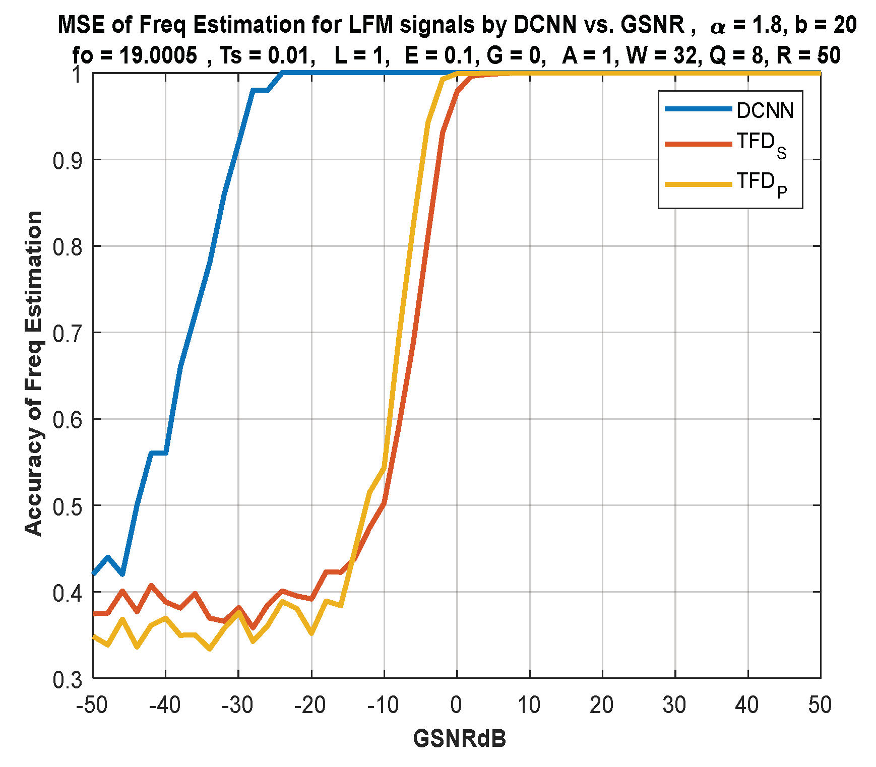
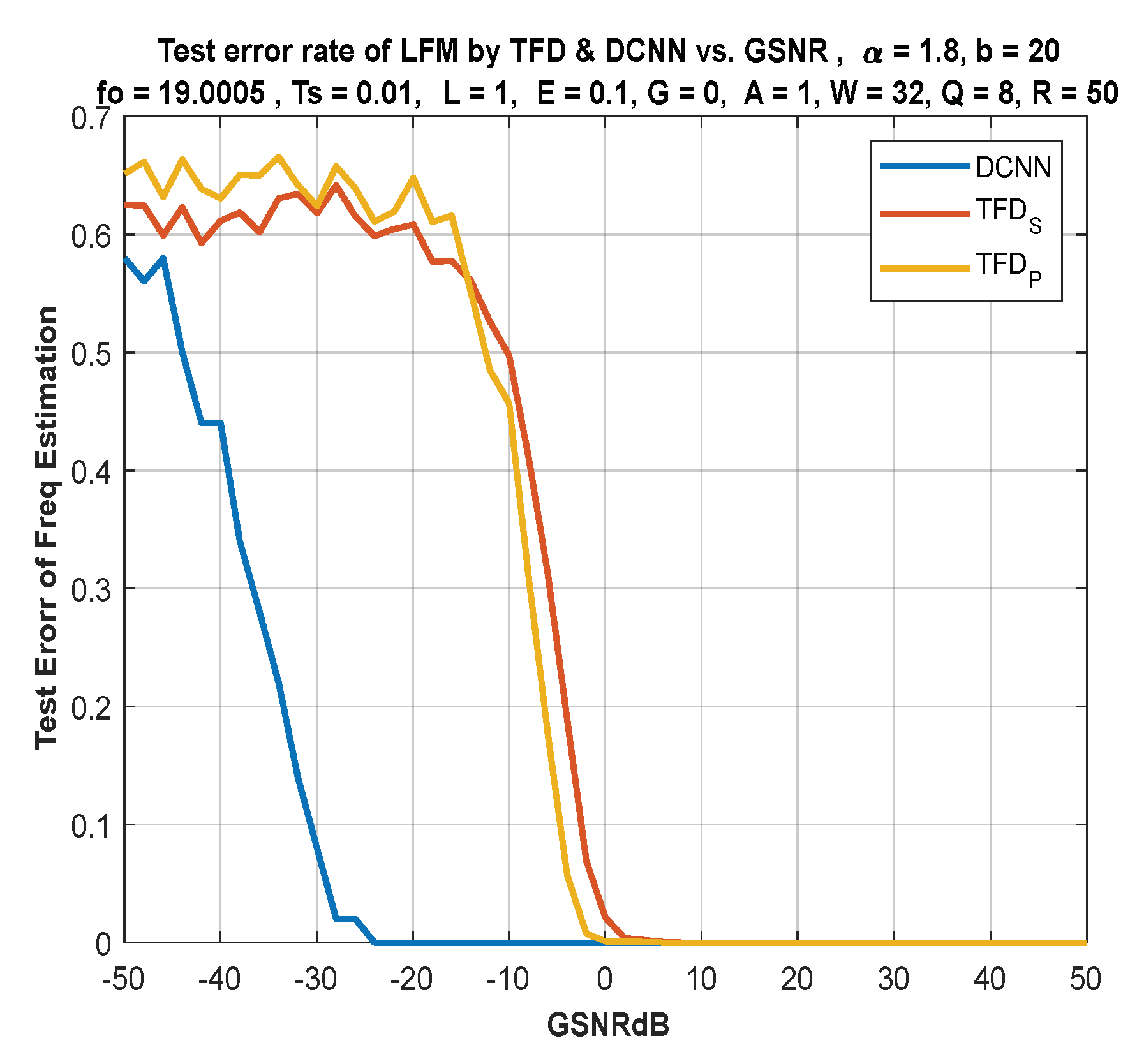
  • The performance of the DL approach is compared with the version of the still-active classical techniques based on Fourier analysis. It is shown that the classical time–frequency-based methods are ineffective under the damaging alpha-stable noise, especially under low signal-to-noise ratios, where a difference of 20 dB in performance has been noticed compared to the DL approach. This result is vital for underwater RADAR systems, where impulsive noise is dominant.
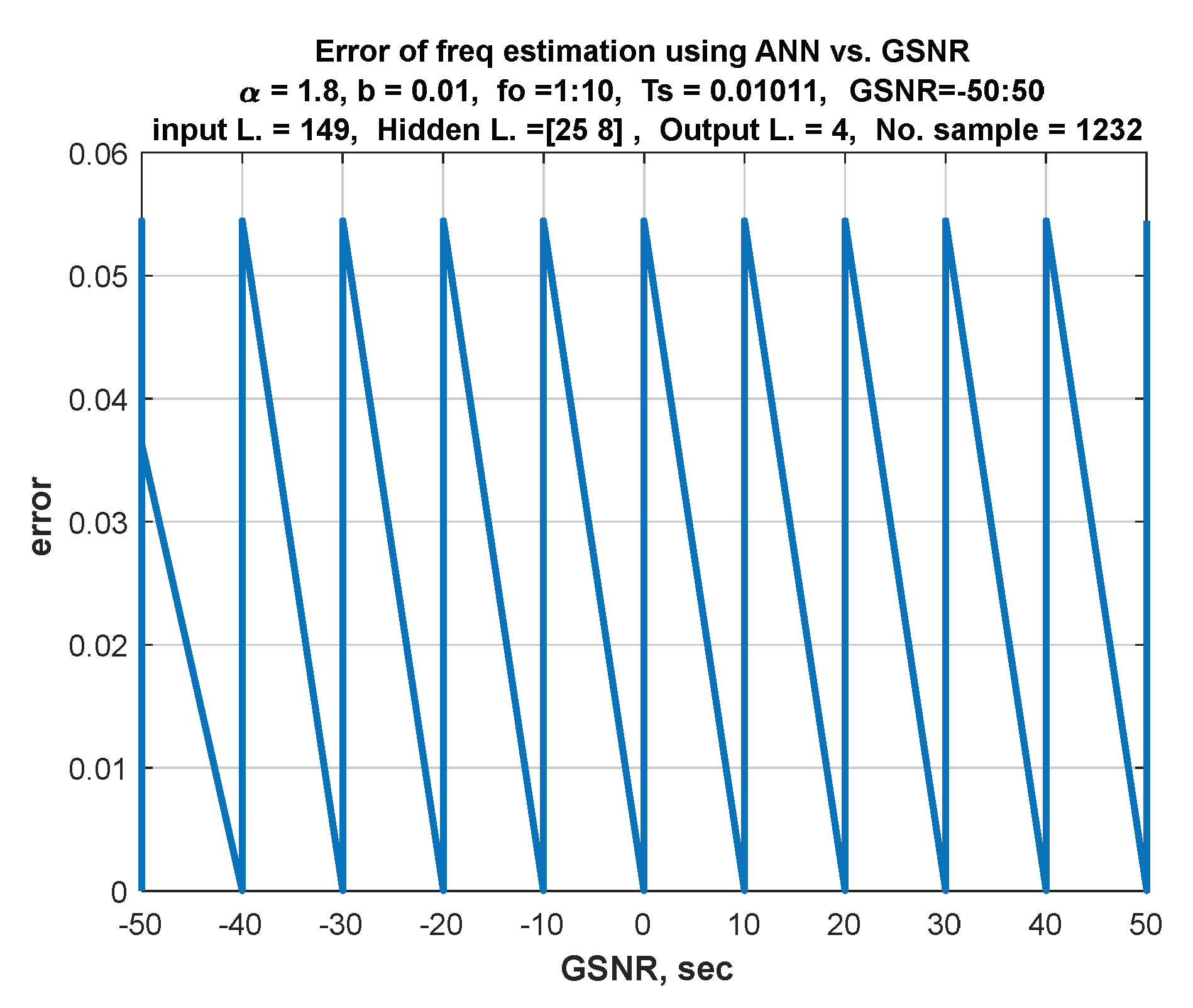
  • The DL approach is SNR-dependent, so an investigation of the system performance under various SNRs is presented. Based on our previous work [12], a change in SNR will have little effect on the performance of the DL-based approach.
  • The reduced complexity introduced by DL-based FE and avoiding complex valued arithmetic will make FE easier and cheaper for IoT communications, sensors, sensor networks, and SDR. This work presents discussions on such possibilities.

4. FM Signals and Noise

This section illustrates FM signals, AWGN, and SαS noise as follows:

4.1. Instantaneous Frequency and FM

A key feature of FM transmissions is the instantaneous frequency, which describes the fluctuations in frequency content across time. The IF of a signal is a time derivative of its instantaneous phase θ t [13,14]:
f t = 1 2 π d θ t d t
θ t = 2 π f o t + σ t 2 2 + ρ t 3 3
Note that the initial phase θ o has been omitted as it has no effect on the frequency estimation.
The signal model with LFM law used in this work is [15]:
s t = A   e j 2 π f o t + σ 2 t 2
where σ is the linear modulation index, f o is the initial frequency (in Hertz), and A is the amplitude. Using Equation (1), the LFM signal IF will be [16]:
f t = f o + σ t
The quadratic IF law has also been used to consider the quadratic frequency modulation (QFM) signal in this work:
s t = A   e j 2 π f o t + σ 2 t 2 + ρ 3 t 3
where ρ is the quadratic modulation index of the QFM signal, with the quadratic IF law:
f t = f o + σ t + ρ t 2

4.2. Additive White Gaussian Noise

AWGN has the following probability density function with zero mean and variance (power) υ 2 [13]:
F Z = 1 υ 2 π e Z 2 / 2 υ 2
where Z is a random variable and υ is the standard deviation of the noise.
The procedure for generating AWGN is as follows:
  • Calculating the power p x contained in the input signal x t , were
    p x = 1 L i = 0 L 1 | x i | 2 ,   L = x
  • Converting the supplied SNRdB ( SNR in d B ) to a linear scale and finding the noise power in terms of SNR and signal power p x , were
    SNR = 10 SNRdB / 10 ,   N 0 = p x / SNR
  • Using the following equations to determine the AWG noise:
    G = υ · Z .   if   x   is   real
    G = υ Z + i   M ,   if   x   is   complex
    where Z , M N 0 , υ 2 . For a real signal υ = N 0 , for a complex signal υ = N 0 / 2 .

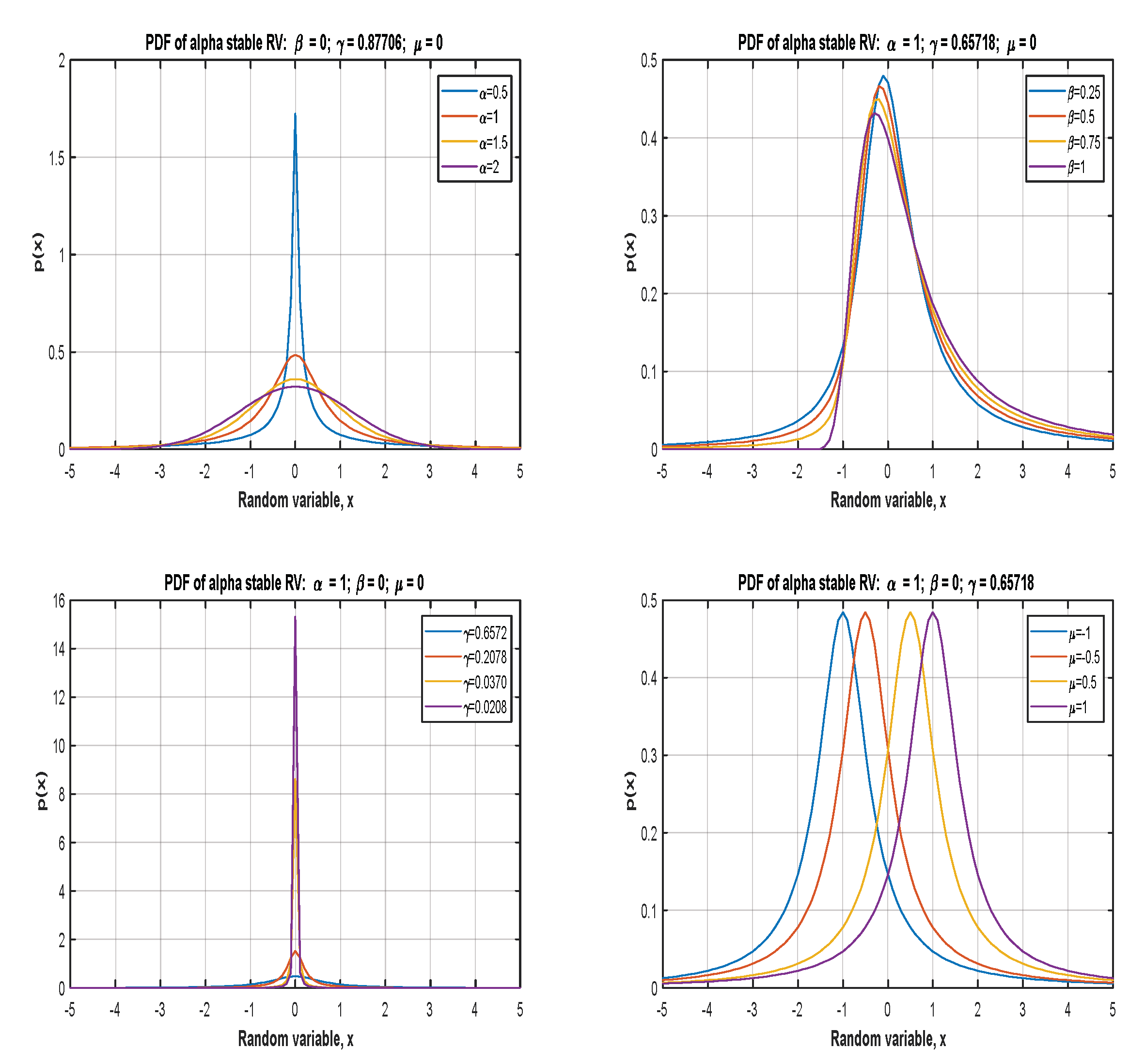
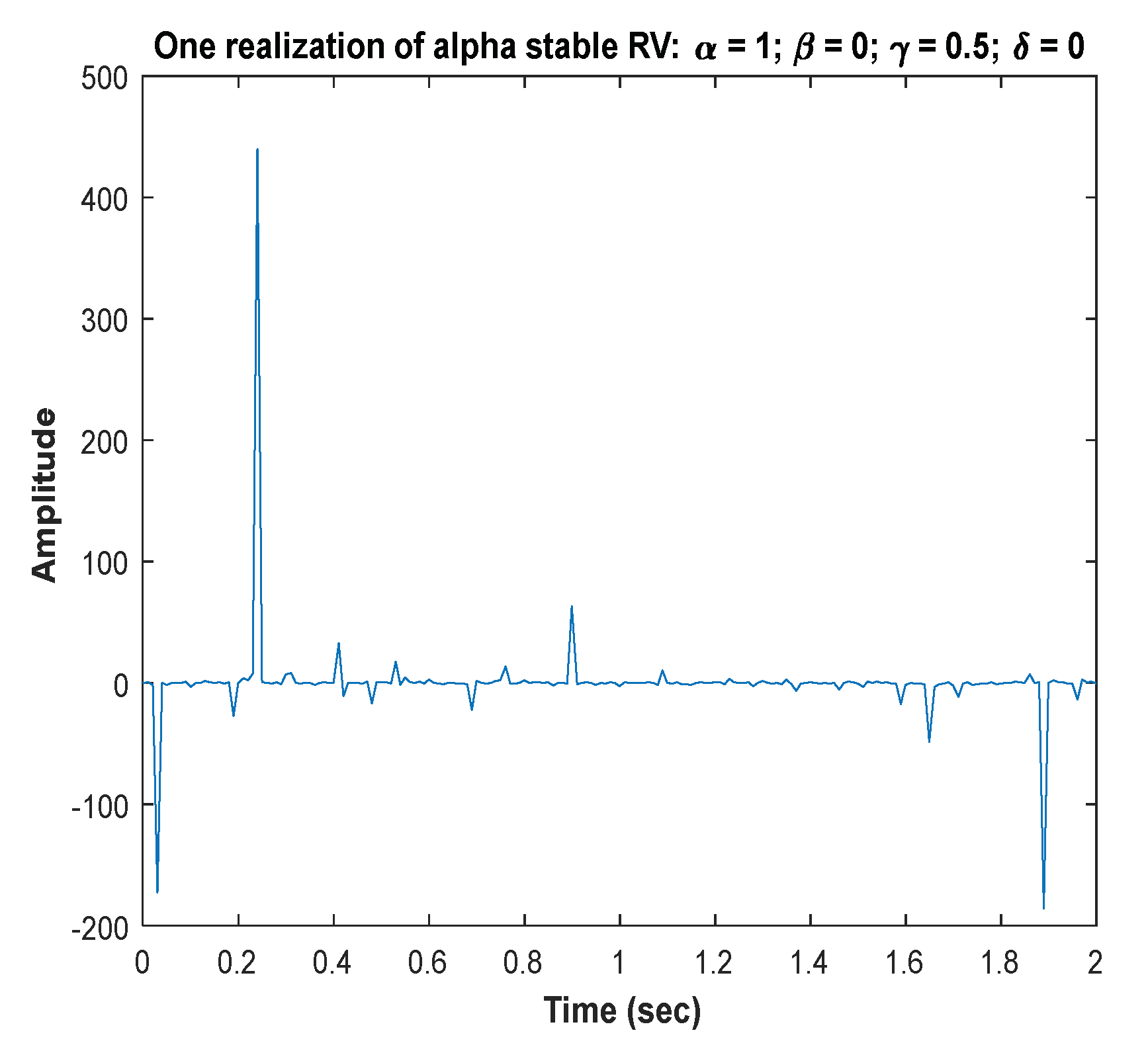
4.3. Symmetric α-Stable Noise

The α-stable distribution noise necessitates four parameters ( α , γ , β , and µ ), with the stable distribution characteristic function specified as [17,18]:
ψ ω = exp γ | ω | α   [ 1 + β sign ω W ω , α
W ω , α = tan α π 2   for   α 1 2 π log ω     for   α = 1
And sign( ω ) is the signum function.
The characteristic function for the SαS distribution when β = 0 is specified as follows:
ψ ω = exp γ | ω | α
where (0 < α ≤ 2) is also known as the tail index or characteristic exponent. When α < 2, the distribution is algebraic-tailed with a constant tail α, meaning infinite variance. The density of tails becomes heavier as it gets smaller. When α = 2, the SαS distribution is reduced to the Gaussian distribution. When α = 1 and β = 0, the SαS distribution is reduced to the Cauchy distribution. When α = 0.5 and β = 1, the SαS distribution is reduced to the Lévy distribution. The parameter γ > 0, usually called the dispersion, is a positive constant related to the distribution scale. The parameter γ plays a role that is analogous to that of the variance for a second-order process. The skewness parameter is β ∈ [−1,1]. The location parameter is µ     . The procedure of SαS simulation is explained in Appendix A.

5. The Proposed Method

This section explains the proposed method for estimating the frequency and slope. Deep learning and machine learning were used to predict the frequency and slope of noisy signals and then calculate the instantaneous frequency. Then it is compared with the time–frequency distribution as shown in the results. ANN includes feedforward neural network (FNN), the same multilayer perceptron (MLP). The input–output layer is called a single-layer network, and one hidden layer is called a shallow neural network. Two or more hidden layers are called DNN. The nodes in neighboring layers are fully connected. DNN with a complex structure is time-consuming for training [19]. The activation functions are chosen depending on the type of problem to be solved by the network. The most common activation functions are sigmoid or logistic and hyperbolic tangent or tanh [20]. SCG and adaptive moment estimation (Adam) are used as optimization algorithms in ANN. SCG uses second-order neural network information while requiring just O N memory use, where N is the number of weights in the network [21]. The procedures of Adam are explained in reference [22]. DL is a subset of machine learning. CNN is used in deep learning. A CNN type of deep ANN [23], consists of input, output, and hidden layers. CNN works with multiple hidden layers and 2D data, so the input data must be transformed into 2D matrices before it can detect frequency or slope. Each input image is passed through a series of convolution layers with filters (kernels), pooling, fully connected layers, and the Softmax function to train and test deep learning CNN models. CNN transforms manual feature extraction methods into automated processes [24,25]. Many metrics are used to evaluate ML and DL methods. The perfect models chosen using these metrics [26] include accuracy, precision, recall, F-measure, and receiver operating characteristic (ROC).
This paper demonstrates for the first time the estimation of FM parameters by deep learning, which is one of the main contributions, as most researchers use deep learning to classify the signals, where the proposed CNN model has less complexity than found models. We have not used pre-trained CNN models such as AlexNet, VGG, GoogLeNet, or ResNet, as they have more layers and complexity. The signal was used in the time domain because conversions to the frequency domain are complex and affect the efficiency of deep learning. We also propose the b ratio to combine the Gaussian noise and the symmetric α-stable noise to form a noisy signal.

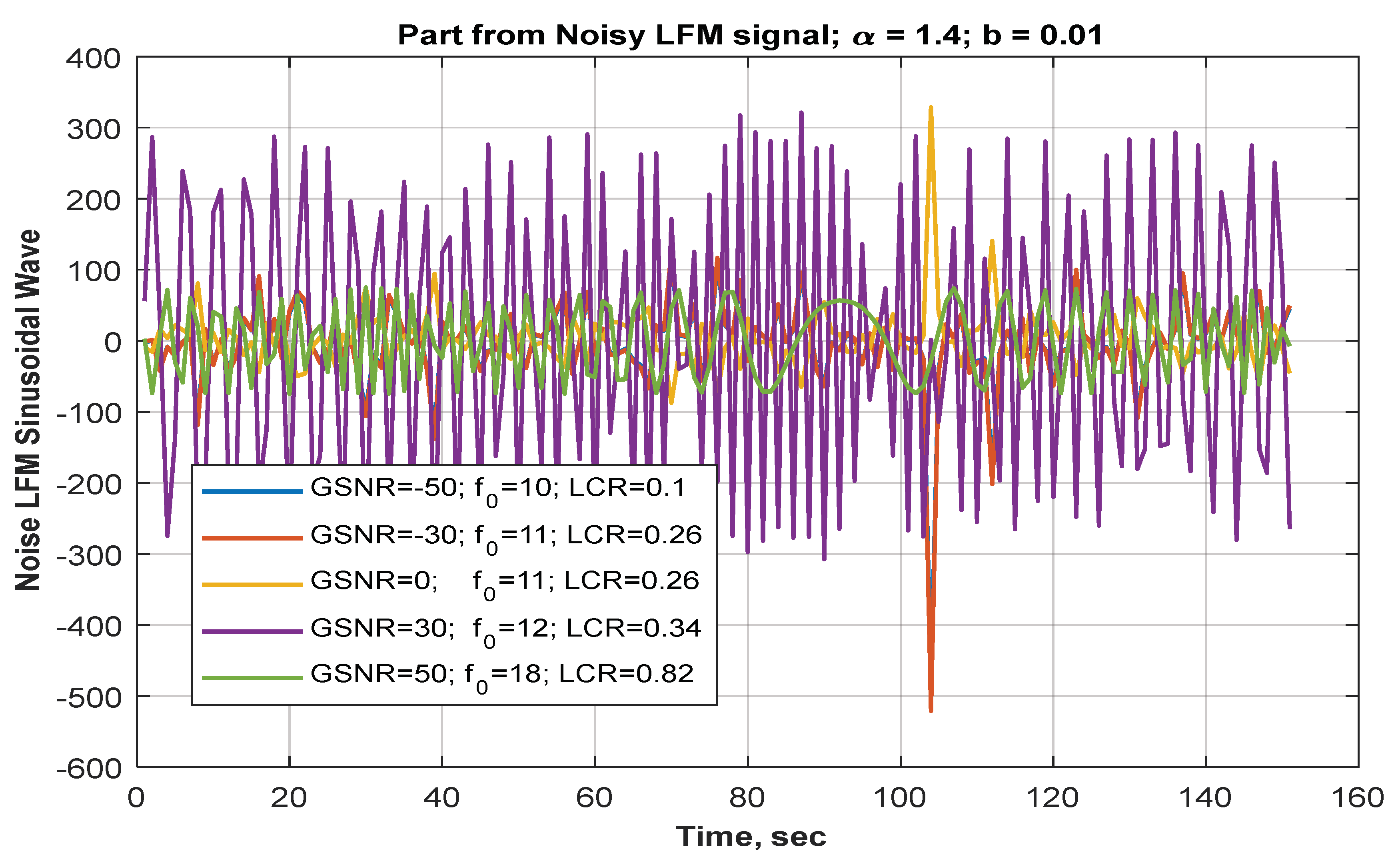
5.1. Hybrid Noise and Noisy Signal Generation

A nonstationary signal is one with a changing frequency content over time. This work is based on LFM signals influenced by noise (AWGN and S α SN). S α SN requires four parameters α ,   γ ,   β ,   µ . The most critical parameters are the tail index α and scale of the distribution ( γ > 0 ) , while the less essential parameters are β   and   µ . Gaussian noise is fixed power, and S α S noise is geometric power.
Geometric SNR (GSNR) is used to determine noise impulsiveness, characterized by zero-order statistics. Since all 2nd order moments are infinite, the standard SNR does not apply. The geometric power of S α S N is defined as follows:
p S = γ 2 .   C 2 α 1  
where C is the exponential of Euler’s constant, C = e E c   1.7811 , E c Is Euler’s constant E c = 0.5772156649 . When α = 2 , SαS noise is Gaussian with finite variance σ 2 = γ 2 .
GSNR   = p x / γ 2
GSNRdB   = 10 · log 10 GSNR
p x = A 2 / 2
In wireless networks, received signals are corrupted by the noise mixture of Gaussian ( G ) and S α S (Y ) noises. Total noise ( N T ) is represented in the equation as follows:
N T = G + Y
The overall GSNR is defined as follows,
G S N R = p x / p T
Let p T = p G + p S , where p T total noise power, and p G be the Gaussian power. We proposed b ratio, if p G = b · p S , then p T = 1 + b p S , p S = p T 1 + b , and
b = p G / p S
If b is less than one, then p G is less than p S , else p G is greater than p S . The scale parameter is:
γ = p S / C 2 α 1
Consider AWGN and SαSN affected by single-tone sinusoidal and FM signals as follows:
x t = A cos θ t + 0 + N T
where A is the signal amplitude, and 0 is an initial phase. The single tone and LFM signals are generated, where the amplitude of signals is A = 1 , signal power is p x = A 2 2 , initial phase φ o = 0 . To find the instantaneous phase as shown in Equation (2), the frequency and LCR are computed as follows:
  • The frequency ( f o ) range:
    • Initial frequency is f 1 = 10
    • Final frequency is f 2 = 19
    • The number of frequencies is n f = 10
    • The differential frequency step is d f = f 2 f 1 / n f
    • The range of frequency is f o =   f 1     increasing   by   d f     f 2
  • The LFM slope ( σ ) range:
    • Initial slope is e 1 = 0.1
    • Final slope is e 2 = 0.9
    • The number of slopes is n e = 10
    • The differential frequency step is d e = e 2 e 1 / n e
    • The range of slope is σ = e 1     increasing   by   d e     e 2
  • The time vector ( t ) range:
    • Initial time is t 1 = 0
    • Final time is t 2 = 640
    • Sampling period is T s = 0.1
    • The range of time in seconds is t = t 1     increasing   by   T s   t 2 T s
The following procedure shows a summary of hybrid noise N T Generation:
  • GSNR range is chosen as 50   50 dB .
  • To generate S α S as shown in Equations (27b), (33) and (35) with four parameters chosen as follows: α = 1.8 , β = 0 ,   µ = 0 , while the choice of γ is (scale parameter) relies on the ratio b = 20 as shown in Equation (19).
Total power is p T = p x / GSNR as shown in Equation (17).
S α S geometric power is p S = p T / 1 + b and p G = b × p S as explained in the line above Equation (18).
The AWGN power is p n d B = 10 · log 10 p G .
  • AWGN ( G ) is generated as shown in Equation (10).
  • Total noise ( N T ) is a hybrid: AWGN with S α SN , as shown in Equation (16).

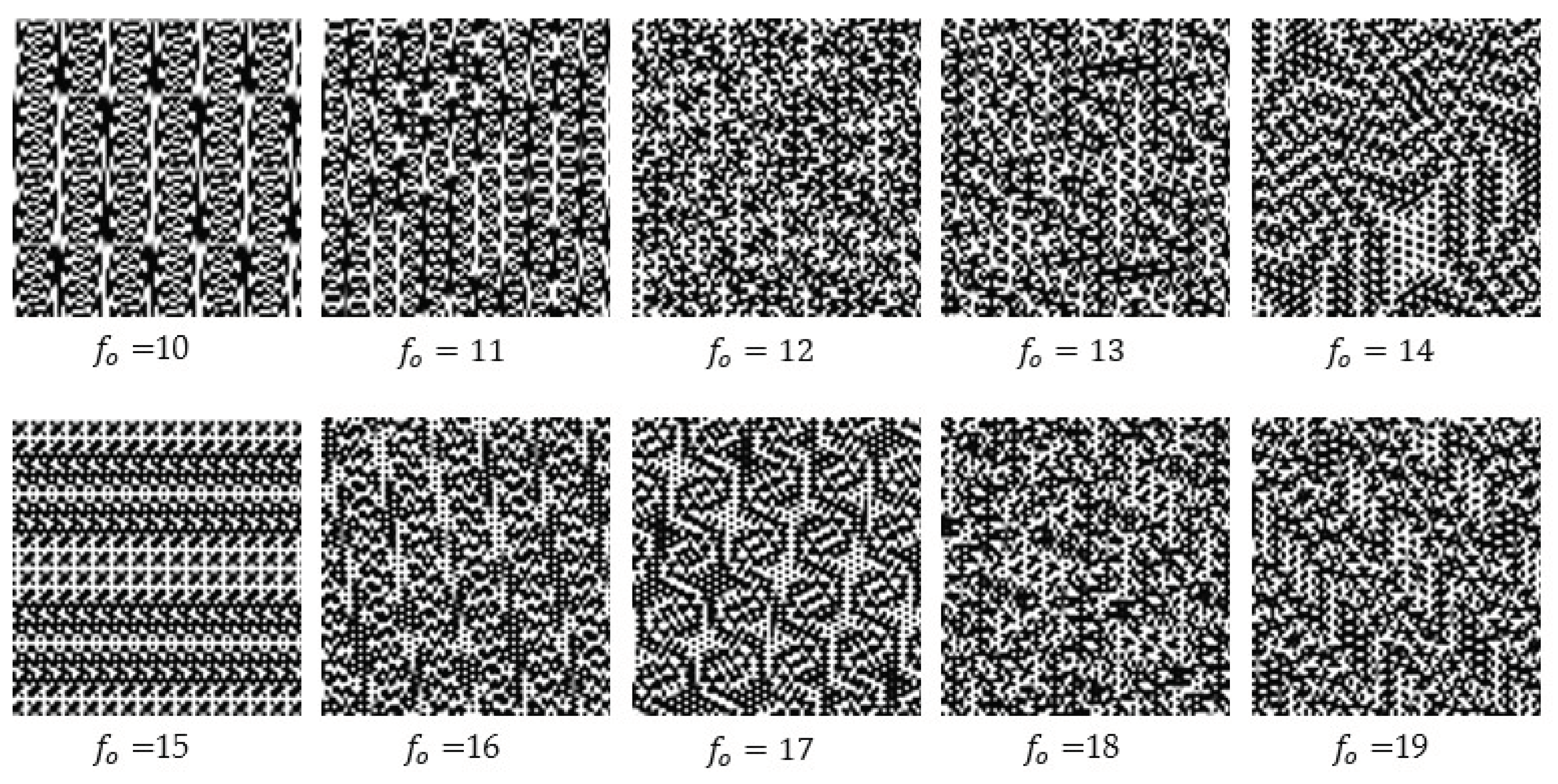
5.2. Converting 1D Signal into 2D Signal and Dataset Creation

After the noisy LFM signals are generated in the time domain with 1-dimensional (1D) signals and length 6400, it is converted into 2-dimensional (2D) with size [80 80] and in the time domain because CNN deals with 2D signals. An example illustrating how to convert a 1D signal in the time domain into a 2D signal, let input 1D-signal with length 9 is as follows:
I n p u t s i g I D = 1   2   3   4   5   6   7   8   9
It converts into 2D signals with a length of 3 × 3 as follows:
O u t p u t s i g 2 D = 1 2 3 4 5 6 7 8 9
Data are converted to the graphics format of an image. The images are represented as two-dimensional arrays (matrices) and stored in one of the graphics file formats, such as tagged image file format (TIFF).
After reshaping the input signal into 2D, it saves it as a TIFF type in a folder. The proposed CNN is then trained using 2D signals or images as input. The 1D signals are converted into 2D signals as explained in Algorithm 1.
Algorithm 1: Converting 1D Signals into 2D Signals
Input:   The   noisy   signals   1 D   in   the   time   domain   ( N S i g n a l ).
Output:   The   noisy   signals   with   2 D   ( O u t s i g 2 D ) .
Begin:
  1.For h 1   t o   N S    //   N S = 12120
  2. initial counter k 1 , where k 1     6400 .
  3. tack the values from s i g 1 D and place in s i g 2 D column by column and row by row as follows:
  4. s i g 1 D = N s i g n a l h
   5. For i 1   t o   R   // R = 80
    6. For j 1   t o   C   // C = 80
      7. s i g 2 D i , j s i g 1 D k
      8. k k + 1
    9. End for j
  10. End for   i
  11. Save   the   s i g 2 D   with   TIFF   type   in   folder ,   where   O u t s i g 2 D = s i g 2 D   . TIFF
  12. End for   h
  13. Return O u t s i g 2 D in folders.   // name folder is label.
End algorithm

The Dataset Generates

The dataset was created after converting signals into 2D, containing ten folders and the name folder is the label, each representing one class. Each class has an IF and an LCR. The number of samples in each class equals the number of GSNR samples 101 multiplied by the number of realizations 12 , which equals 1212 . The total number of samples in the dataset equals the number of samples in each class multiplied by the number of classes 12120 . The target or true label of samples denotes 0   9 , which represents the number of frequencies and slopes. The dataset is randomly divided into 80% for the training set, 10% for the validation set, and 10% for the testing set, where Algorithm 2 illustrates the dataset divided, where noisy LFM signals dataset denoted D a t a _ X and labels denoted by D a t a L .
Algorithm 2: The Dataset is Divided into Training, Validation, and Testing Sets
Input:   Noisy   LFM   signals   dataset   D a t a _ X   and   labels   D a t a L , where each label is presented as frequency and slope.
Output: Noisy LFM Signals divided into a training   set   X T r ,   L T r ,   validation   set   X V a ,   L V a ,   and   testing   set   X T e ,   L T e .
Begin:
  1. Select a random index as the following:
    Rind = Random N   , where N = D a t a _ X
  2. Sorted dataset according to R i n d as follows:
         X = D a t a _ X : , Rind ,             L = D a t a _ L : , Rind      
  3. Select the length of training, validation, and testing percent:
    T r = N × 0.8  
    V a = N × 0.1  
    T e = N × 0.1  
  4. Divided dataset into a training set ( X T r ) , and labels ( L T r ) as follows:
    X T r = X : ,   1 : T r
    L T r = L : ,   1 : T r
  5. Divided dataset into validation set ( X V a ) , and labels ( L V a )   as follows:
    X V a = X : , T r + 1 : T r + V a      
    L V a = L : , T r + 1 : T r + V a      
  6. Divided dataset into the testing set ( X T e ) , and labels ( L T e ) as follows:
    X T e = X : , T r + V a + 1 : T r + V a + T e  
    L T e = L : , T r + V a + 1 : T r + V a + T e  
  7. End of algorithm

5.3. Estimation of IF and LCR by DNN

A deep neural network (DNN) is used for IF and LCR estimates. It contains the network’s components and represents the network’s structure. It also needs two phases, forward and backward, for training and predicting the output. Each of them is explained as follows:
DNN structure includes an input layer, two hidden layers, and an output layer. The input layer contains twenty nodes. The number of nodes in the first and second hidden layers is 25 and 8, respectively. The output layer has four nodes (the number of classes).
DNN forward stage, in which the training set is used, finds the sum of the product of input nodes with corresponding weights, then adds bias. The initial weights and biases are generated at random. Then an activation function is applied, where the first and second hidden layers use ReLU for activation. The output layer’s activation function is sigmoid. The most important term in the loss expression is an error. There are numerous cost functions. In this work, cross-entropy was used to compute the error for each node in the output layer and the loss value. When the error (the difference between the desired and expected output) is greater than a certain threshold, the neural network stops training, or the neural network stops its access to the last epoch.
DNN backward stage applies an optimization algorithm to update the parameters (weights and biases) and compute the error ratio for each layer in the backward path based on gradient descent, as shown in the optimization algorithm. The optimization algorithm governs how the network’s parameters are adjusted. The scale conjugate gradient (SCG) optimization algorithm is used in this work to update weights and biases. The maximum number of epochs for stope training is 1000, and the learning rate is 0.0001. The update is given by:
New _ parameters = Old _ parameters + R SCG × learning _ rate
where New _ parameters are new weights and biases, Old _ parameters are older weights and biases, and R SCG = α k p k , α k is the k th (adaptive) step-size and p k is the search direction as explained in reference [12,21], noting that SCG updates the weights and biases relying on the derivative of the loss (entropy). The derivative of the entropy is applied in the backward stage for DNN as gradient descent, while the loss is applied in the forward stage for DNN to measure the performance of a network.
Evaluation of the training set for each epoch is performed using a validation set. The validation loss is similar to the training loss and is calculated as the sum of the errors for each sample in the validation set. Forward and backward steps are performed until reaching the last epoch (end of training), where the trained DNN model is returned.
The final step is to test the DNN model with a testing set, where a testing data set is applied to the trained DNN model to predict the label. Then the DNN model’s evaluation is performed using some metrics such as accuracy.
After the label’s prediction, it is possible to estimate the frequency and slope to which it belongs. Then the amount of error and the accuracy between the predicted parameters and the true parameters are calculated as follows:
  • True frequency ( T f ) is the target frequency of a signal
  • Estimate frequency ( P f ) is the predicted frequency of the DNN network
  • The relative absolute error of the frequency E f = T f P f / T f
  • True slope ( T S ) is the target slope of a signal
  • Estimate slope ( P S ) is the predicted slope of the DNN network
  • The relative absolute error of the slope is E s = T s P s / T s
  • Estimate IF is I F = P f + P s   t
Figure 1, Figure 2, Figure 3, Figure 4, Figure 5 and Figure 6 explain the several essential cases to show the effect of feature extraction and deep neural network design on the error rate, frequency, and slope estimation accuracy. Figure 7 shows GSNR vs. RMSE of FE for noisy LFM by DNN. Figure 8 shows the ROC of FE for noisy LFM by DNN. Figure 9 shows a confusion matrix for noisy LFM by DNN.

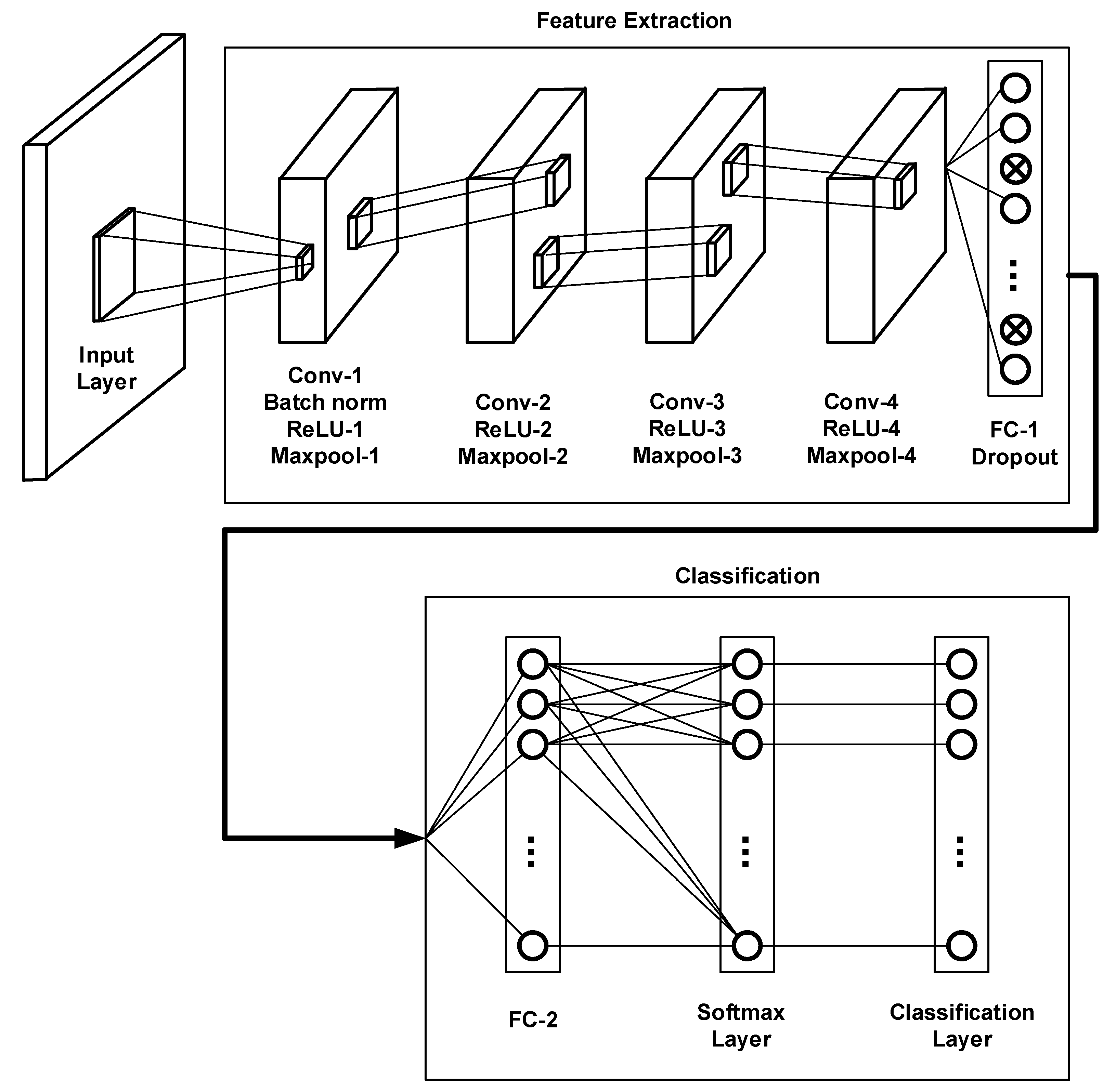
5.4. Estimation of IF and LCR by CNN

The CNN model’s input layer includes a training set with 2D. The hidden layer (feature extraction stage) includes convolution, batch normalization, ReLU, max pooling, fully connected, and dropout. The output layer (classification stage) consists of a fully connected, softmax classification layer. The number of nodes in the input layer is 80 × 80 . The number of nodes in the hidden layer is based on the parameters for each layer. The number of nodes in the output layer equals ten; it represents the number of labels. The convolution layer includes 30 filters, where the filter size is 3 × 3 , and the stride equals 1 × 1 . Other convolution layers have different numbers of filters: 60 ,   90 ,   and   128 ; max pooling with size 2 × 2 , stride 2 × 2 , zero padding; fully connected layer with 100 output nodes in feather extraction stage. The dropout layer ratio is 50 % . A fully connected layer has ten output nodes in the classification stage. The classification layer uses cross-entropy. These layers are explained in Appendix B as shown in Table A1. Figure 10 shows the proposed CNN model layers. Algorithm 3 illustrates the CNN model procedure. CNN contains the network’s components and represents the network’s layers and options. It also needs two phases, forward and backward, for training and predicting the output. Each of them is explained as follows:
Forward Stage of CNN Model:
  • Batch normalization is applied on input signals; it speeds up training by halving the epochs (or faster).
  • Feature map is found by computing the sum of product for input node with weights (filters), then summation with bias is performed, where bias is used in the forward stage.
  • An activation function is applied to the sum of the product, where the activation function is ReLU.
  • Max pooling is applied; it is used to decrease the size of the feature maps.
  • The convolution layer is applied three times with the number of filters (60, 90, and 128), and each of them is followed by a ReLU layer and max pooling layer.
  • A fully connected network is applied: it is a feedforward neural network where all of the inputs from the previous layer are linked to each node in the next layer.
  • Dropout is applied: it is a method of stochastic regularization. It aids in the prevention of overfitting, and the accuracy and loss will gradually improve.
  • The classification stage includes three layers that are fully connected, followed by softmax, then a classification operation. The fully connected layer has ten output nodes: a feedforward neural network. The softmax is utilized as the activation function in the output layer for multi-class classification tasks. The loss function is finding the error for a single sample in data training that relies on actual and predicted labels. The loss function is cross entropy loss used to measure how well a classification model in deep learning performs. The loss (or error) is calculated as a number between zero and one, where the zero value referred the perfect model. The cost function is the summation of the loss function for all data training. The objective function is referred to as a cost function (cross-entropy).
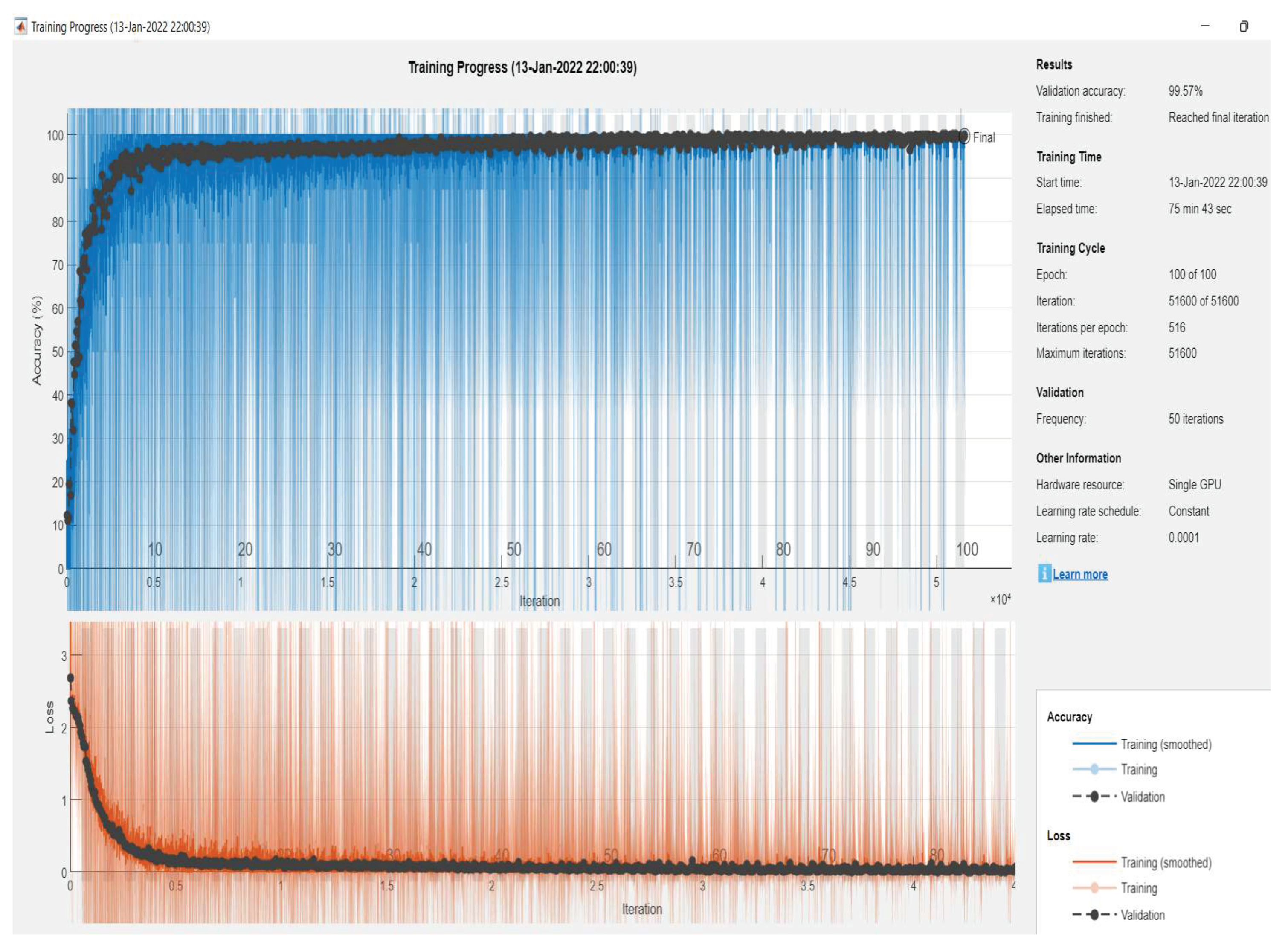
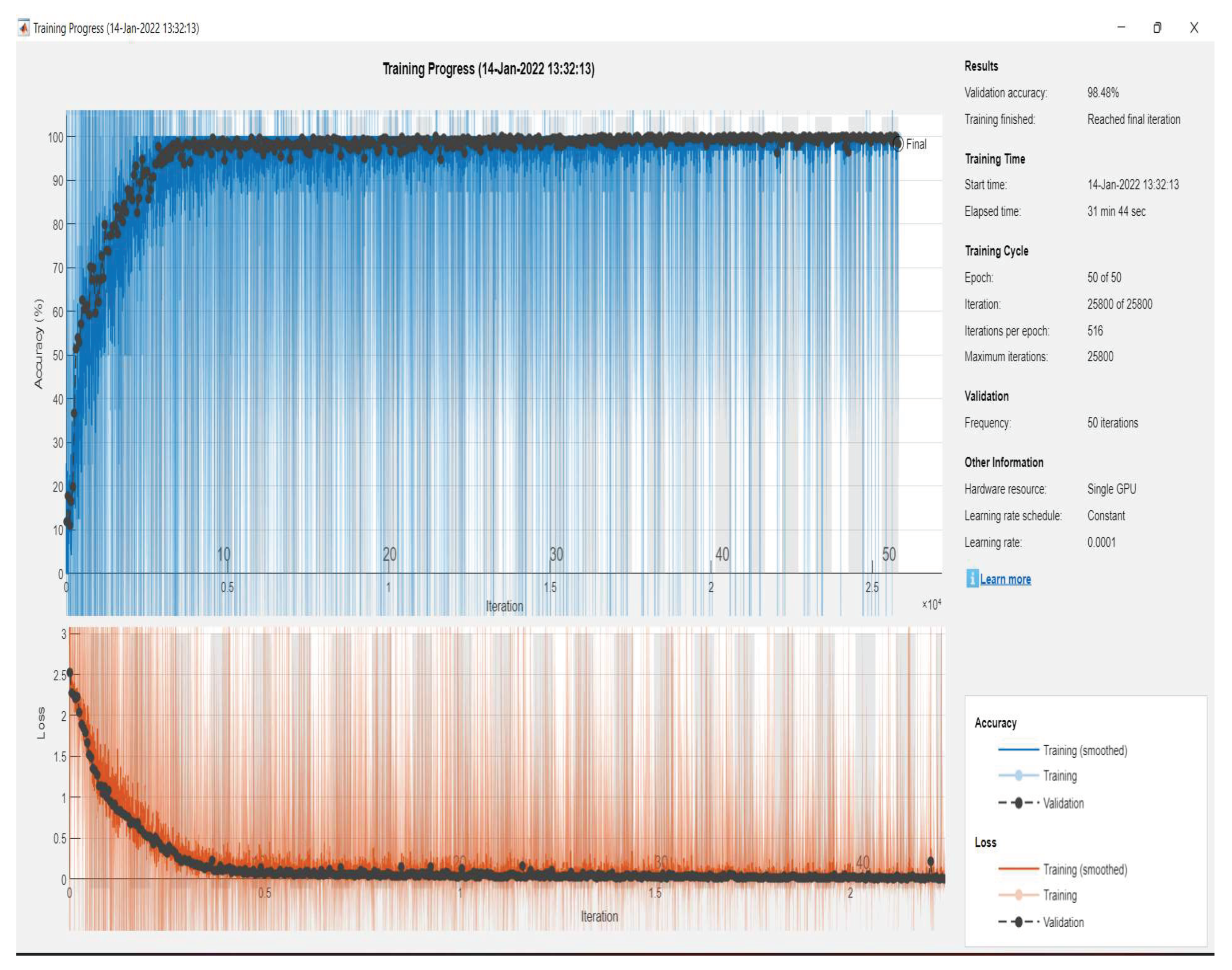
  • The parameters of the CNN model are a learning rate of 0.0001, max epochs are 5, and mini-batch size is 8. At the same time, Adam uses an initial learning rate is 0.001, Epsilon is 0.00000001, squared gradient decay factor is 0.999, and Gradient decay factor is 0.9. Hyperparameters in convolution are: the number of filters (30, 60, 90, and 128), the filter size is 3 × 3 , and padding and stride are equal to one. In batch normalization, the parameters are ε , Β , and λ , max pooling uses the size 2 × 2 , and the stride is 2 × 2 . In the dropout layer, the probability of dropout is 50%, and in the fully connected layer, the number of classes is 10.
Backward Stage of CNN Model:
  • In this stage, an optimization algorithm is needed to update the parameters, and each layer’s error should be calculated. The optimization algorithm controls how the parameters of the neural network are adjusted. In this work, Adam is used as the optimization algorithm
  • The weights and biases update is given by:
    New _ parameters = Old _ parameters + R Adam × learning _ rate
  • where New _ parameters are new weights and biases, Old _ parameters are old weights and biases, and R Adam = m t ~ / v t ~ + ϵ as explained in reference [22], Adam is updating the weights and biases relying on the derivative of the loss function (entropy). The derivative of the loss function is applied in the backward stage for CNN, while the loss function is applied in the forward stage for CNN. It measures the performance of the network. The training set is evaluated for each epoch using the validation set. The validation loss is similar to the training loss and is calculated as the sum of the errors for each sample in the validation set. Forward and backward stages are performed until reaching the last epoch (end of training).
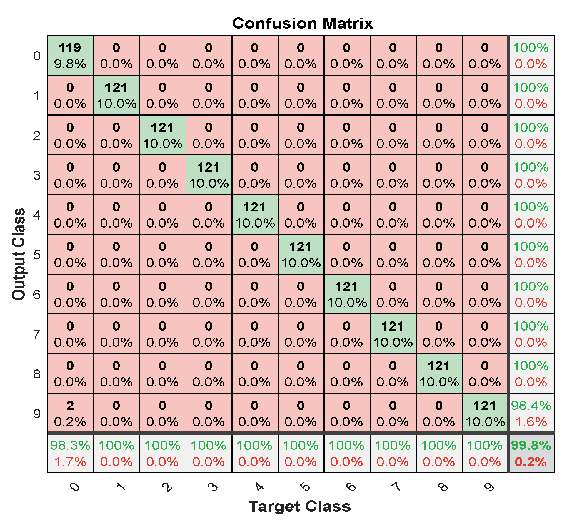
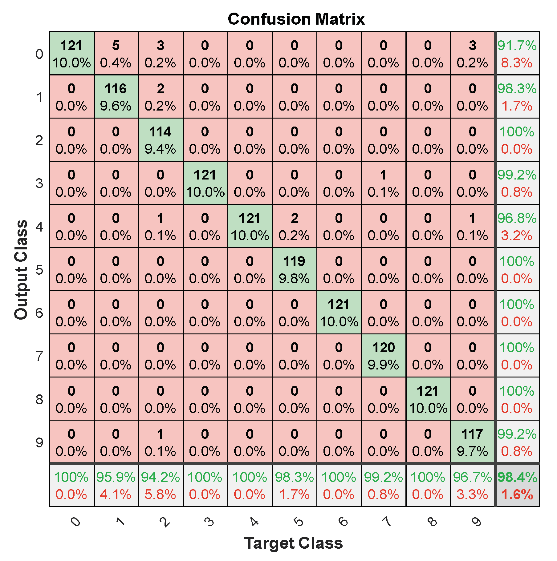
  • The final step is to evaluate the CNN model by applying a testing set to the trained CNN model to predict the label (class) for the test data. The CNN model is evaluated using relevant metrics such as accuracy.
  • After the class number (label) prediction, it is possible to estimate the frequency and slope to which it belongs. Then it is possible to calculate the amount of error and the accuracy of the predicted parameters versus the true parameters as follows:
    • True frequency ( T f ) is the target frequency of a signal
    • Estimate frequency ( P f ) is the predicted frequency of the CNN network
    • The relative absolute error of the frequency E f = T f P f / T f
    • True slope ( T S ) is the target slope of a signal
    • Estimate slope ( P S ) is the predicted slope of the CNN network
    • The relative absolute error of the slope is E s = T s P s / T s
    • Estimate IF is I F = P f + P s   t
Algorithm 3: CNN Model Procedure
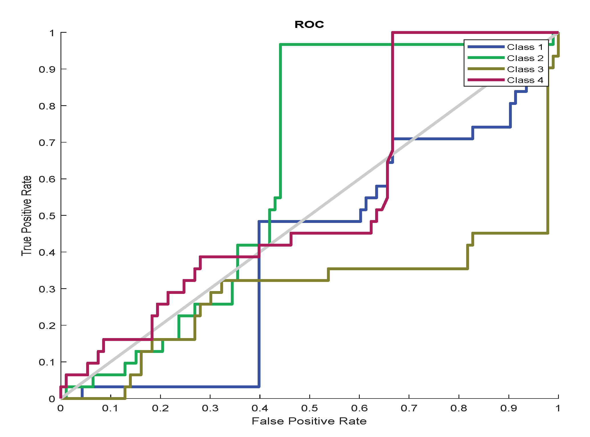
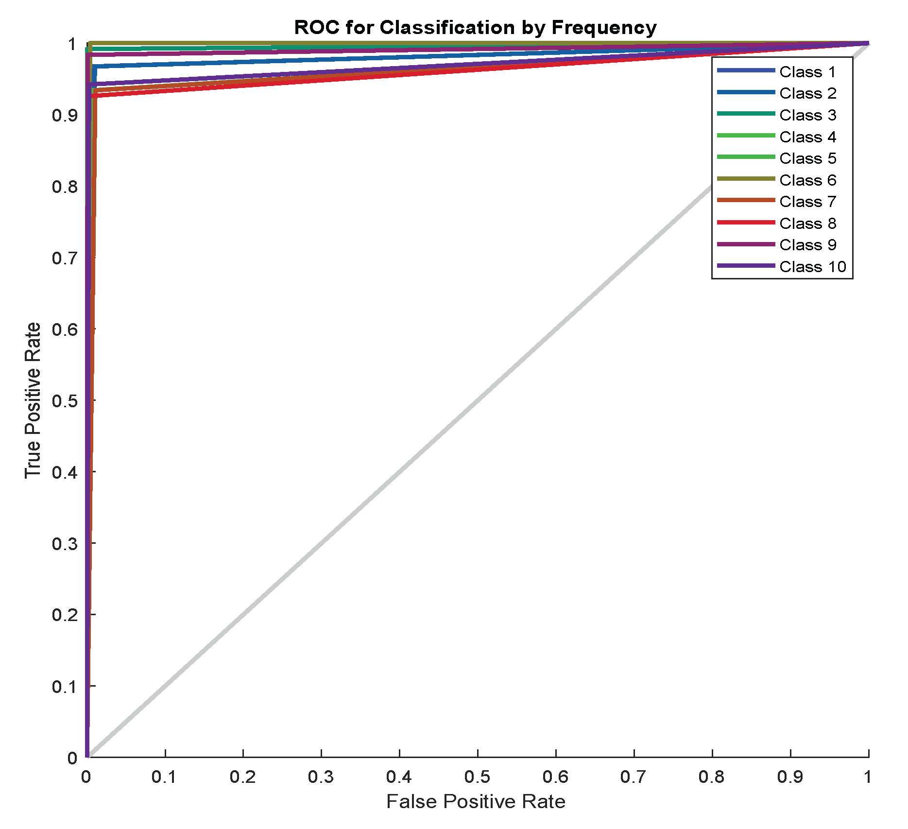
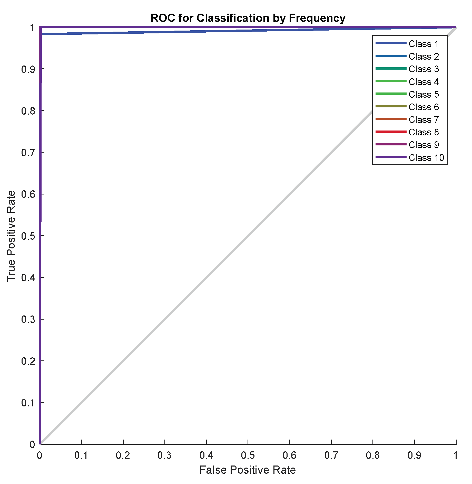
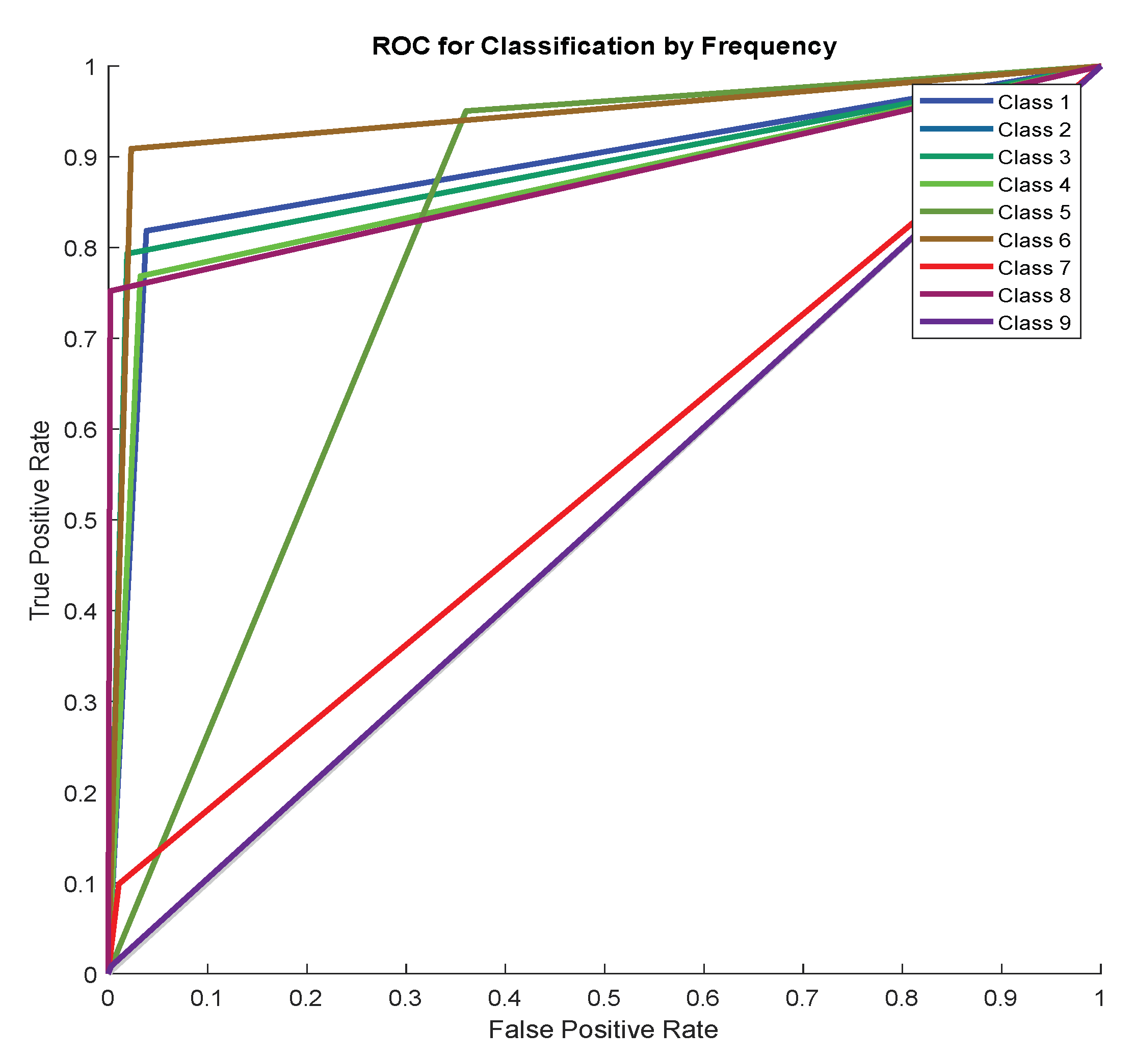
Input: Training   set   X T r ,   L T r ,   validation   set   X V a ,   L V a ,   and   testing   set   X T e ,   L T e , where each label is represented by the target   frequency   ( T f )   and   target   slope   ( T S ) .
Output: Frequency and slope estimation.
Begin:
Step 1: A training stage
  1. The input layer is the training set X T r ,   L T r with length N , and validation set X V a ,   L V a .
  2. Divided training set into min-batches, where mini-batch size M B equals 8. Iteration is one-time processing for forward and backward for a batch of samples. Iterations per epoch = number of training samples ÷ mini-batch size. Iterations = iterations per epoch × number of epochs.
  3. Find the batches, where b a t c h e s = N M B S .
  4. Find batch list, where b l i s t =   1   M B   N M B + 1
  5. For epoch =1 No of epoch
  6. For iteration =1 batches
  7. Select data by b = b l i s t iteration
  8. For k = b b + M B 1
  9. The convolutional layer applies convolutional operation between input signals and filters, where the number of filters equals 30.
  10. A batch normalization layer is applied as a result of step 2.
  11. ReLU is used as an activation function.
  12. Max pooling layer is applied to reduce the features map.
  13. The convolution layer is applied with several filters 60 to find feature maps, and then ReLU and max pooling layer are used.
  14. The convolution layer is applied with several filters 90 to find feature maps, and then ReLU and max pooling layer are used.
  15. The convolution layer is applied with the number of filters 128 to find feature maps and then used, ReLU and max pooling layer.
  16. A fully connected layer and dropout layer are applied to avoid overfitting.
  17. A fully connected layer is used with an equal output number of classes.
  18. Softmax is applied to find the output of the network that presents the predicate label ( L T r ^ ) , where each label is predicate frequency and slope.
  19. In the classification layer, calculate the performance of the network by entropy as follows:
E T r j = i = 1 n L T r i log L T r ^ i

   where n is the number of classes, L T r ^ i is predicate labels, L T r i is actual labels in one-hot encoding, j 1 , ,   N , N is the number of samples training.
  20. In the backward stage, calculate the error by the derivative of the loss function and compute the change of the weights ( Δ w ) as follows:
E = L T r L T r ^
M L k = L T r = L T r ^
Δ w = m ^ t v ^ t + ϵ    

  21. End of k loop
  22. Cross entropy is computing the cost function of the network. The sum of loss for each batch in the training set calculates the cost function of the training loss function:
L o s s T r = 1 N j = 1 N E T r j

   Then compute the accuracy of the training data set:
A c c T r = M L size   of   minibatch

  23. The weights ( w t ) are updated as follows:
w t = w t 1 η .     Δ w

  24. Evaluate the network during training by using validation data for each iteration, where applied same network layers on validation data and new weights are used to predict the label of validation data, and the cost of loss for validation is similar to the cost of loss for training as follows.
   Moreover, find loss as follows:
L o s s V a = 1 N v i = 1 N v j = 1 n L V a i j log L V a ^ i j
   where n is the number of classes, L V a ^ i j is predicate labels, L V a i j is actual labels in one-hot encoding, j 1 , ,   N v , N v is number of validation samples. The accuracy of validation is:
A c c V a = j = 1 N v L V a j = L V a ^ j N v

  25. End of iteration
  26. End of epoch
  27. CNN model trained ( C N N T r a i n ) is returned.
Step 3: Testing stage
   1. The testing set X T e ,   L T e It used the CNN model trained, which has the same layers but uses optimal weights.
   2. The CNN trained is applied on the testing set to predict the label, where each label is predicate frequency and slope.
    ● Estimate frequency ( P f ) is predicted frequency and estimated slope ( P S ) is the predicted slope from the predicated label ( P l a b e l ) of CNN network as follows:
P l a b e l = C N N T r a i n X T e

    ● Compute the error of frequency and slope as follows:
    ● The relative absolute error of the frequency E f = T f P f / T f
    ● The relative absolute error of the slope is E s = T s P s / T s
    ● Estimate IF is I F = P f + P s   t
   3. Evaluation of the CNN model trained using metrics is accuracy, precision, recall, F-Measure, and ROC.
End of algorithm

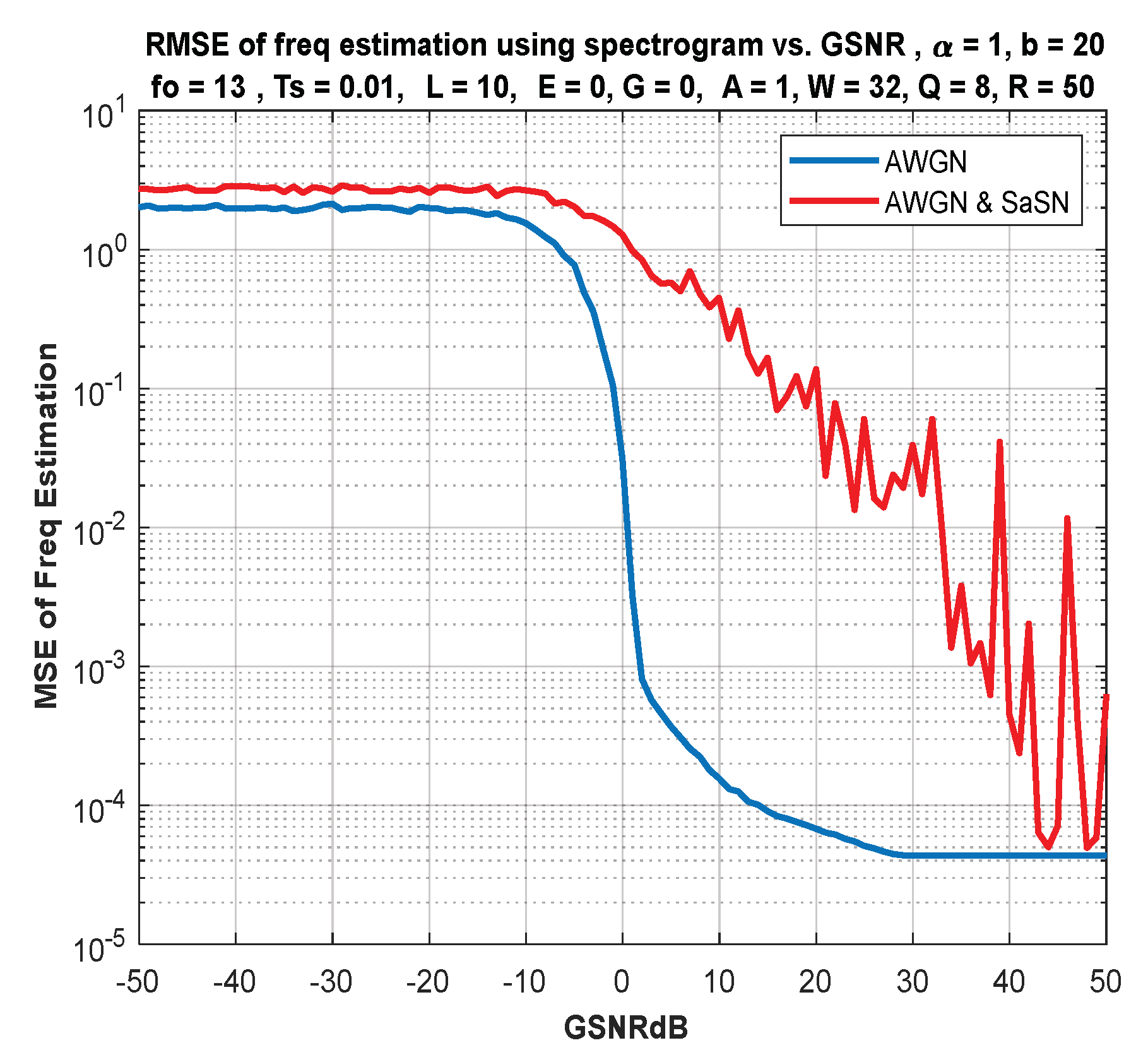
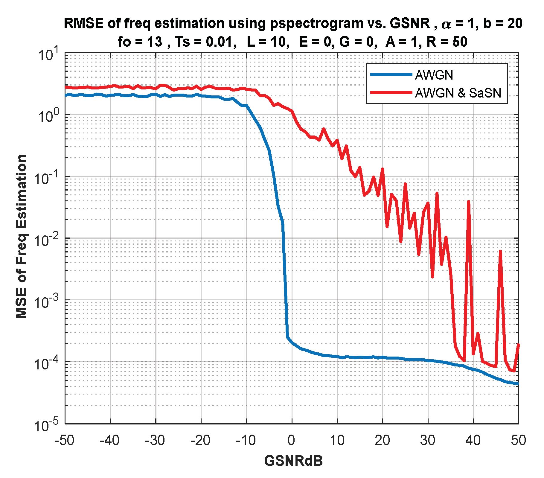
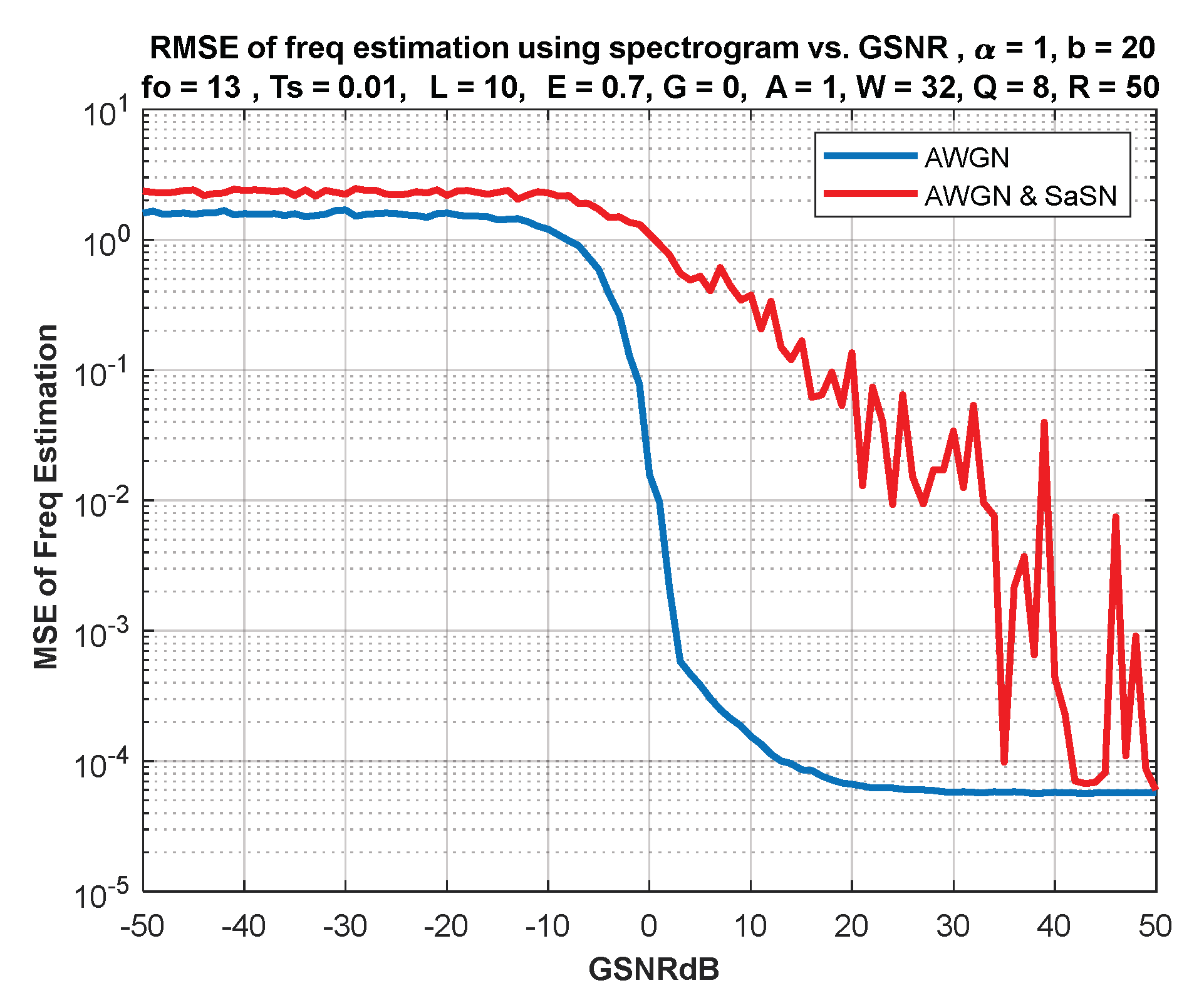
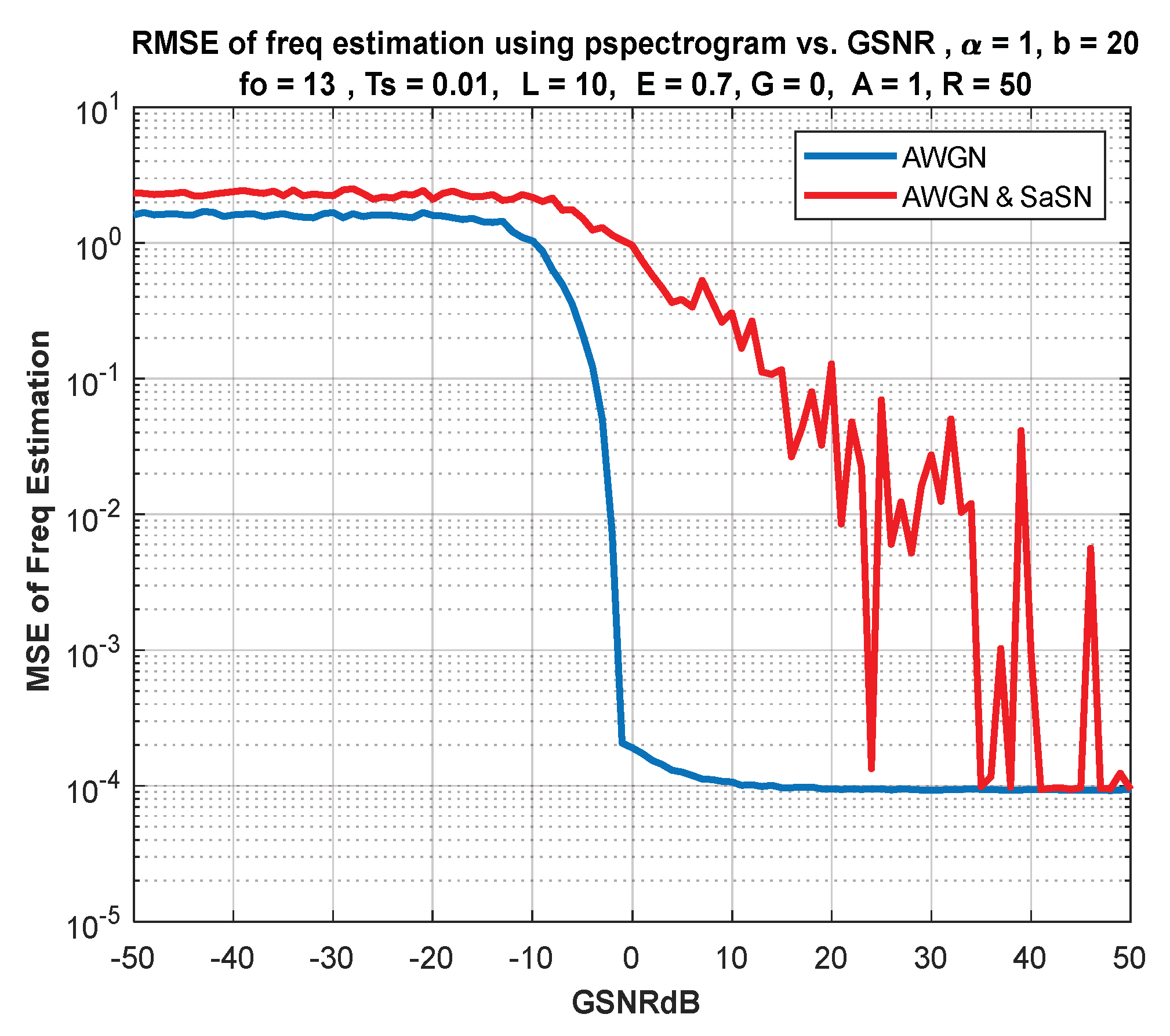
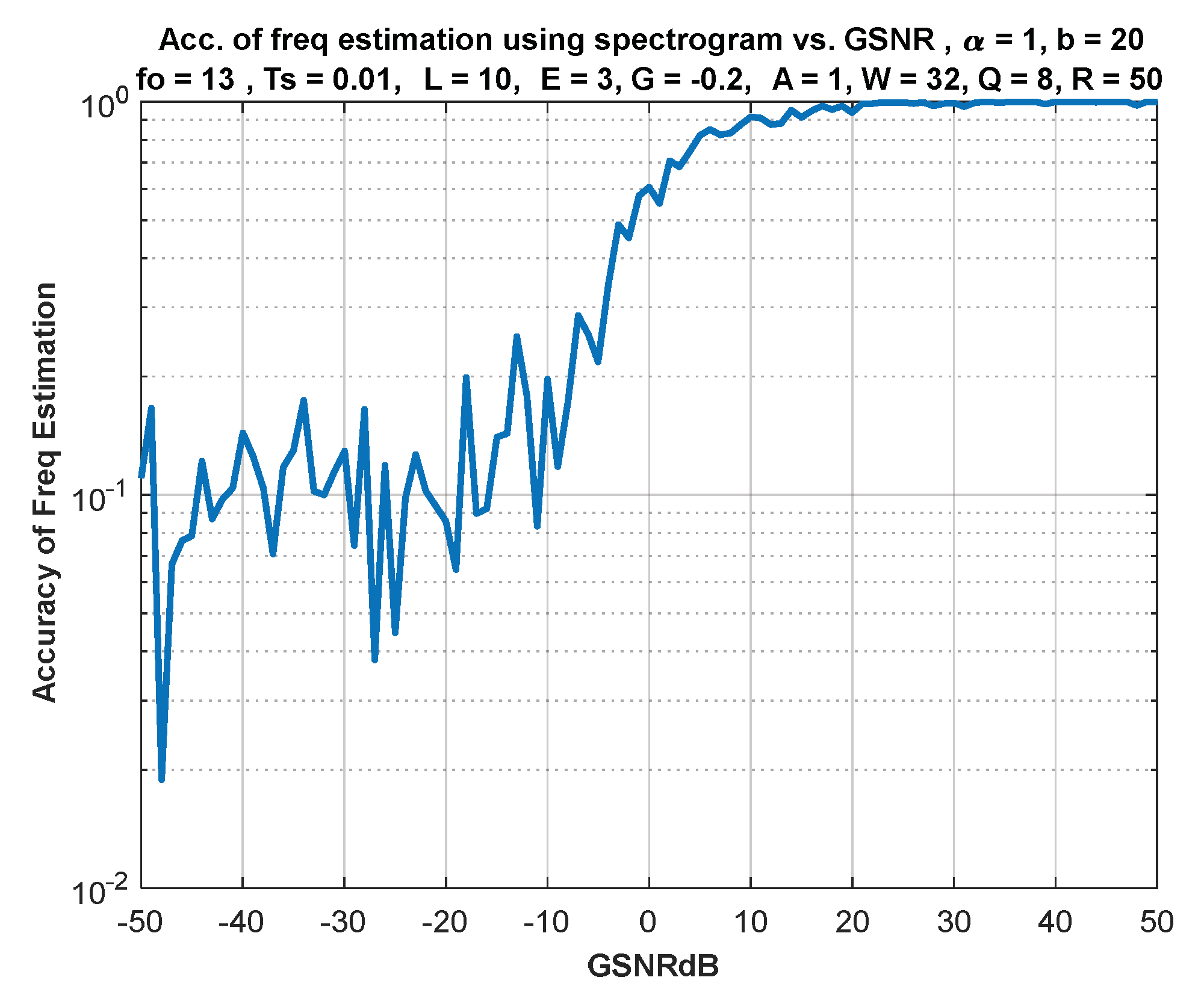
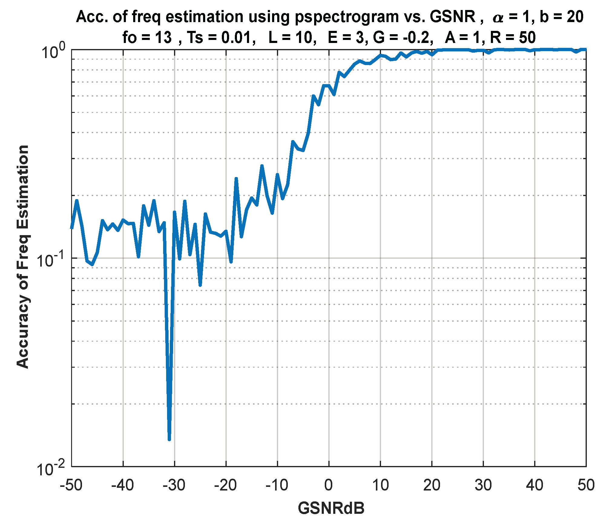
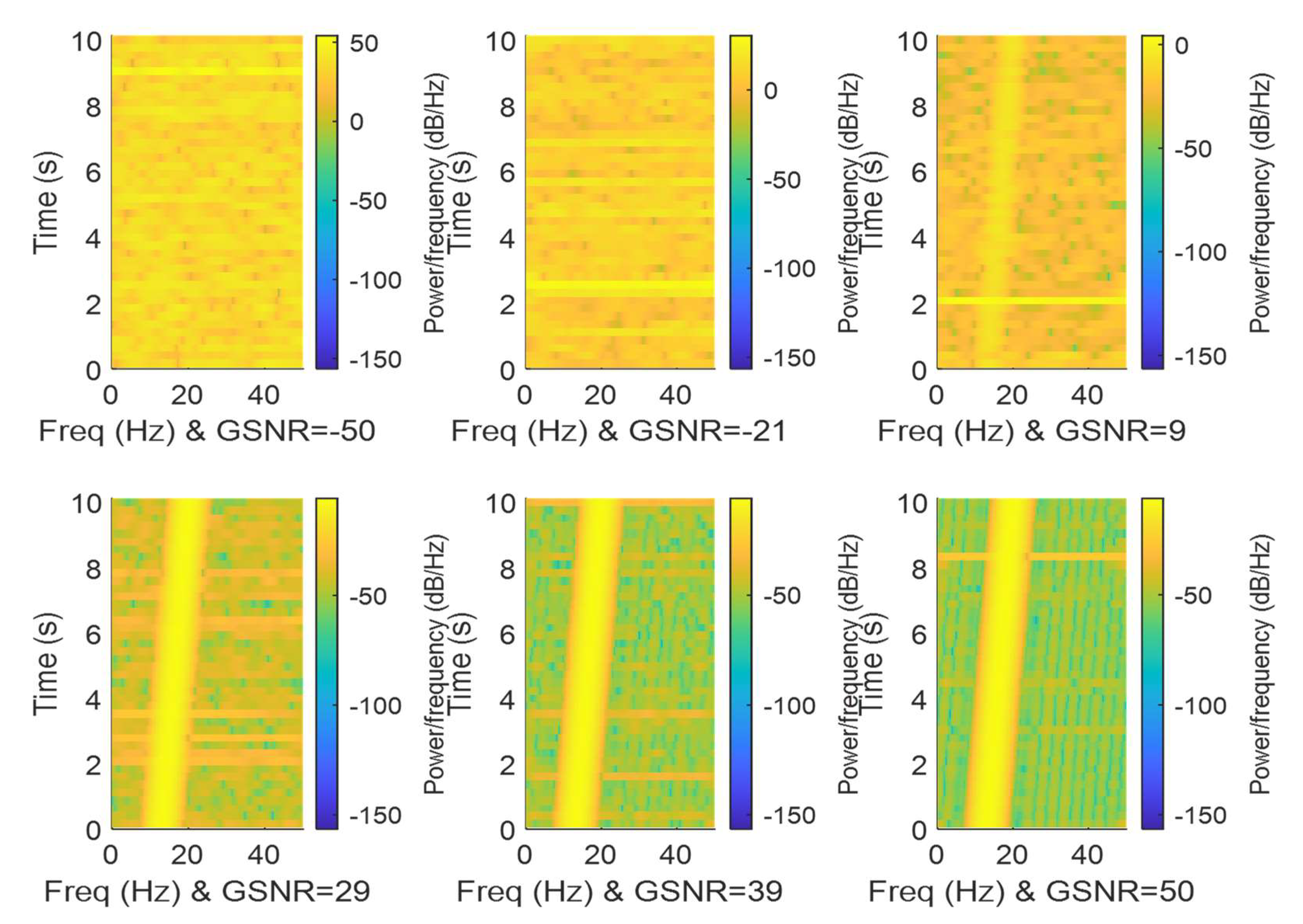
6. IF Estimation Based on TFD

The Fourier transform cannot detect the time-varying properties of nonstationary signals with time-varying frequency content (such as FM and bio-logical signals). This is due to the FT’s use of a time-averaging process (time integration). TFDs are two dimensional double transforms from the time domain to the time–frequency domain representing the Fourier transform of an analytical signal’s instantaneous autocorrelation. The most straightforward formula for a time–frequency distribution is the short-time Fourier transform (STFT), which is a windowed frequency distribution [27,28]. STFT is a sequence of Fourier transforms of a windowed signal; it is used to determine the sinusoidal frequency of local sections of a signal as it changes over time. STFTs divide a longer time- signal into segments of equal length and then compute the Fourier transform separately on each segment. A nonstationary signal is one with a changing frequency content over time. A nonstationary signal’s spectrogram estimates its frequency content’s time evolution. TFD IF estimation in the presence of noise AWGN and SαSN in FM signals. TFD and STFT are used to estimate the IF for analytical signals. Before frequency calculation, the analytic noisy signal is computed by using the Hilbert transformation. A real-valued signal’s Fourier Transform (FT) is complex and symmetric. This implies that the content at negative frequencies is superfluous. Negative frequencies may cause aliasing while analyzing FM. The analytic signal helps avoid aliasing. Although the analytic signal is complex valued, its spectrum is unipolar (only positive frequencies). The real part of the analytic signal is the original signal, and the imaginary part is the signal’s Hilbert Transform (HT). To pass complex-valued data to a neural network, you can use the input layer to split the complex values into their real and imaginary parts before it passes the data to the subsequent layers in the network. See reference [29].
We calculate the spectrogram of STFT ( spec t . f ), then estimate the IF from the peak (max) of the spec as follows:
f ^ = arg max spec t , f , 0 f f s 2
Then, we calculate the relative squared error for each GSNR as follows:
e = f ^ × d f IF t / f o 2
where f o fundamental frequency, f ^ estimated frequency, IF t theoretical IF with spectrogram timing, d f = f s N and N = 1024 . TFD estimated IF using spectrogram and pspectrum MATLAB functions, pspectrum differs from spectrogram in segment lengths, overlapping segments, and window. Spectrogram length = 1 × N 2 + 1 , while pspectrum length = 1 × N . Pspectrum controls the length of the segments and the overlap between adjacent segments using the time resolution and overlap percent pair arguments. It divides the signal into overlapping segments and applies a Kaiser window to each segment.
The algorithms (4, 5, and 6) illustration frequency estimation by TFD, Hilbert transform, and spectrogram by short time Fourier transform respectively as shown in Appendix C.

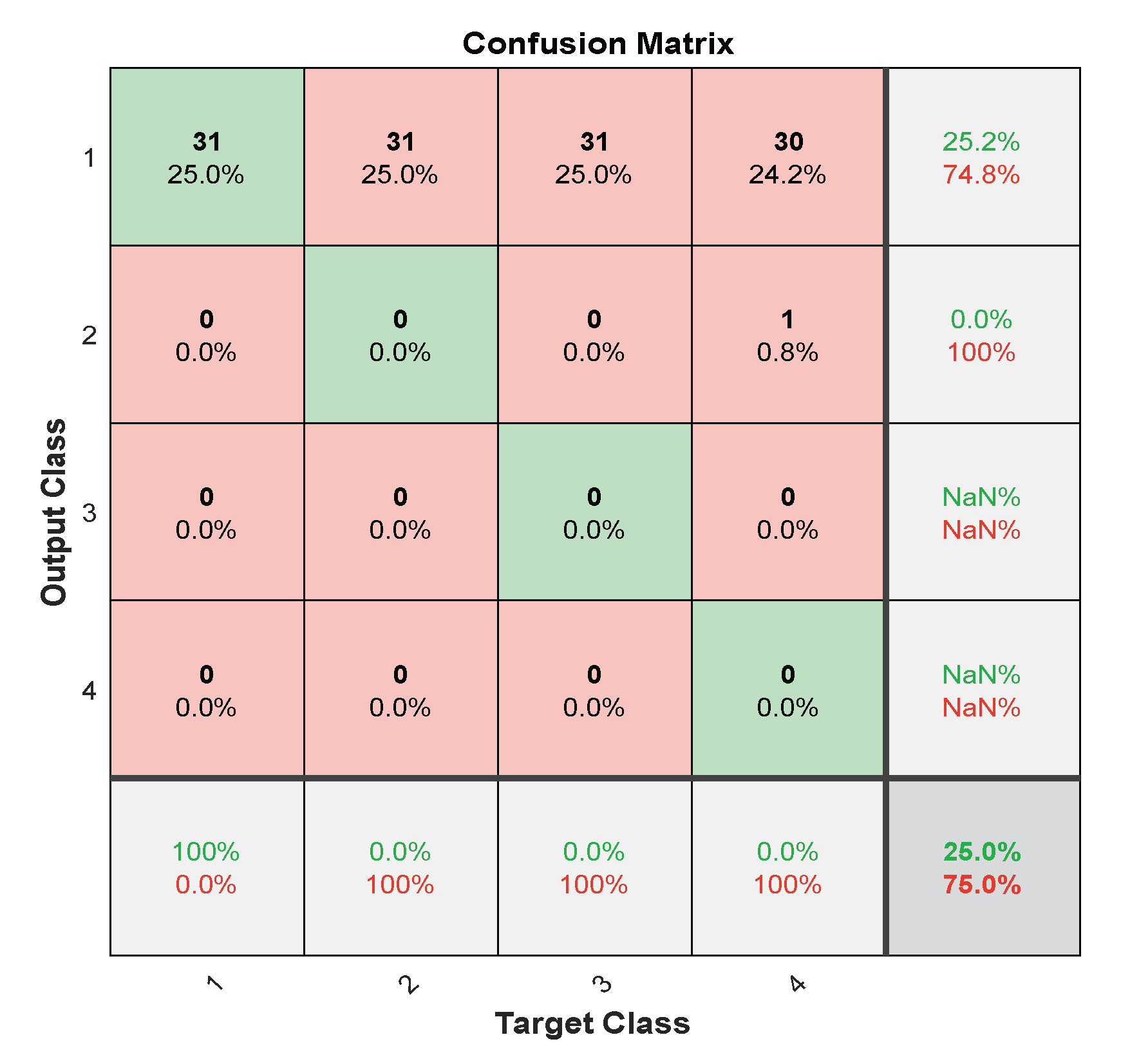
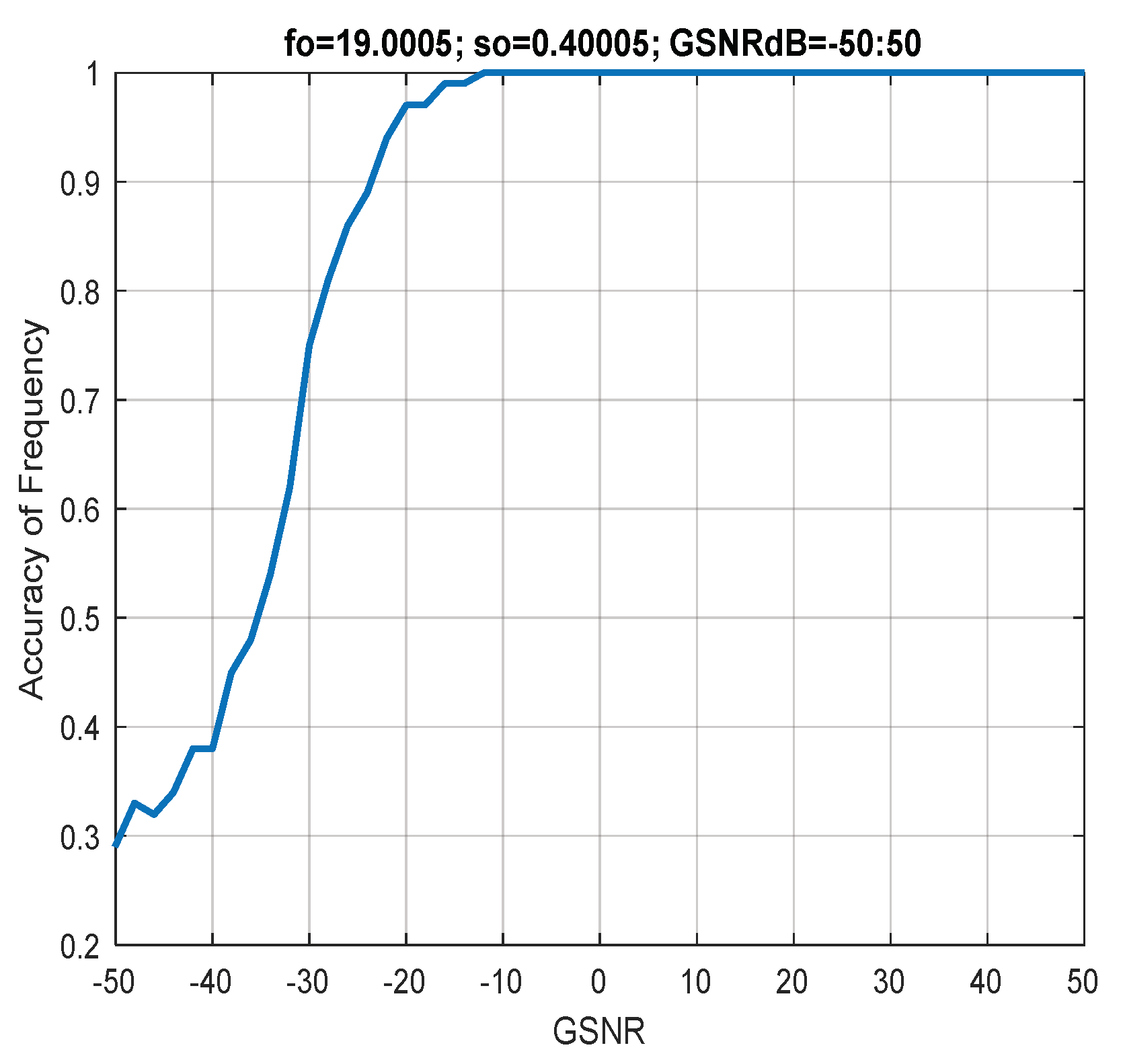
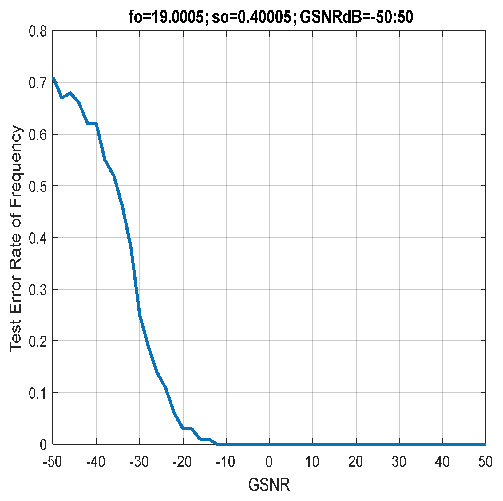
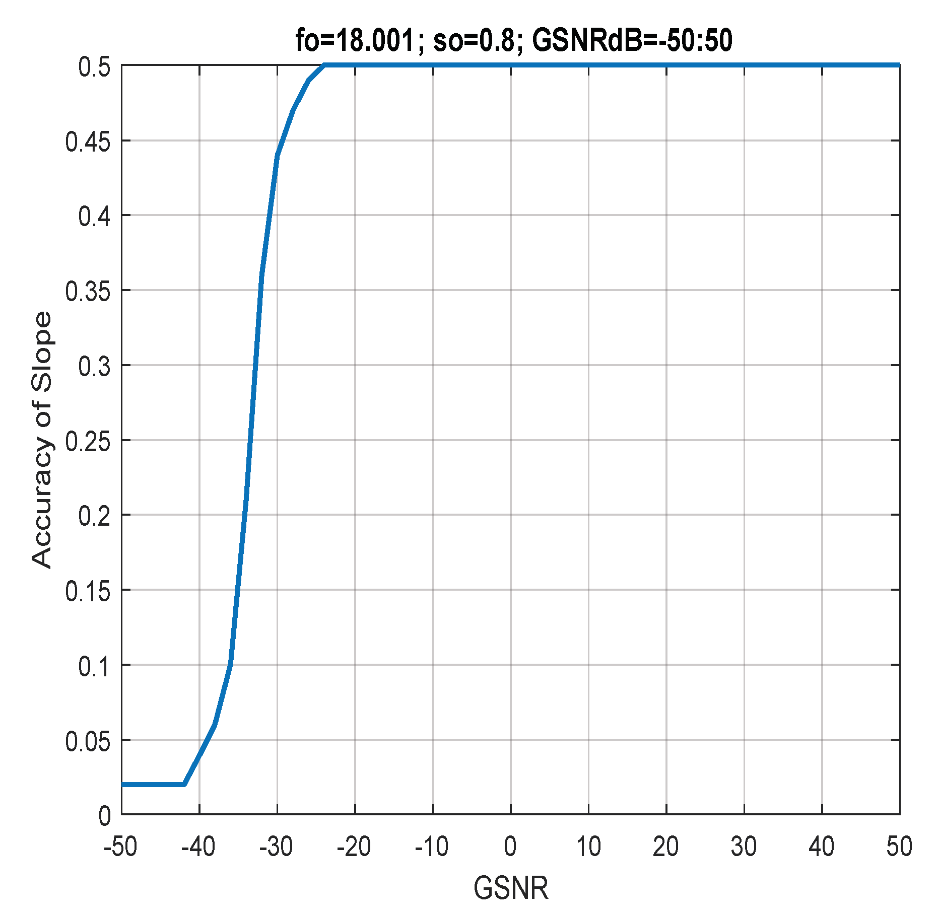
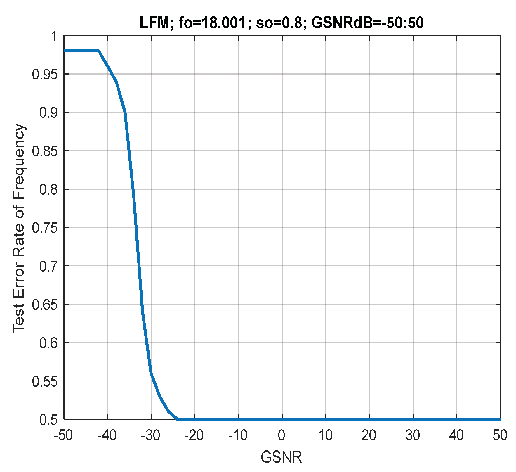
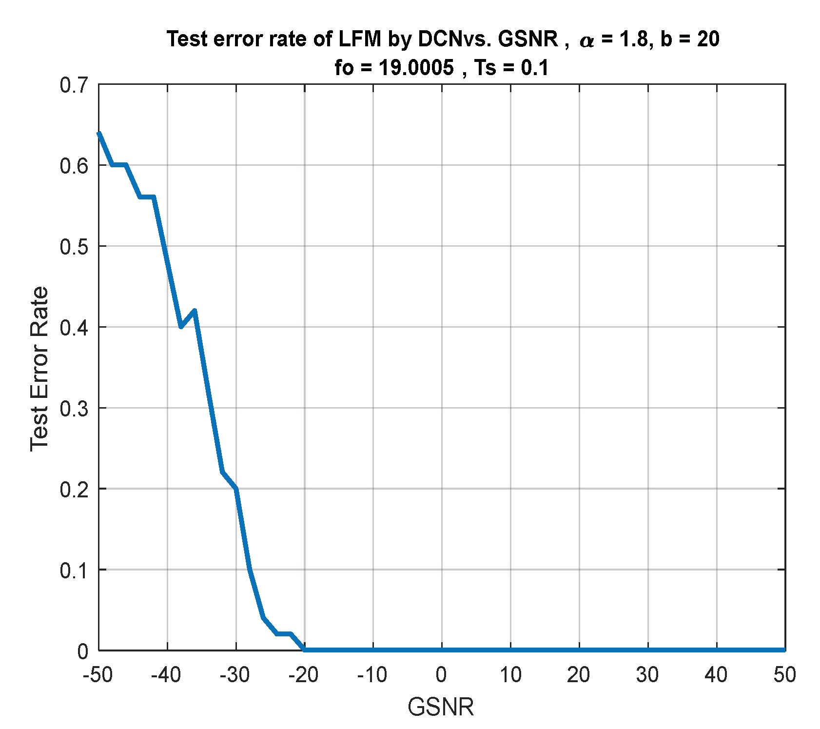
7. Discussion of Results

This section simulates the instantaneous frequency and slope estimation of FM signals using additive white Gaussian noise and symmetric stable noise. Simulation was performed with MATLAB under Academic License 40635944. [−50 50] dB is the GSNR range. The network learns from the input data and predicts the frequency and slope. The DNN and CNN models were used to simulate frequency and slope estimation for LFM signals. The results show high accuracy for parameter estimation by confusion matrix and some measures such as accuracy, precision, F1-score, FNR, FPR, and ROC, as well as few errors rate, and SαS is an impulsive model, where alpha is more harmful even if it is of small value, where it affects the slope and frequency guess. A variable b determines the ratio of AWGN and SαSN.
Figure 11 shows α-stable probability density functions with different parameters. Figure 12 shows alpha-stable noise in the time domain; it is impulsive. Figure 13 shows single-tone and noise signals. Figure 14 and Figure 15 show frequency estimation of single-tone (ST) and LFM signals by DNN. Figure 16 shows the slope estimation of single-tone and LFM signals by DNN. Figure 17 show the accuracy and loss rate of FE and SE for noisy LFM. Figure 18 show confusion matrices for FE and SE for noisy LFM. Figure 19 show the accuracy and loss rate of FE and SE for noisy LFM. Figure 20 show confusion matrices for FE and SE for noisy LFM. Table 1 and Table 2 show the performance evaluation criteria of noisy LFM signals. Figure 21 shows the accuracy of the frequency estimation of LFM. Figure 22 shows the test error of frequency estimation for LFM. Figure 23 shows the accuracy of the slope estimation of LFM. Figure 24 shows the test error of slope estimation for LFM. Figure 25 and Figure 26 show MSE versus GSNR for TFD of a noisy single-tone signal by spectrogram and pspectrum, where α = 1 and b = 20. Figure 27 and Figure 28 show MSE versus GSNR for TFD of noisy LFM signal by spectrogram and pspectrum, where α = 1 and b = 20. Figure 29 and Figure 30 show the accuracy of FE for noisy single tone and LFM signals by TFD (pspectrum). Figure 31 shows the accuracy of FE for noise LFM by DNN and TFD (spectrogram and pspectrum). Figure 32 shows the test error of FE for noisy LFM by DNN and TFD (spectrogram and pspectrum). Figure 33 shows the test error rate for SE of noisy LFM by CNN, where f o = 19.0005 . Figure 34 shows ROC for noisy LFM by 2D-CNN. Figure 35 shows ROC for noisy LFM by 2D-CNN, where the epoch number equals 30. Table 3 shows measures of the 1D-CNN model for noisy LFM signals. Figure 36 shows ROC for noisy LFM by 1D-CNN. Figure 37 signals in the time domain with different frequencies, LCR, and GSNR. Figure 38 shows 2D-signals in the time domain with different initial frequencies. Figure 39 shows signals in time frequency distribution.
Table 1 and Table 2 show the differences between implementing a 1D-CNN and 2D-CNN. Table 3 shows the training parameters of the noisy LFM dataset. Because the classification accuracy in a one-dimensional convolutional network is very low, the guess of parameters is influenced. The lower error of the slope and frequency estimation refers to the higher accuracy of the classification and the rest of the measures. The measures are used to evaluate the efficiency of the CNN model. If these measurements have high values, we can conclude that the slope and frequency estimations are correct. ROC scale is used to test the effectiveness of the CNN model (as shown in Figure 34, Figure 35 and Figure 36).
The results show that deep neural networks are better than time–frequency distribution for estimating the instantaneous frequency, and CNN is better than deep neural networks in estimating the instantaneous frequency of nonstationary signals. For time–frequency distribution, spectrogram and pspectrum functions have been used, where the results show that pspectrum is better than spectrogram for the IF estimate.
Further inspection of Figure 31 and Figure 32 reveals that the performance of CNN (in terms of accuracy) can give acceptable results at very low signal-to-noise ratios where TFD fails, giving more than 20 dB difference in the GSNR working range as compared to the classical spectrogram-based estimation. Considering more advanced (though more complex) methods of LFM instantaneous frequency estimation such as Viterbi-based approach [30] and fractional Fourier transform-based approach [31], the performance of CNN gives more than 15 dB difference (please compare with Figure 3 in [30], knowing that reference [30] considers only Gaussian noise. In contrast, this work finds the much more damaging α-stable noise.
Future Directions: It should be noted that this research considers only mono-component linear FM signals. Future directions may consider multicomponent signals and non-linear FM, where more advanced time–frequency distributions would be used instead of the spectrogram of Equation (23) [32,33,34]. As we only considered mono-component LFM signals in this work, the spectrogram and Wigner–Ville distribution (WVD) are the widely used FE methods, where the spectrogram is chosen as per Equation (23) as it behaves better under noise than WVD due to the fact that it does not suffer from the cross-term effect [32,34]. In addition, as compressive sensing is a promising technology for sensors, wireless sensor networks (WSNs), and IoT applications [35], this research can be further enhanced by considering frequency estimation from compressed measurements [36].

8. Further Remarks

We will highlight some points in the proposed network prediction.

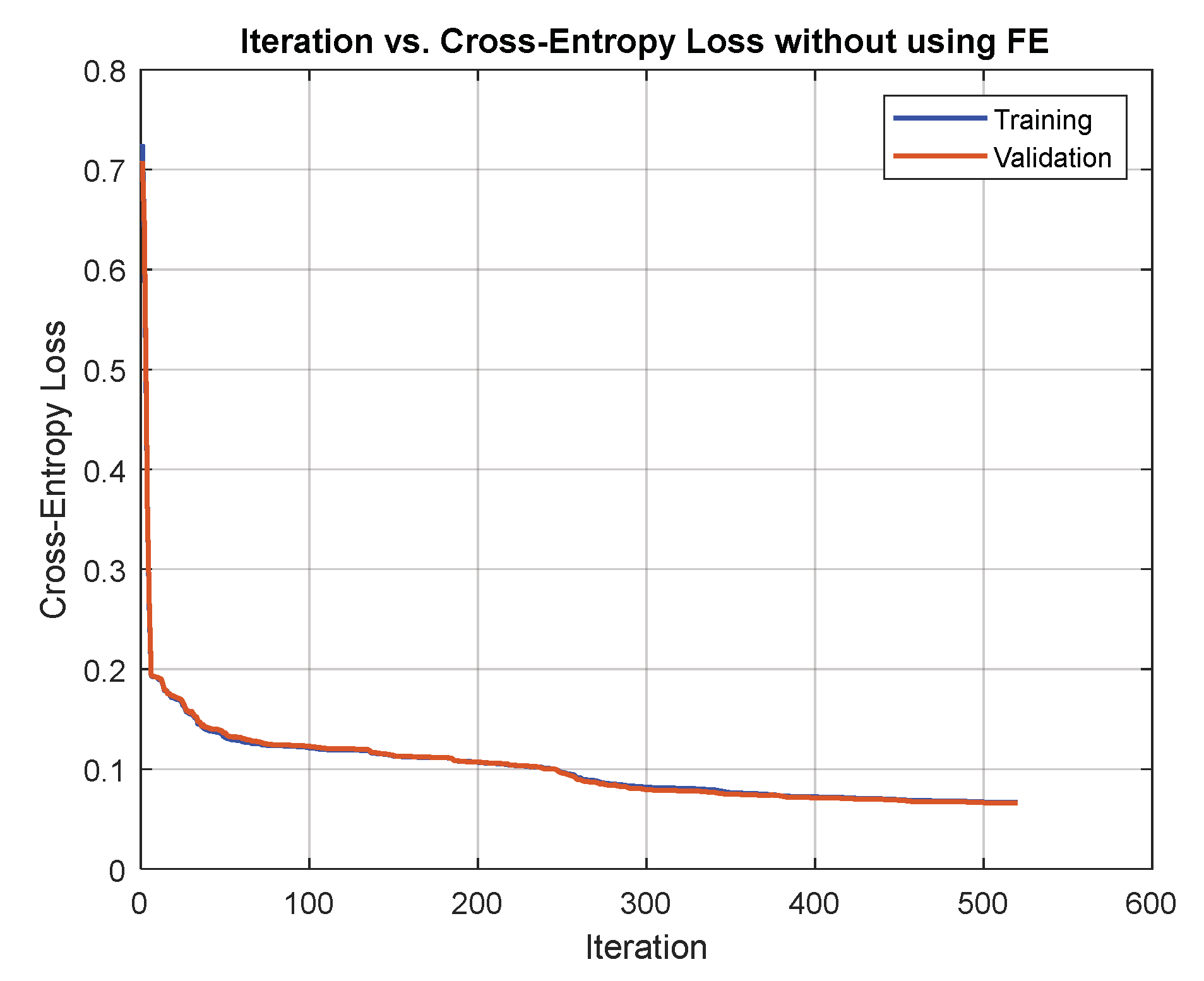
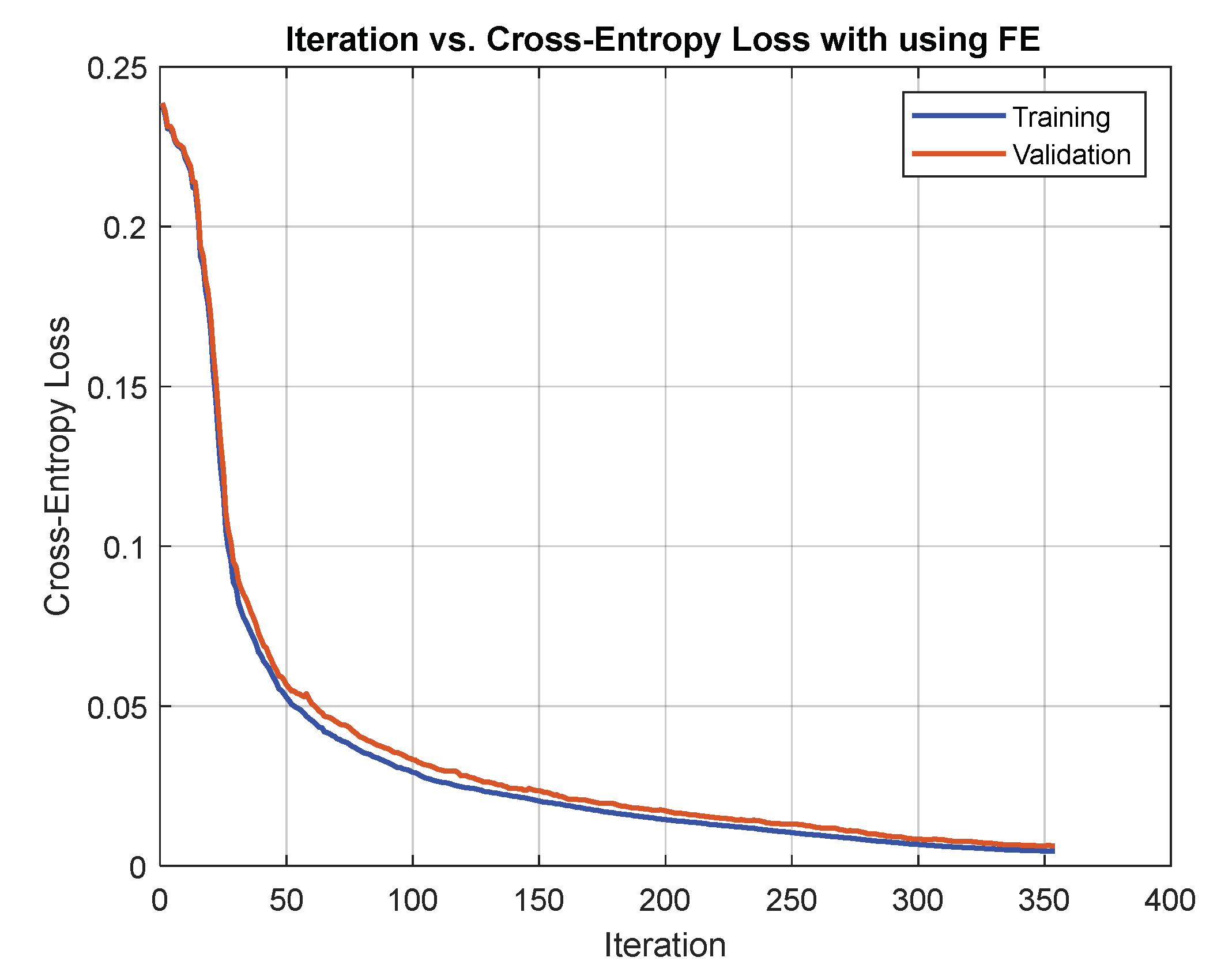
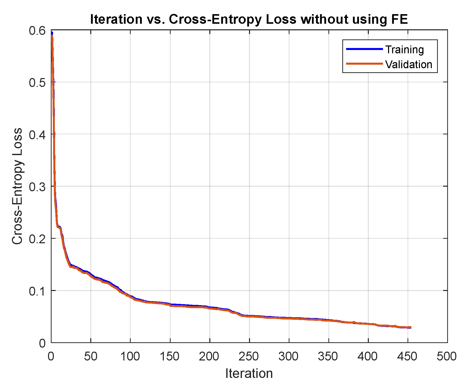
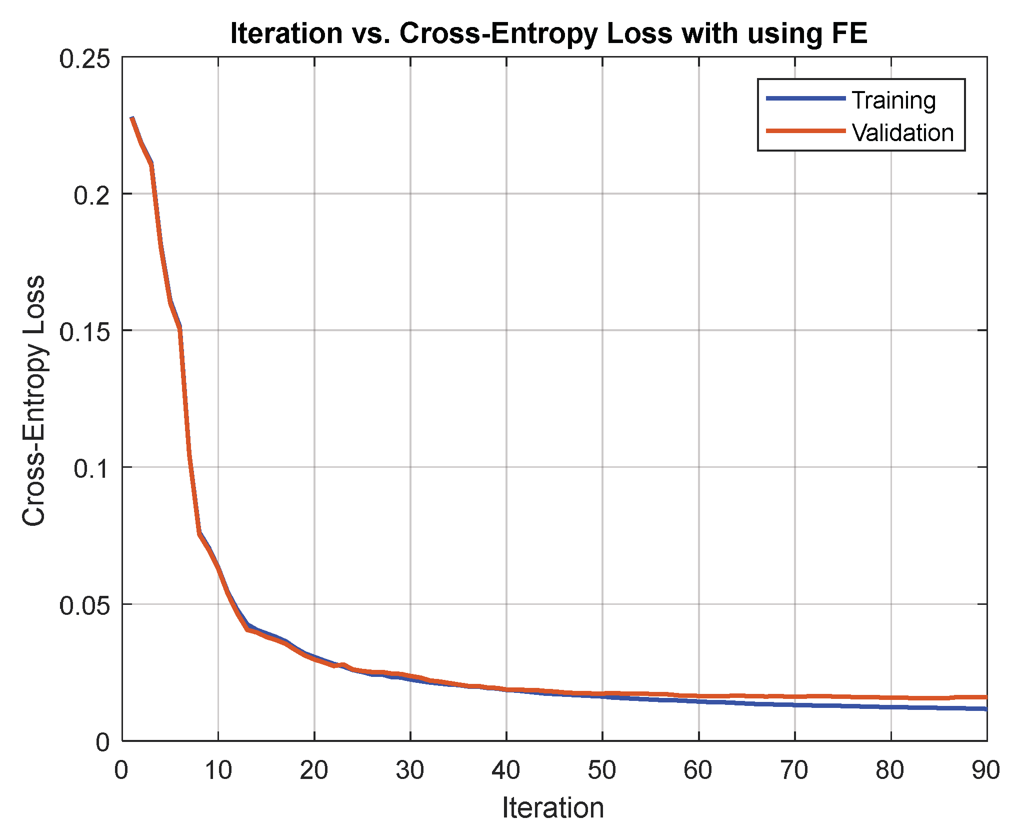
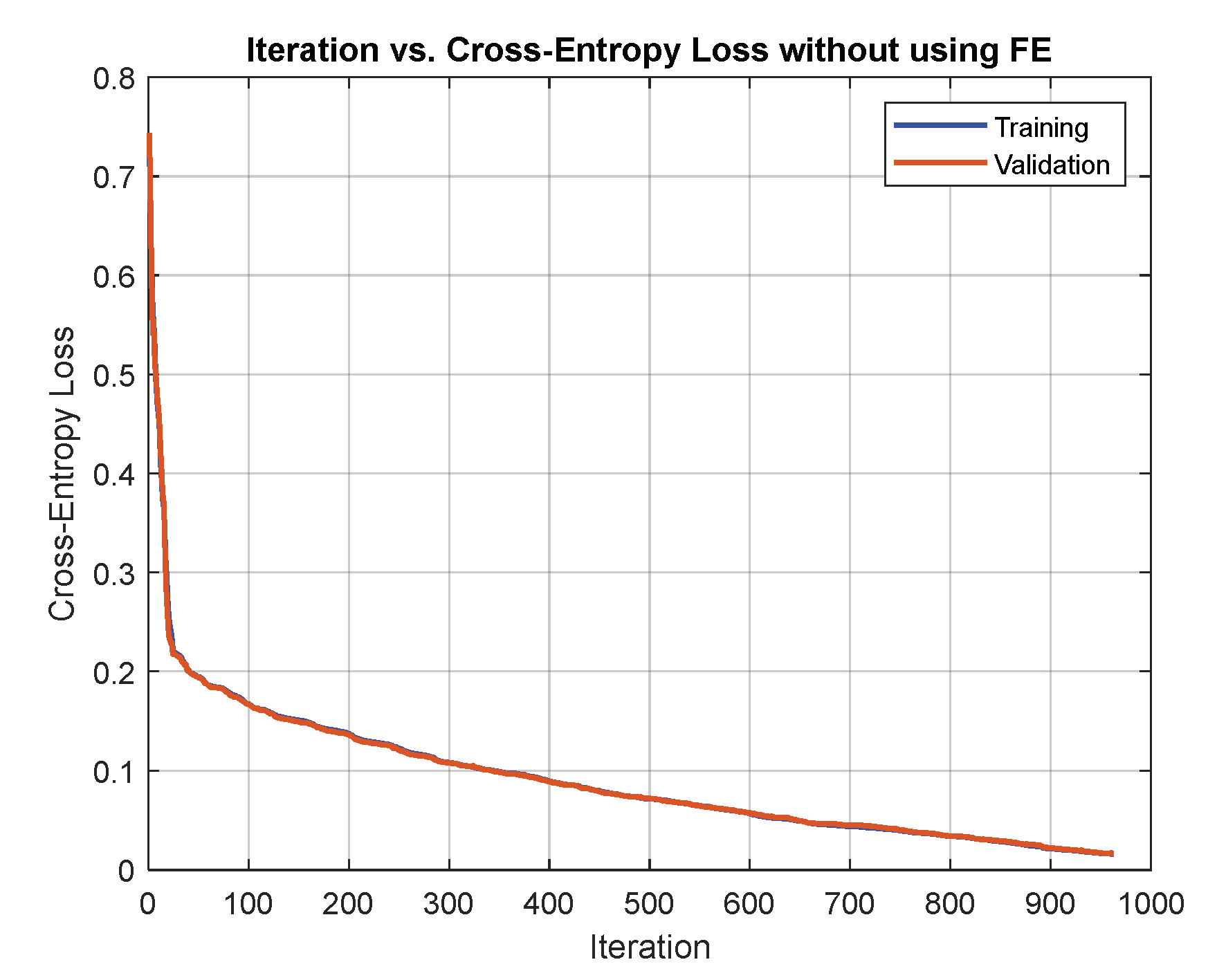
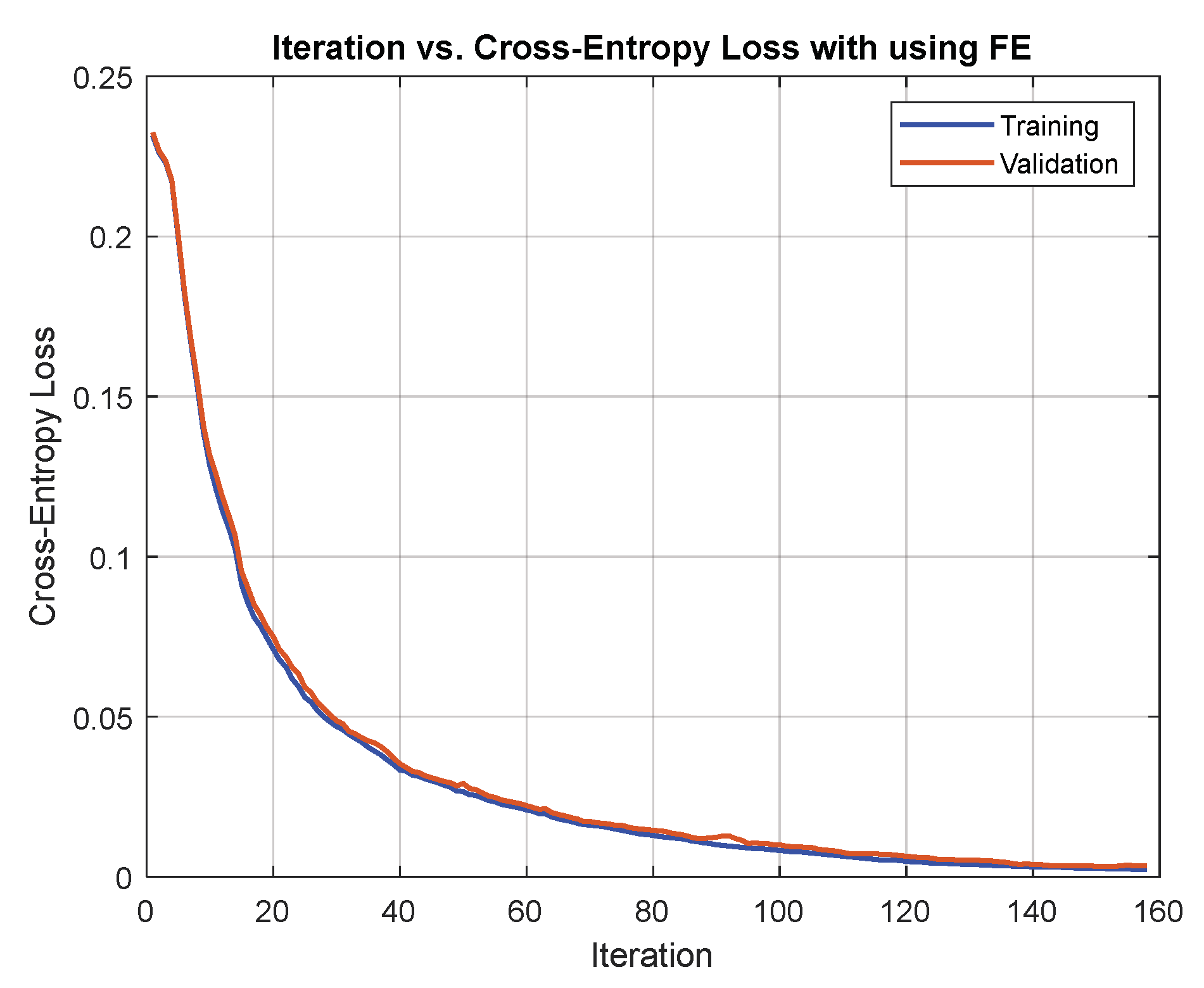
8.1. Comparing Network Training with and without Extracted Features

From Figure 31 and Figure 32, we conclude that extracting the features of the noisy input signals significantly reduces the error rate and increases the system’s accuracy. Thus, this affects the estimation of slope and frequency. A previously trained CNN model extracted the features. The CNN model was used to extract the features and classification as described in Section 5.4. The CNN model has two functions, which are feature extraction and classification. The parameters were estimated by extracting the features from the pre-trained CNN model and predicting parameters using simple DNN, which consists of one hidden layer containing ten nodes, ReLU activation function for the hidden layer, and softmax activation function for the output layer. Note the increasing number of iterations when DNN is trained without feature extraction.

8.2. Different Lengths for the Input Signal and Feature Vector

From Figure 33 and Figure 34, we conclude that the input length also affects the neural network. If the input is a noisy signal with a large number of samples (size), it would be difficult for the network to work with high accuracy, especially if the network structure is simple. Then when reducing the length of such signals, the accuracy improves. Reducing the features has the opposite effect. That is the fewer features, the lower the accuracy. DNN consists of one hidden layer containing ten nodes, a ReLU activation function for the hidden layer, and a softmax activation function for the output layer. Note that decreasing the length of input signals leads to better accuracy and less time, but reducing the size of input features leads to less accuracy and less time.

8.3. Effect of Network Training by the Number of Layers and Number of Nodes

The number of hidden layers and the number of nodes per layer play significant roles in deciding the speed and accuracy of neural networks. Figure 35 and Figure 36 illustrates the effect of the network structure on the prediction results, where the network performance improves when a specific number increases the number of hidden layers. In contrast, an excessive increase may lead to negative results. DNN consists of three hidden layers containing (30, 25, and 20) nodes, ReLU activation function for hidden layers, and softmax activation function for the output layer.

9. Conclusions

This paper provided an overview of the performance of machine learning and deep learning approaches for estimating the frequency and slope of a noisy LFM signal. Under additive white Gaussian noise and symmetric α-stable noise, the simulation is a relevant signal (impulsive model). This work solves problems using traditional, machine, and deep learning approaches. It examines the frequency and slope estimation error under various GSNRs. In DNN, only two hidden layers are used. The convolution layer, ReLU activation function, max-pooling layers, dropout layer, fully connected layer, softmax layer, and classification layer are the 19 layers used in the CNN model. The simple structure designed for the DNN or CNN model works to reduce the communication system’s complexity, power consumption, and cost. These characteristics are advantageous for systems with limited memory and computational processes, such as WSNs, which connect to the internet of things applications. The simulation results show that alpha is more harmful than beta, even if it has a small incapacity, and it significantly affects guess frequency and slope. CNN was used to estimate the parameters of LFM signals in this paper. Future research will focus on compressed and multicomponent non-linear FM signals.

Author Contributions

H.S.R. and Z.M.H. contributed equally to this work. H.S.R. contributed to the initial tasks of this work during her postgraduate preparatory year of coursework in 2019, where she obtained the top rank of high distinction before she started her research project on deep learning for frequency estimation under the supervision of Z.M.H. All authors have read and agreed to the published version of the manuscript.

Funding

This project was partially funded by Edith Cowan University via the ASPIRE Program.

Institutional Review Board Statement

Not applicable.

Informed Consent Statement

Not applicable.

Data Availability Statement

All types of data were generated using mathematical equations.

Acknowledgments

The authors would like to thank Edith Cowan University for partially supporting this project. Thanks are extended to the (anonymous) reviewers for their constructive comments that improved this paper.

Conflicts of Interest

The authors declare that no conflict of interest is associated with this work.

Appendix A

The procedures of SαS are as follows:
  • For β = 0: symmetric α-stable noise Y can be generated as follows. A uniformly distributed random variable V and an independent exponential random variable W are generated as follows:
V   =   π 2 ·   2 U   1
W = log H
where U ,   H U , the standard uniform distribution. Then SαS for α 1 is obtained:
X = sin α · V { cos V } 1 / α · cos V · 1 α W 1 α / α
Y = γ X + μ
Moreover, SαS for α = 1 is obtained:
X = tan V
Y = γ X + μ .
2.
For α 1 , a uniformly distributed random variable V and an independent exponential random variable W are generated as follows to get X :
V   =   π ·   U   0.5
W = log H
X = S α , β · sin α V + B α , β { cos V } 1 / α · cos V α V + B α , β W 1 α / α
S α , β = 1 + β 2 tan 2 π α 2 1 / 2 α
B α , β = arctan β tan π α 2 α .
When scale and shift are applied, we have:
  Y = γ X + μ .
3.
For α = 1 , random variables V and W are generated as above, then:
  X = 2 π π 2 + β V tan V β log π 2 W cos V π 2 + β V
When scale and shift are applied as an equation, we have:
Y = γ X + 2 π β γ log γ + μ .

Appendix B

Table A1 shows the parameters description of CNN layers, where F S is filter size, N F is the number of filters (number of output feature maps), S is stride, P is padding, C is the number of channels (number of input feature maps), a total of parameters is number of weights plus number of biases; in batch normalization ε is epsilon, Β is sifted, λ is scale, T ρ is the total number of parameters in a convolutional layer, and bias b = 1:
T ρ = F S · F S · C + b · N F
Table A1. Topology of the proposed CNN model.
IndexesLayers NameInput SizeOutputSizeHyperparametersTotal of Parameters
1.Image Input80 × 80 × 180 × 80 × 1Normalization zero-center0
2.Convolution 80 × 80 × 180 × 80 × 30 F S = 3 × 3 ,
N F = 30 ,   S = 1 ,  
P = 1 ,   C = 1
300
3.Batch Normalization80 × 80 × 3080 × 80 × 30 ε =0, Β =0, λ =10
4.ReLU80 × 80 × 3080 × 80 × 30-0
5.Max Pooling80 × 80 × 3040 × 40 × 30 F S = 2 × 2 ,   S = 2 0
6.Convolution 40 × 40 × 3040 × 40 × 60 F S = 3 × 3 ,
N F = 60 , S = 1 ,   P = 1 , C=30
16,260
7.ReLU40 × 40 × 6040 × 40 × 60-0
8.Max Pooling40 × 40 × 6020 × 20 × 60 F S = 2 × 2 ,   S = 2 0
9.Convolution20 × 20 × 6020 × 20 × 90 F S = 3 × 3 ,
N F = 90 ,   S = 1 ,   P = 1
48,690
10.ReLU20 × 20 × 9020 × 20 × 90-0
11.Max Pooling20 × 20 × 9010 × 10 × 90 F S = 2 × 2 ,   S = 1 0
12.Convolution10 × 10 × 9010 × 10 × 128 F S = 3 × 3 ,
N F = 128 ,   S = 1 ,   P = 1
103,808
13.ReLU10 × 10 × 12810 × 10 × 128-0
14.Max Pooling10 × 10 × 1285 × 5 × 128 F S = 2 × 2 ,   S = 1 0
15.Fully Connected5 × 5 × 128 = 3200100Nodes = 100320,100
16.Dropout--Probability = 0.50
17.Fully Connected10010No. class = 101010
18.Softmax1010-0
19.Classification101Loss Function = cross-entropy0
Number of weights for convolution layers = (270 + 16200 + 48600 + 103680) = 168750
Number of biases for convolution layers = (30 + 60 + 90 + 128) = 308
Total parameters for convolution layers = 169058
Total parameters for all network = 169058 + 320100+1010 = 490168

Appendix C

Algorithm A1: Frequency Estimation by TFD
Input: The   sin gle - tone   and   LFM   signals   x t .
Output: Instantaneous frequency estimate f ^ .
Begin:
Step 1: Initial   parameters   are   initial   frequency   f o = 23 ,   T s = 0.01 , f s   =   1 T s ,   f s 2   =   f s 2 ,   d f   =   f s N ,   f 1   =   0     d f     f s 2 , and   N = 1024 .
Step 2: Geometric   SNR   vector   ( s r ) ,   s r   50   50 ,   number   of   realizations   R = 50 , the duplicate input signal in R rows, may repeat run R times to get a good result.
Step 3: For   m   =   1 s r
   ● The S α S noise ( Y ) and Gaussian noise ( G ) are generated as above explained.
   ● The input signals are corrupted by hybrid noise, where total noise ( N T ) is a mixture of both Gaussian noise and S α S noise:
N T = G + Y
y t = x t + N T

   ● IF error temporary matrix, where E   =   zeros   (initially).
Step 4: For   h = 1 : R
  ■ Take hth realization, where z   =   y h .
  ■ Eliminate the negative portion of the signal spectrum by called Alg. (5) with an input parameter ( z ) and an output parameter S A .
  ■ IF estimate with spectrogram and pspectrum by called Alg. (6) with input parameter S A and output parameter spec t ,   f :
  ■ Estimate the IF from the peak (max) of the s p e c t ,   f as follows:
f ^ = max spec t , f

  ■ Calculate the relative squared error for each GSNR:
e = f ^ × d f I F t f o 2
E = E + e

where   IF t theoretical instantaneous frequency.
  ■ End of h loop
Step   6 :   IF   estimation   error   at   GSNR   dB ,   where   F E m   = E R
End of m loop
End of algorithm
Algorithm A2: Hilbert Transform
Input :   The   signal   z t .
Output :   Analytic   signal   S A t .
Begin:
Step   1 :   Compute   the   FFT   of   the   signal   z t   to   give   spectrum   Z f .
Step   2 :   Creates   a   vector   h   whose   elements   h i have three values as follows:
h i = 1         if   i   =   1   o r   n 2 + 1 2         if     i   =   2 ,   3 ,     , n 2 0         if   i   =     n 2 + 2 ,     ,   n
    where n = Z .
Step   3 :   Find   signal   ( m s ) ,   where   m s = Z × h .
Step   4 :   Compute   ( S A ) by   inverse   FFT   of   vector   m s , where S A = IFFT m s
End of algorithm
Algorithm A3: Spectrogram of Short-Time Fourier Transform
Input: Analytic signal S A t and N =   S A t .
Output: Spectrogram spec t ,   f , time and frequency vectors t ,   f .
Begin:
Step 1: Define the parameters of STFT are window length m , hop size h , window overlap q , sampling frequency ( f s ), and the number of FFT points nfft .
Step 2: Create Hamming window win of length m = 32 ,   q = m 4 , and h = m q .
Step 3: STFT matrix S with size NUP ,   L , where L is the number of signal frames.
NUP =   nfft
L = N q h

Step 4: Divides the input signal S A t into overlapping segments and multiply each segment by the window ( S w ) . Then fast Fourier transform is applied to each segment ( S w ) :
For i   =   0 L 1
S w   =   S A i h + 1     i h o p + m   w i n
X   =   F T S w
S : ,   i + 1   =   X 1 N U P

End of i loop
Step 5: Find the spectrogram spec t ,   f , were
spec t ,   f = 2 win / N × S .

Step 6: Calculation of the time t vector in second and frequency f vector in H z , were
t = m 2 , m 2 + h , , m 2 + L 1 × h / f s
f = 0 , , NUP 1 × f s / nfft

End of algorithm

References

  1. Boashash, B. Estimating and interpreting the instantaneous frequency of a signal—I: Fundamentals. Proc. IEEE 1992, 80, 520–538. [Google Scholar] [CrossRef]
  2. Boashash, B. Estimating and interpreting the instantaneous frequency of a signal—II: Algorithms and applications. Proc. IEEE 1992, 80, 540–568. [Google Scholar] [CrossRef]
  3. Liu, J.; Fan, L.; Jin, J.; Wang, X.; Xing, J.; He, W. An Accurate and Efficient Frequency Estimation Algorithm by Using FFT and DTFT. In Proceedings of the 39th Chinese Control Conference (CCC), Shenyang, China, 27–29 July 2020. [Google Scholar]
  4. Akram, J.; Khan, N.A.; Ali, S.; Akram, A. Multi-component instantaneous frequency estimation using signal decomposition and time-frequency filtering. Signal Image Video Process. 2020, 14, 1663–1670. [Google Scholar] [CrossRef]
  5. Xu, S.; Shimodaira, H. Direct F0 Estimation with Neural-Network-Based Regression. In Proceedings of the INTER-SPEECH, Graz, Austria, 15–19 September 2019; pp. 1995–1999. [Google Scholar]
  6. Silva, B.; Habermann, D.; Medella, A.; Fraidenraich, G. Artificial Neural Networks to Solve Doppler Ambiguities in Pulsed Radars. In Proceedings of the International Conference on Radar (RADAR), Brisbane, Australia, 27–31 August 2018; pp. 1–5. [Google Scholar]
  7. Chen, X.; Jiang, Q.; Su, N.; Chen, B.; Guan, J. LFM Signal Detection and Estimation Based on Deep Convolutional Neural Network. In Proceedings of the Asia-Pacific Signal and Information Processing Association Annual Summit and Conference (APSIPA ASC), Lanzhou, China, 18–21 November 2019; pp. 753–758. [Google Scholar]
  8. Xuelian, L.; Wang, C. A novel parameter estimation of chirp signal in α-stable noise. IEICE Electronics Express 2017, 14, 20161053. [Google Scholar]
  9. Aboutanios, E.; Mulgrew, B. Iterative frequency estimation by interpolation on Fourier coefficients. IEEE Trans. Signal Process. 2005, 53, 1237–1241. [Google Scholar] [CrossRef]
  10. Ahmet, S. Fast and efficient sinusoidal frequency estimation by using the DFT coefficients. IEEE Trans. Commun. 2018, 67, 2333–2342. [Google Scholar]
  11. Li, L.; Qiu, T. A Robust Parameter Estimation of LFM Signal Based on Sigmoid Transform Under the Alpha Stable Distribution Noise. Circuits Syst. Signal Process. 2019, 38, 3170–3186. [Google Scholar] [CrossRef]
  12. Almayyali, H.; Hussain, Z. Deep Learning versus Spectral Techniques for Frequency Estimation of Single Tones: Reduced Complexity for Software-Defined Radio and IoT Sensor Communications. Sensors 2021, 21, 2729. [Google Scholar] [CrossRef]
  13. Boashash, B. (Ed.) Time-Frequency Signal Analysis and Processing: A Comprehensive Reference, 2nd ed.; Elsevier: Oxford, UK, 2016. [Google Scholar]
  14. Milczarek, H.; Leśnik, C.; Djurović, I.; Kawalec, A. Estimating the Instantaneous Frequency of Linear and Nonlinear Frequency Modulated Radar Signals—A Comparative Study. Sensors 2021, 21, 2840. [Google Scholar] [CrossRef]
  15. Boashash, B.; O’Shea, P.; Arnold, M.J. Algorithms for Instantaneous Frequency Estimation: A Comparative Study; SPIE: Bellingham, WA, USA, 1990. [Google Scholar]
  16. Zhang, J.; Li, Y.; Yin, J. Modulation classification method for frequency modulation signals based on the time–frequency distribution and CNN. IET Radar Sonar Navig. 2018, 12, 244–249. [Google Scholar] [CrossRef]
  17. Liu, M.; Han, Y.; Chen, Y.; Song, H.; Yang, Z.; Gong, F. Modulation Parameter Estimation of LFM Interference for Direct Sequence Spread Spectrum Communication System in Alpha-Stable Noise. IEEE Syst. J. 2020, 15, 881–892. [Google Scholar] [CrossRef]
  18. Kristoffer, H. Symmetric Alpha-Stable Adapted Demodulation and Parameter Estimation. Master’s Dissertation, Lulea University of Technology, Lulea, Sweden, 2018. [Google Scholar]
  19. Braspenning, P.J.; Thuijsman, F.; Weijters, A.J.M.M. Artificial neural networks: An introduction to ANN theory and practice. In Lecture Notes in Computer Science; Springer Science & Business Media: Berlin/Heidelberg, Germany, 1995; Volume 931. [Google Scholar]
  20. Nwankpa, C.; Ijomah, W.; Gachagan, A.; Marshall, S. Activation functions: Comparison of trends in practice and research for deep learning. arXiv 2018, arXiv:1811.03378. [Google Scholar]
  21. Møller, M.F. A scaled conjugate gradient algorithm for fast supervised learning. Neural Netw. 1993, 6, 525–533. [Google Scholar] [CrossRef]
  22. Kingma, D.P.; Ba, J. Adam: A Method for Stochastic Optimization. arXiv 2014, arXiv:1412.6980. [Google Scholar]
  23. Yamashita, R.; Nishio, M.; Do, R.K.G.; Togashi, K. Convolutional neural networks: An overview and application in radiology. Insights Imaging 2018, 9, 611–629. [Google Scholar] [CrossRef] [PubMed] [Green Version]
  24. Moons, B.; Bankman, D.; Verhelst, M. Embedded Deep Learning: Algorithms, Architectures and Circuits for Always-on Neural Network Processing; Springer: Berlin/Heidelberg, Germany, 2018. [Google Scholar]
  25. Phil, K. Matlab Deep Learning with Machine Learning, Neural Networks and Artificial Intelligence; Apress: New York, NY, USA, 2017. [Google Scholar]
  26. Powers, D.M. Evaluation: From precision, recall and F-measure to ROC, informedness, markedness and correlation. arXiv 2011, arXiv:2010.16061. [Google Scholar]
  27. Hussain, Z.M.; Sadik, A.Z.; O’Shea, P. Digital Signal Processing: An Introduction with MATLAB and Applications; Springer: Berlin, Germany, 2011. [Google Scholar]
  28. Razzaq, H.S.; Hussain, Z.M. Instantaneous Frequency Estimation for Frequency-Modulated Signals under Gaussian and Symmetric α-Stable Noise. In Proceedings of the 31st International Telecommunication Networks and Applications Conference (ITNAC), Sydney, Australia, 24–26 November 2021. [Google Scholar]
  29. Gao, J.; Deng, B.; Qin, Y.; Wang, H.; Li, X. Enhanced radar imaging using a complex-valued convolutional neural network. IEEE Geosci. Remote Sens. Lett. 2018, 16, 35–39. [Google Scholar] [CrossRef] [Green Version]
  30. Djurović, I. Viterbi algorithm for chirp-rate and instantaneous frequency estimation. Signal Process. 2011, 91, 1308–1314. [Google Scholar] [CrossRef]
  31. Yin, Z.; Chen, W. A New LFM-Signal Detector Based on Fractional Fourier Transform. EURASIP J. Adv. Signal Process. 2010, 2010, 1–7. [Google Scholar] [CrossRef] [Green Version]
  32. Hussain, Z.M.; Boashash, B. Design of time-frequency distributions for amplitude and IF estimation of multicomponent signals. In Proceedings of the Sixth International Symposium on Signal Processing and its Applications (ISSPA2001), Kuala Lumpur, Malaysia, 13–16 August 2001. [Google Scholar]
  33. Nelson, D.J. Instantaneous Higher Order Phase Derivatives. Digit. Signal Process. 2002, 12, 416–428. [Google Scholar] [CrossRef]
  34. Yin, Q.; Shen, L.; Lu, M.; Wang, X.; Liu, Z. Selection of optimal window length using STFT for quantitative SNR analysis of LFM signal. J. Syst. Eng. Electron. 2013, 24, 26–35. [Google Scholar] [CrossRef]
  35. Hussain, Z.M. Energy-Efficient Systems for Smart Sensor Communications. In Proceedings of the IEEE 30th International Telecommunication Networks and Applications Conference (ITNAC), Melbourne, Australia, 25–27 November 2020. [Google Scholar]
  36. Alwan, N.; Hussain, Z. Frequency Estimation from Compressed Measurements of a Sinusoid in Moving-Average Colored Noise. Electronics 2021, 10, 1852. [Google Scholar] [CrossRef]
Figure 1. Iteration vs. cross-entropy loss for noisy signals with length 6400 and one hidden layer with ten nodes for DNN. Note that the error is higher than in Figure 32 and has less accuracy at 74 with more than 500 iterations.
Information 14 00018 g001
Figure 2. Iteration vs. cross-entropy loss for features extraction of noisy signals with length 6400, one hidden layer with ten nodes for DNN.
Information 14 00018 g002
Figure 3. Iteration vs. cross-entropy loss for noisy signals with length 1600, and one hidden layer with ten nodes for DNN.
Information 14 00018 g003
Figure 4. Iteration vs. cross-entropy loss for features extraction of noisy signals with length 1600 and one hidden layer.
Information 14 00018 g004
Figure 5. Iteration vs. cross-entropy loss for noisy signals with length 6400 and three hidden layers with (30, 25, and 20) nodes. Note that increased layers and nodes lead to increased accuracy of 96 and more iterations of 963.
Information 14 00018 g005
Figure 6. Iteration vs. cross-entropy loss for features extraction of noisy signals with length 6400 and three hidden layers with (30, 25, 20) nodes. Note that increased layers and nodes lead to an accuracy of 98 with fewer iterations of 158.
Information 14 00018 g006
Figure 7. GSNR vs. RMSE of FE for noisy LFM by DNN.
Information 14 00018 g007
Figure 8. ROC of FE for noisy LFM by DNN.
Information 14 00018 g008
Figure 9. A confusion matrix for noisy LFM by DNN.
Information 14 00018 g009
Figure 10. Proposed CNN model layers.
Information 14 00018 g010
Figure 11. α-Stable probability density functions with different parameters.
Information 14 00018 g011
Figure 12. α-Stable noise in time domain. It is impulsive.
Information 14 00018 g012
Figure 13. A single tone and noise signals.
Information 14 00018 g013
Figure 14. FE of noisy single tone signals by DNN.
Information 14 00018 g014
Figure 15. Error rate for FE of noisy LFM signals by DNN.
Information 14 00018 g015
Figure 16. Error rate for SE of noisy LFM signals by DNN.
Information 14 00018 g016
Figure 17. Accuracy and loss rate of FE for noisy LFM by CNN.
Information 14 00018 g017
Figure 18. A confusion matrix of FE for LFM signals by CNN.
Information 14 00018 g018
Figure 19. Accuracy and loss rate of SE for noisy LFM by CNN.
Information 14 00018 g019
Figure 20. A confusion matrix of SE for LFM.
Information 14 00018 g020
Figure 21. Accuracy of FE for noisy LFM by CNN, where f o = 19.0005.
Information 14 00018 g021
Figure 22. Test error rate of FE for noisy LFM by CNN, where f o   =   19.0005 .
Information 14 00018 g022
Figure 23. Accuracy of SE for noisy LFM by CNN, where f o = 18.001.
Information 14 00018 g023
Figure 24. Test error rate for SE of noisy LFM by CNN, where f o = 18.001.
Information 14 00018 g024
Figure 25. MSE versus GSNR for TFD of noisy single tone signal by spectrogram, where α = 1 and b = 20.
Information 14 00018 g025
Figure 26. MSE versus GSNR for TFD of noisy single tone signal by pspectrum, where a = 1   and   b = 20 .
Information 14 00018 g026
Figure 27. MSE versus GSNR for TFD of noisy LFM signal by spectrogram, where α = 1 and b = 2.
Information 14 00018 g027
Figure 28. MSE versus GSNR for TFD of noisy LFM signal by pspectrum, where α = 1 and b = 20 .
Information 14 00018 g028
Figure 29. Accuracy of FE for noisy single tone signal by TFD (pspectrum).
Information 14 00018 g029
Figure 30. Accuracy of FE for noisy LFM by TFD (pspectrum).
Information 14 00018 g030
Figure 31. Accuracy of FE for noisy LFM (AWGN and SαSN) by DNN and TFD for spectrogram (TFDs) and pspectrum (TFDp).
Information 14 00018 g031
Figure 32. The error rate of FE for noisy LFM (AWGN and SαSN) by DNN and TFD for spectrogram (TFDs) and pspectrum (TFDp).
Information 14 00018 g032
Figure 33. Test error rate for SE of noisy LFM by CNN, where f o = 19.0005 .
Information 14 00018 g033
Figure 34. ROC for noisy LFM by 2D-CNN.
Information 14 00018 g034
Figure 35. ROC for noisy LFM by 2D-CNN, when epoch equal 30.
Information 14 00018 g035
Figure 36. ROC for noisy LFM by 1D-CNN.
Information 14 00018 g036
Figure 37. 1D-signals in time domain with different frequency, LCR, and GSNR.
Information 14 00018 g037
Figure 38. 2D-signals in the time domain.
Information 14 00018 g038
Figure 39. Signals in the time–frequency distribution.
Information 14 00018 g039
Table 1. Measures of FE and SE for noisy LFM signals.
MeasuresLFM
FrequencySlope
Accuracy99.811898.4431
Precision99.830399.0445
Recall99.811898.4432
F1_Score99.821098.5477
FNR0.00390.0216
FPR0.00370.0195
Table 2. Measures of 1D-CNN model for noisy LFM signals.
MeasuresValues
Accuracy56.6575
Precision57.5019
Recall56.6575
F1_Score57.0766
Epoch 10
Table 3. Training parameters of noisy LFM dataset. Best performance is shown in bold.
ParametersAccuracyRecallPrecisionF1-Score
Learning rate10−390.495990.495991.522491.0062
10−496.281096.281096.352396.3166
10−570.495970.495977.622373.8876
Epoch596.281096.281096.352396.3166
1097.603397.603397.714497.6588
3099.834799.834799.837499.8361
Min-patch896.281096.281096.352396.3166
3297.603397.603397.714497.6588
6499.834799.834799.837499.8361
Training MethodSGDA74.214974.214982.870278.3041
RMSPROP93.719093.719094.277493.9974
Adam96.281096.281096.352396.3166
Disclaimer/Publisher’s Note: The statements, opinions and data contained in all publications are solely those of the individual author(s) and contributor(s) and not of MDPI and/or the editor(s). MDPI and/or the editor(s) disclaim responsibility for any injury to people or property resulting from any ideas, methods, instructions or products referred to in the content.

