Article

ProtoE: Enhancing Knowledge Graph Completion Models with Unsupervised Type Representation Learning

1
Department of Informatics, School of Multidisciplinary Sciences, The Graduate University for Advanced Studies, Tokyo 101-8430, Japan
2
National Institute of Informatics, Tokyo 101-8430, Japan
3
Department of Industrial Engineering and Economics, School of Engineering, Tokyo Institute of Technology, Tokyo 152-8552, Japan
*
Author to whom correspondence should be addressed.
Information 2022, 13(8), 354; https://doi.org/10.3390/info13080354
Submission received: 11 July 2022 / Revised: 11 July 2022 / Accepted: 22 July 2022 / Published: 25 July 2022
(This article belongs to the Special Issue Knowledge Graph Technology and Its Applications)

Abstract

:
Knowledge graph completion (KGC) models are a feasible approach for manipulating facts in knowledge graphs. However, the lack of entity types in current KGC models results in inaccurate link prediction results. Most existing type-aware KGC models require entity type annotations, which are not always available and expensive to obtain. We propose ProtoE, an unsupervised method for learning implicit type and type constraint representations. ProtoE enhances type-agnostic KGC models by relation-specific prototype embeddings. Our method does not rely on entity type annotations to capture the type and type constraints of entities. Unlike existing unsupervised type representation learning methods, which have only a single representation for entity-type and relation-type constraints, our method can capture multiple type constraints in relations. Experimental results show that our method can improve the performance of both bilinear and translational KGC models in the link prediction task.

1. Introduction

Knowledge graphs store facts about the real world in the form of triples. For example, “Tokyo is located in Japan” can be expressed as (Tokyo, locate_in, Japan). These facts can be auxiliary information to help downstream applications such as recommender systems [1] and question answering [2]. Triples in knowledge graphs are in the form of (head, relation, tail). Generally, head and tail are entities in the knowledge graph. (There are cases where the subject or object is not an entity but a literal (e.g., a link or number) in the knowledge graph. Research on KGC models does not include such cases). A knowledge graph can be expressed as a tensor G = E × R × E , where E and R are sets of entities and relations, respectively.
An important task related to knowledge graphs is link prediction. Given a query triple with one missing entity, namely (head, relation, ?) or (?, relation, tail), the goal is to predict the missing entity (i.e., provide candidates) from existing entities. Many knowledge graph completion (KGC) models have been proposed for this task [3,4,5,6,7,8,9,10,11,12,13,14,15,16,17]. KGC models use embeddings to represent entities and relations in their feature space and have a score function to estimate the plausibility of a given fact. By transferring the query triple into the feature space and searching for plausible answers via embeddings, KGC models are an effective approach for link prediction.
Relations in knowledge graphs have type constraints on their heads and tails. Consider a fact related to the relation act_in: (Carrie-Anne_Moss, act-in, The_Matrix). The head should be the type actor_actress and the tail should be the type film. Most KGC models ignore entity type and relation type constraints, which degrades their link prediction performance. Many studies have attempted to alleviate this issue by learning type representations from annotated type information [18,19,20,21,22]. However, unlike ontologies, there is no guarantee of type annotation in knowledge graphs. Even in cases where such annotation exists, the granularity may be coarse or inaccurate. Moreover, annotated type information cannot reflect a dynamic entity type [23], which limits its application in downstream tasks. For example, a recent study found that relations between companies can help forecast market volatility [24]. However, WikiData provides only a very general type of entities with the instance_of relation. For example, WikiData marks Apple Inc. (Q312 on 24 May 2022). as: business, brand, corporation, technology company, enterprise, and public company. The granularity of these types is too general to help prediction. Take the relation manufacturer_of as an example. If tail entities in triples of this relation are mobile phones, Apple Inc., as the head entity in this relation, should be the type mobile_manufacturer. If tail entities are hardware products (e.g., CPU and GPU), Apple Inc. should be the type chip_manufacturer.
Some recent work [23,25,26] has focused on adding type information to KGC models by unsupervised learning. These methods do not assume the existence of type information; to learn-type representations, they require only the triples in knowledge graphs. They take one or more type-agnostic KGC models as their base model and modify the score function to consider entity type compatibility for evaluating fact plausibility. Different from the supervised approach, in which entity type is explicit, these methods provide implicit entity type representations. That is, they can distinguish entities of different types but cannot identify the specific type. Type and type constraint representations are learned from facts in knowledge graphs. Each relation is associated with embeddings that represent the type constraint, and each entity is associated with embeddings that represent its type in relations. Entities with similar type representations tend to appear in facts about different relations. TypeDM and TypeComplEx  [25] and AutoEter [23] separate type embeddings from the feature space in which the entity and relation embeddings are located and evaluate the compatibility of entities and relations based on type embeddings. PMI-DM and PMI-ComplEx use the co-occurrence of entities to learn the type and type constraints of entities. The entity type is represented by the location of entity embeddings, and type constraints are represented by two vectors in each relation. In unsupervised type representation learning methods, the compatibility of entities for a relation is evaluated based on the representations of relation type constraints and entity type. The type compatibility is used along with the score from a type-agnostic KGC model for evaluating a triple’s plausibility.
Although unsupervised methods can capture type information without annotations, there are several issues with current methods. First, entities and relations are assigned with only one embedding to represent the type and type constraints. Relations with multiple type constraints cannot be processed. Second, the inconsistency of feature spaces results in difficulties in balancing type adequacy and triple plausibility because the entity and relation embeddings are not in the same feature space as that of type embeddings. Third, the requirement on base models and the special sampling method of negative examples in training restrict the further generalization of these approaches with type-agnostic KGC models. In addition, acquiring auxiliary information such as entity co-occurrences is difficult because knowledge graphs often have a large number of entities.
To alleviate these issues, we propose ProtoE, an unsupervised method for learning type representations for translational and bilinear KGC models. ProtoE uses the locations of entity embeddings as their type representations, and multiple prototype embeddings are assigned to each relation to represent type constraints. Prototype embeddings represent the local areas in the feature space in which the density of entity embeddings that are suitable for the relation is high. The contributions in this paper are:
1
Our method can capture multiple type constraints in relations using the prototype embeddings. For example, for facts about the relation created_by, the head entity is various types of art (film, music, paint, game, etc.) and the tail entity is various types of creator (director, musician, painter, game designer, etc.). Unsupervised models with only a single type embedding cannot capture the diverse types in this case.
2
Our method balances triple plausibility and type compatibility. The feature space is consistent in ProtoE, and thus the entity embeddings are decided based on the entity type and the facts related to the corresponding entities. This property prevents false triples with correct entity types (e.g., (Tokyo, is-located-in, the U.K.) and (London, is-located-in, Japan)) from dominating the prediction results of given queries.
3
Our method does not rely on global statistics in knowledge graphs and can be extended to translational and bilinear models. ProtoE does not require time-consuming global statistics such as entity co-occurrences over all relations and does not restrict the specific KGC model to be its base model.
The rest of this paper is organized as follows. Section 2 briefly reviews work related to KGC models and type inference. Section 3 describes the proposed method in detail. Section 4 presents the experimental settings and results for link prediction and entity clustering. Finally, Section 5 gives the conclusion and suggestions for future work. Supplemental experimental results are given in Appendix A.

2. Related Work

This section reviews research related to KGC and efforts to integrate type into KGC models.

2.1. Knowledge Graph Completion Models

KGC models are categorized based on the approach used for learning embeddings and the type of score function. KGC models can generally be divided into (1) bilinear models (also referred to as semantic matching models), (2) translational models, and (3) models in other forms. The following subsections describe each category of the model in detail.

2.1.1. Bilinear Models

Embeddings in bilinear models are established by factorizing the knowledge graph tensor G . The score function has a bilinear form. A classical bilinear KGC model is RESCAL [8]. Let ( h , r , t ) denote a triple in the knowledge graph, where h , t E and r R . If the fact ( h , r , t ) is true, the corresponding tensor element G h , r , t = 1 . Otherwise, G h , r , t = 0 . RESCAL factorizes a slice of G by
G : , r , : f RESCAL ( h , r , t ) = h , R , t = h T R t ,
where h , t R d and R R d × d . h , R , t is the bilinear form defined by R . Entity embeddings h and t are vectors, and relation embeddings R is a square matrix. G : , r , : is the tensor slice (a matrix) that contains facts with respect to relation r.
It is difficult to optimize the matrix R in Equation (1). To overcome this issue, DistMult [7] restricts the relation embeddings to be a diagonal matrix. The score function of DistMult is
f DistMult ( h , r , t ) = h , r , t = i = 1 d h i r i t i .
r in Equation (2) contains the main diagonal elements. Because the score function is symmetric, i.e., f ( h , r , t ) = f ( t , r , h ) , DistMult cannot model asymmetric relations, i.e., if ( h , r , t ) is true, then ( t , r , h ) must be false. ComplEx [9] transfers the embeddings from the real domain to the complex domain to break the symmetry in the score function. The score function in ComplEx is
f ComplEx ( h , r , t ) = Re ( r , h , t ¯ ) = Re ( i = 1 d r i h i t ¯ i ) = Re ( r ) , Re ( h ) , Re ( t ) + Re ( r ) , Im ( h ) , Im ( t ) + Im ( r ) , Re ( h ) , Im ( t ) Im ( r ) , Im ( h ) , Re ( t ) ,
where h , r , t C d . t ¯ is the conjugate of complex embedding t . Re ( · ) and Im ( · ) are functions that take the real and imaginary parts of a complex number, respectively. The last term in Equation (3) breaks the symmetry in Equation (2) and enables ComplEx to efficiently represent asymmetric relations. ANALOGY [13] generalizes the DistMult and RESCAL models by restricting the relation matrix R in Equation (1) to be a normal matrix. Entity embeddings in ANALOGY can recover embeddings in ComplEx, and ANALOGY itself can support analogical inference in knowledge graphs. Other bilinear models such as TuckER [10] and SimplE [12] factorize G using approaches different from RESCAL. TuckER uses Tucker factorization [27] and SimplE utilizes CP factorization [28].

2.1.2. Translational Models

In contrast to bilinear models, whose embeddings are obtained from tensor factorization and which use a score function in bilinear form, translational KGC models are inspired by language models such as Word2vec [29] and GloVe [30]. Relation embeddings translate the head entity to the tail entity, and the score function uses the distance between the head and tail entities as the implausibility of given triples.
A representative translational KGC model is TransE [4]. It is inspired by the following relationship of word embeddings: e king e male + e female e queen . The score function in TransE is
f TransE ( h , r , t ) = h + r t 1 , 2 .
In Equation (4), · 1 , 2 is the 1 or 2 norm. Because of the score function, TransE cannot distinguish entities in N-to-1 relations, i.e., if ( h 1 , r , t ) , ( h 2 , r , t ) , , ( h k , r , t ) are true, the embeddings h 1 , h 2 , , h k would be approximately the same. The same situation occurs in 1-to-N relations. TransH [5] and TransR [6] project the embeddings of the head and the tail to solve this problem. TransH projects entity embeddings to a relation-specific hyperplane and computes the distance in the hyperplane to represent the incredibility of triples. It takes the normal vector of the hyperplane as a parameter in the model.
TransR uses another approach to process the N-to-1 and 1-to-N relations. Instead of a normal vector, TransR utilizes matrices to project entity embeddings. The score function of TransR is
f TransR ( h , r , t ) = M r h + r M r t 2 .
where M r R m × n is a relation-specific projection matrix. h , t R n and r R m .
Other translational models focus on the projection matrix to improve link prediction performance. For example, TransD [3] associates two embeddings per entity, and the relation-specific projection matrices on the head and the tail are different to mitigate the impact of entity types.

2.1.3. Models in Other Forms

There are certain KGC models based on a specific feature space [15,16,17] or a neural network [14,31]. HoloE [11] uses holographical embeddings to represent entities and relations, and has been proved to be equivalent to ComplEx under Fourier transformation [13,32]. RotatE uses a complex feature space. The relation embedding r is defined as a complex vector whose elements have norm 1. The relation embeddings in RotatE rotate the head and tail embeddings; plausibility is measured based on the distance between the head and tail embeddings after rotation. QuaternionE [16] extends the idea of RotatE. The feature space in QuaternionE is made from quaternion numbers. Mathematically, the space of the relation embeddings in RotatE is isomorphic to the special orthogonal group SO(2), and the feature space of QuaternionE is isomorphic to SO(4). The feature space of TorusE [15] is in the torus manifold. These three methods are related to the same Lie group.
Neural-network-based KGC models benefit from the rapid development of deep learning techniques. ConvE [14] uses a convolutional neural network to evaluate triples. In ParamE [31], the relations are represented by neural network weights.

2.2. Type Inference in Knowledge Graph Completion Models

Efforts to integrate type information into KGC models can be traced back to RESCAL. Krompaß et al. modified an optimization procedure to fit type-related parameters [22]. They used rdf:type and rdf:range tags to evaluate whether entities satisfy the type constraints in relations. Only embeddings of the entities that fit the type constraints are  optimized.
TKRL [18] considers the hierarchical structure of types. TKRL inherits the structure of TransE and adds matrices to represent entity types and type constraints in relations. Entity embeddings are projected by weighted type matrices that represent their types, and in the score function, they are projected by type constraint matrices for relations. Only entities whose types match the constraints in relations have high scores.
ConnectE [19] uses two score functions to capture type constraints. They map entity embeddings by a type matrix to match their corresponding type embeddings. The two score functions of types and facts are used to evaluate the plausibility of triples.
The supervised type inference methods mentioned above require annotation of entity types in knowledge graphs, which is not guaranteed to be provided. Recently, unsupervised type representation learning approaches [23,25,26] have been proposed. AutoEter [23] extends the RotatE framework and associates type embeddings in the real domain. The compatibility score of types in AutoEter is similar to that in TransE, and the score function used to evaluate triples is taken from RotatE.
Jain et al. developed TypeDistMult and TypeComplEx [25] by extending the feature space in DistMult and ComplEx. They assign one type embedding w R m for each entity and two type constraint embeddings u , v R m for each relation, as shown in Figure 1. Type embeddings w h and w t of entities h and t, respectively, are independent of the entity and relation embeddings because they are in a different feature space. The compatibility is measured based on type embeddings and two embeddings for relation type constraints, namely u r and v r , in relation r. DistMult and ComplEx are used as the base KGC models. The score function is extended to the following form:
f Jain ( h , r , t ) = σ ( w h , u r ) σ ( f base ( h , r , t ) ) σ ( w t , v r ) ,
where h , r , t are embeddings and f base ( h , r , t ) is the score function of the base model. σ ( · ) is the sigmoid function and · , · is the inner product. Jain et al. evaluated the link prediction performance for tails (i.e., given ( h , r , ? ) as the query, predict the correct t E ). From the perspective of logic, the three components in Equation (6) are in the “logical-AND” form: only plausible entities (evaluated based on the score function f base ( h , r , t ) in the base models) that match the type constraint (by u r and v r in Equation (6)) are ranked higher when predicting the query ( h , r , ? ) .
Because of the independent feature spaces in TypeComplEx and TypeDM, the entity embeddings in the base model (i.e., ComplEx and DistMult) are not adjusted to balance triple plausibility and type compatibility. PMI-DM and PMI-ComplEx [26] alleviate this issue by counting the co-occurrences of entities across all relations in the knowledge graph and defining the point mutual information (PMI) of entities to refine the entity embeddings. The authors implemented a loss function based on the idea in GloVe [30] to make sure that entities that appear together will be close to each other in the feature space and associated each relation with two vectors as the representation of type constraints in the head and the tail. The entity type is represented by the location of the corresponding embeddings, and the type compatibility of entities in a relation is measured by vectors that represent type constraints in the relation. PMI-DM and PMI-ComplEx have a consistent feature space, but counting the co-occurrence of entities requires iteration over all relations and all entities, which is difficult to implement for large knowledge graphs. Moreover, the single type embedding in these models cannot represent diverse-type constraints in relations.
We propose ProtoE, an approach that learns implicit type representations in knowledge graphs. Our method can be applied to more general categories of KGC models. Unlike TypeDM and TypeComplEx or PMI-DM and PMI-ComplEx, which focus on bilinear models, our method can be integrated into both bilinear and translational KGC models. We improve these KGC methods by unifying the feature space and dropping the requirement of entity co-occurrence to balance entity compatibility and triple plausibility. Our method has multiple prototype embeddings to reflect the diverse type constraints in relations. Details of ProtoE are given in the following section.

3. ProtoE: Prototype Embeddings for Type Inference in KGC Models

We aim to provide a general approach for improving the performance of translational and bilinear KGC models by learning implicit representations of the type and type constraints of entities via unsupervised learning. Our method uses the location of an entity embedding as the entity type representation. Each relation has prototype embeddings to represent type constraints on the head and the tail. The concept of ProtoE is based on two observations: (1) entities in facts about a relation r have the same type(s) and (2) these entities tend to form cluster(s) in the feature space. Details of these two observations are described below.
First, let
H r = { h 1 , h 2 , , h n } ,
T r = { t 1 , t 2 , , t m }
be sets of head and tail entities, respectively, in the fact set
F r = { ( h 1 , r , t 1 ) , , ( h n , r , t m ) } .
h H r and t T r must satisfy the type constraint in r. That is, the head entities and tail entities with respect to a relation r imply the type constraints in r, and as all h H r and t T r satisfy the certain type constraints in r, H r and T r can be divided into a group of subsets
H r = H r 1 H r 2 H r i ,
T r = T r 1 T r 2 , , T r j .
Entities in H r x or T r y have the same yet unknown type x , y .
Second, consider the score function and its margin for facts and false claims in bilinear and translational models. Let f ( h , r , t ) be a score function in bilinear models, h and t be embeddings (vectors) of h and t, and r contain parameters for defining the bilinear form in r. We can rewrite f ( h , r , t ) as f ( h , t ; r ) to emphasize that the bilinear form f ( h , t ; r ) is parameterized by r . Let ( h , r , t ) be a triple of a fact and ( h , r , t ) be a triple of a false claim. The score margin is
ϕ ( h , h ; ( · , r , t ) ) = f ( h , t ; r ) f ( h , t ; r ) = h h , t r = f ( h h , t ; r ) .
Equation (7) comes from the property of the bilinear form. The score margin ϕ ( h , h ; ( · , r , t ) ) must be large so that the model can distinguish ( h , r , t ) and ( h , r , t ) . Therefore, we have
Δ h = h h 0 .
Similarly, for distinguishing fact ( h , r , t ) and false claim ( h , r , t ) , it is necessary that
Δ t = t t 0 .
Therefore, for bilinear models, embeddings of qualified and disqualified entities in r tend to be located at different locations in the feature space.
For translational models, let f ( h , r , t ) be the score function in the form of a distance, and let h and t be the projected embeddings of the heads and tails (for TransE, h = h and t = t ). Then, the score margin is
ϕ ( h , h ; ( · , r , t ) ) h 2 h 2 + h h , t ; ϕ ( t , t ; ( h , r , · ) ) t 2 t 2 + h , t t ;
where ( h , r , t ) is a fact and ( h , r , t ) and ( h , r , t ) are false triples. Hence, entity embeddings in bilinear and translational models for a relation tend to form cluster(s) in the feature  space.
ProtoE uses multiple prototype embeddings in each relation to capture the cluster(s) of the head and tail embeddings. Unlike previous works, which use only one embedding as type constraints, the prototype embeddings in ProtoE can capture multiple type constraints in relations. The locations of these prototype embeddings represent the type constraints, and the entity embeddings are calibrated based on the prototype embeddings in all relations that have corresponding entities as facts. Figure 2 shows the general structure of ProtoE. Relations in Figure 2 are associated with five prototype embeddings for the head and six prototype embeddings for the tail. Entity embeddings h , t and prototype embeddings p r h , p r t are used to check whether entities satisfy the type constraints in the relation. The prototype embeddings (the blue column vectors) and h , t are used to evaluate type compatibility. The triple plausibility of ( h , r , t ) is mainly evaluated based on the score function f base ( h , r , t ) in the base model. The type compatibility and the result from f base ( h , r , t ) are used to determine the plausibility of a triple ( h , r , t ) . Details of our method are given in the following subsections.

3.1. Prototype Embeddings

The prototype embeddings represent local areas in which entity embeddings are more likely to have a high score for relation r. Let P r h R m × d , P r t R n × d be two prototype matrices whose column vectors are prototype embeddings of relation r for head and tail entities, respectively. m and n are the numbers of prototype embeddings for the head and tail, respectively, in each relation (Theoretically, our method supports a relation-specific setting of m and n, i.e., m r m r and n r n r for r r .). Our method evaluates the compatibility of entities to r as follows.
g head ( h , P r h ) = max softmax ( h , P r h ) g tail ( t , P r t ) = max softmax ( t , P r t ) .
h , t in Equation (9) are entity embeddings from the base model. For complex embeddings, the real part and complex part are concatenated, that is h = [ Re ( h complex ) ; Im ( h complex ) ] , and for translational models that project entity embeddings, h and t are projected embeddings. The max softmax function is
max softmax ( e , P ) = max exp ( e , p 1 ) i = 1 N exp ( e , p i ) , exp ( e , p 2 ) i = 1 N exp ( e , p i ) , , exp ( e , p N ) i = 1 N exp ( e , p i ) ,
where e is the entity embedding and P corresponds to the prototype matrix in Equation (9). p i represents column vectors (prototype embeddings) in P . N is the number of prototype embeddings; N = m or N = n .
The essential part in Equation (9) is the inner product between the entity embeddings and the prototype embeddings. The idea behind Equation (9) is based on the squared distance:
e p i 2 = e 2 2 e , p i + p i 2 .
The squared distance e p i 2 is disproportional to e , p i , so we can use e , p as a proxy measure for type compatibility. Because entities in a relation have embeddings that tend to form clusters in the feature space, the combination of the max and softmax functions aims to associate entity embeddings to a prototype embedding to represent the cluster. As discussed at the beginning of this section, these entities are more likely to have the same type because they satisfy type constraints in multiple relations. Therefore, locations of entity embeddings are decided by the base KGC models and all data in the training set, and the locations of prototype embeddings p r in r are decided by the number of training data and entities that are related to r.
For some knowledge graphs, such as those whose facts are about relations between words, it is difficult to define the type on entities. In this case, the prototype embeddings lose the identity of the type indicator. They only represent the local areas that contain embeddings of entities that are more likely to be true for the relation.
We extend the score function in our method so that the entity adequacy measured by g in Equation (9) takes effect in the evaluation of the plausibility of a triple. The score function in our method is
f ProtoE = σ ( α × g head ( h , P h r ) ) f base ( h , r , t ) σ ( α × g tail ( t , P t r ) ) .
σ ( · ) is the sigmoid function. ∘ represents one of two algebra operations, namely addition (“+”) or multiplication (“×”). These two operations reflect different strategies for utilizing type information in a triple plausibility evaluation.
The addition (“+”) strategy follows “OR” logic. The candidate entities appear at the top locations of the prediction as long as the total score is large. The sigmoid function in g guarantees that the prediction will not be dominated by entities that are apparently not the answer ( f base is low) even if they well match the type constraint (scores from g are high).
In contrast to addition, the multiplication (“×”) operation follows “AND” logic. Entities at the top locations must have high scores from all components, namely head entity type compatibility ( g head ), interdependence of the head and tail entities ( f base ), and tail entity type compatibility ( g tail ) .
α in Equation (10) is a scalar hyperparameter, and f base is the score function in the base KGC model. The sigmoid function σ and the hyperparameter α in Equation (10) are used to smooth scores of entity compatibility. The sigmoid function keeps the sign of the score from f base unchanged, and α makes the score function in the base model ( f base ) and the entity compatibility score ( g head and g tail ) consistent, as discussed below.
In Equation (10), the score function in the base model f base ( h , r , t ) should always represent the plausibility of triples. This requirement is satisfied in bilinear models. For translational models, which use distance to represent implausibility, we multiply the score function by 1 . Take the score function in TransR (Equation (5)) as an example. f base ( h , r , t ) in Equation (10) with TransR as the base model is
f base ( h , r , t ) = f TransR ( h , r , t ) = M r h + r M r t 2 .
The purpose of this change is to keep the role of f base and g consistent. For a query in the form of ( ? , r , t ) , g tail ( t , P t r ) 1 as the correct tail entity is given and it must satisfy the type constraints in r. All entities in the knowledge graph are evaluated based on f base ( h , r , t ) and g head ( h , P h r ) to pick appropriate candidates for the missing head. Only entities that have high type compatibility ( σ ( α × g head ( h , P h r ) ) is high) and make the triple plausible (the score from f base is high) are picked as candidates. Similarly, candidates for the query ( h , r , ? ) must have a high score from both f base and g tail ( t , P t r ) . Therefore, in the scenario where the base model uses distance as a measure of implausibility, the transformation by Equation (11) guarantees that plausible triples will have a high score in f base ( h , r , t ) (i.e., the absolute value of | f base | is low, as f base ( h , r , t ) 0 ). For the same reason, if f base is transformed by Equation (11), the smooth hyperparameter α will be in R so that if a triple ( h , r , t ) is a fact, the score f base ( h , r , t ) will be scaled with smaller | f base ( h , r , t ) | by g head and g tail . For bilinear models, α R + .
The number of prototype embeddings (m and n) affects the performance of our model in link prediction. Because the number of types is unknown, it is difficult to know the explicit, appropriate m and n values for relations. If m or n is too large, prototype embeddings may split entity embeddings that should be in the same cluster into multiple clusters whose locations are far away in the feature space, and some prototype embeddings will become orphans in the feature space. As a result, prototype embeddings capture the entity type, but the locations of these entity embeddings are inappropriate for distinguishing facts and false claims related to them. If m and n are too small, the type compatibility from g head and g tail will be inaccurate because the number of type constraints in relations is not well represented by the associated prototype embeddings. For knowledge graphs that contain facts about the real world, m and n should be large enough to capture the diverse types taken by each relation. A few orphan prototype embeddings will not affect performance because they are not associated with any location where entity embeddings are located, and the max function in Equation (9) prevents their use in the score function in Equation (10). For knowledge bases whose entities do not have an explicit type, m and n should be relatively small because prototype embeddings are not type indicators in this case.
The score function f ProtoE in Equation (10) and the function g in Equation (9) are used in two loss functions to learn all embeddings in the model. The following subsection gives the purpose and form of these loss functions.

3.2. Loss Functions in ProtoE

There are two loss functions in ProtoE, namely one for learning prototype, relation, and entity embeddings and the other for calibrating embedding locations.
The loss function for learning entity and relation embeddings is given in Equation (12). θ R + is a scalar hyperparameter. Similar to many other KGC models, we use negative sampling in loss functions and optimize entity and relation embeddings using back-propagation. D train is the training data. ( h , r , t ) and ( h , r , t ) are negative examples of the fact ( h , r , t ) . h and t are corrupted entities from negative sampling.
P ( h | r , t ) = exp ( θ f ProtoE ( h , r , t ) ) exp ( θ f ProtoE ( h , r , t ) ) + ( h , r , t ) D train exp ( θ f ProtoE ( h , r , t ) ) , P ( t | h , r ) = exp ( θ f ProtoE ( h , r , t ) ) exp ( θ f ProtoE ( h , r , t ) ) + ( h , r , t ) D train exp ( θ f ProtoE ( h , r , t ) ) , L KGC = ( h , r , t ) D train log P ( h | r , t ) + P ( t | h , r ) .
The task of L KGC is to learn entity and relation embeddings. The score function f ProtoE is from Equation (10). Entity and relation embeddings are learned using the score function of the base model in f ProtoE in this loss function. Even though the prototype embeddings appear in f ProtoE , it is insufficient to optimize these prototype embeddings using only the loss function because of the sigmoid function on g head and g tail . Because the derivative of the sigmoid function is in the form of σ ( x ) = σ ( x ) ( 1 σ ( x ) ) , if α × g head or α × g tail is too high or too low, the sigmoid function that wrapped them will have small gradients. As a result, the prototype and entity embeddings will barely change their locations in the back-propagation of the gradients. Note that the score function f ProtoE in Equation (10) is not wrapped by the sigmoid function, and thus, the optimization of entity and relation embeddings does not have the same problem.
Due to the problem caused by the sigmoid function, we introduce another loss function to calibrate entity and prototype embeddings:
L prototype = r R ( h , r , t ) , ( h , r , t ) D train max 0 , g head ( h , P r h ) g head ( h , P r h ) + 1 + r R ( h , r , t ) , ( h , r , t ) D train max 0 , g tail ( t , P r t ) g tail ( t , P r t ) + 1 ,
where D train is the training set and ( h , r , t ) and ( h , r , t ) are corrupted facts. The hinge loss L prototype aims to separate entities that do not satisfy type constraints in a relation r from the prototype embeddings in P r h and P r t . Because the functions g head and g tail are in ( 0 , 1 ) , the constant 1 in the hinge loss ensures L prototype > 0 . For entities that satisfy the type constraints, g head ( h , P r h ) and g tail ( t , P r t ) are close to 1, but for negative entities that do not satisfy the type constraints, g head ( h , P r h ) and g tail ( t , P r t ) may not be close to 0. With the help of the hinge loss L prototype , the embeddings of these negative entities will be moved away from the local areas represented by prototype embeddings in the back-propagation. Furthermore, because L prototype is the loss function that calibrates the relative locations of entity and prototype embeddings, there is no need to consider the score from base models that represent the plausibility of triples in this loss, so the sigmoid function used in Equation (10) is no longer needed. The avoidance of the sigmoid function allows gradients back-propagated to prototype and entity embeddings by L prototype to not perish.
Both L KGC and L prototype are used in the learning of entity embeddings, but they utilize training data using different approaches. L KGC does not distinguish the training data, while L prototype is computed over relations iteratively. Because L KGC adjusts embeddings to distinguish facts ( h , r , t ) and corrupted triples ( h , r , t ) and ( h , r , t ) , L prototype adjusts entity and prototype embeddings to capture type constraints in relations. There are cases where entities in corrupted triples satisfy the type constraints, but the triples themselves are not facts, e.g., (Tokyo, is-located-in, the U.K.), (London, is-located-in, Japan). If we optimize parameters by joining the loss as L = L KGC + L prototype , it may cause the model to over-fit and fail to distinguish corrupted triples from facts because the entity embeddings will be too close to prototype embeddings, resulting in a small score margin (cf. discussion at the beginning of Section 3 about the score margin of bilinear and translational models). To prevent such over-fitting, L KGC and L prototype are used in the optimization using different strategies. L KGC is used in each epoch during the training and L prototype is used only every T epochs with a different learning rate. The learning rates β KGC and β prototype are different, where β KGC > β prototype 
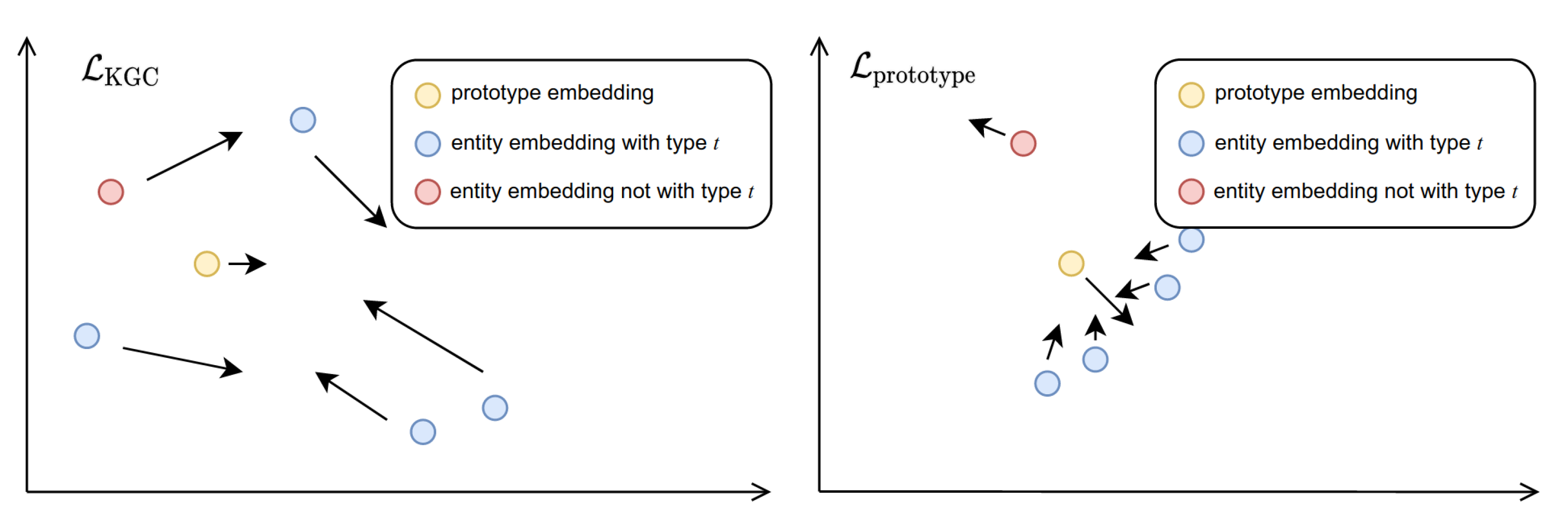
. The effects of loss functions on embeddings in the optimization are explained in Figure 3. The procedure of adjusting entity and prototype embeddings by L KGC and L prototype is shown on the left and right, respectively. The yellow point is the prototype embedding for type x. Blue points are entity embeddings whose type is represented by the prototype embedding. The red point is an entity embedding whose type should not be represented by the prototype embedding. Arrows represent the movement directions of embeddings by the gradients in the optimization. The figure on the left shows the accumulated adjustment from L KGC in T epochs. Due to the gradients from the sigmoid function in f ProtoE , the offset of prototype embeddings is not as significant as that for entity embeddings. The right figure shows the calibration of embeddings from gradients by L prototype at the T-th epoch. Because of the different learning rates for these two loss functions, offsets from L prototype are not as significant as those in the left figure, but the movement directions are more toward the location in which the prototype embeddings are located.

4. Experiments

We used three datasets to test our method, namely FB15k-237, WN18RR, and YAGO3-10. FB15k-237 and YAGO3-10 are, respectively, subsets of the knowledge graphs Freebase [33] and YAGO [34]. These two knowledge graphs store facts about the real world. WN18RR is a subset of WordNet [35]. Facts in WordNet describe relations between English words. The statistics of these three datasets are shown in Table 1.

4.1. Baselines and Hyperparameter Settings

For unsupervised implicit type representation learning, we chose the following methods as baselines.
1
TypeComplEx and TypeDistMult [25] are general methods for bilinear models to learn implicit type representations. They use independent feature spaces for representations of entity type and relation type constraints. A brief introduction is given in Section 2, Equation (6). We also applied the model to TransE (TypeTransE model).
2
AutoEter [23] is a method that integrates TransE [4], TransH [5], TransR [6], and RotatE [17] as one model to learn implicit type representations. The score function for capturing the interdependence of head and tail entities is based on RotatE, and the score function used to evaluate type compatibility is based on TransR.
For type-agnostic KGC models that serve as the base model in unsupervised learning for implicit type representations, we chose TransE [4], TransR [6], RotatE [17], DistMult [7], and ComplEx [9]. DistMult and ComplEx were used to evaluate the performance on bilinear models with a real or complex feature space, and TransE [4] and TransR [6] were used to test the performance on translational models with and without projection matrices. We enhanced RotatE [17] by ProtoE to compare the results to AutoEter [23]. The idea from TypeDistMult and TypeComplEx was also applied to TransE.
The hyperparameter settings for DistMult, ComplEx, and TypeDistMult and TypeComplEx follow those in a previous study [25]. We also applied the same method [25] to TransE by replacing f Base in Equation (6) with f TransE in Equation (4). Due to numerical issues, the method proposed by Jain et al. [25] could not be applied to TransR (the norm constraints in TransR result in float number underflow due to the sigmoid function on f Base in Equation (6)).
For TransR, we followed the instructions in the corresponding paper [6] but changed the embedding size to 100 for both entities and relations because we found that a large embedding size improves the performance of TransR. TransR and ProtoETransR were tested on FB15k-237 and WN18RR only because the number of entities in YAGO3-10 is much higher (about 3 times that for WN18RR and 8.5 times that for FB15k-237, cf. Table 1) than those in the other two datasets, and the project matrix in TransR consumes a lot of memory, resulting in difficult optimization (it takes about 33 h to train for 1000 epochs on YAGO3-10 for a single combination of hyperparameters with a single NVIDIA RTX Titan X GPU; it takes about 25 h with a NVIDIA A6000 GPU card). For the same reason, RotatE, AutoEter, and ProtoERotatE were not tested on YAGO3-10 due to the long training time of AutoEter.
All KGC models enhanced by ProtoE used the multiplication strategy in Equation (10) except for RotatE. ProtoERotatE used the addition strategy.
Because the negative sampling method for corrupted triples affects performance [17], we used a uniform distribution to sample the negative examples used in Equation (12) for a fair comparison. The number of negative examples was set to 20.
All parameters were randomly initialized by the Glorot uniform initializer [36]. The loss function used in training all models was the softmax loss in Equation (12) with θ = 20 . Other hyperparameters were optimized by grid search. We optimized all parameters using the Adam [37] optimizer. The hyperparameters and corresponding range of grid search are summarized as follows.
1
Max epoch: 1000;
2
Learning rate β KGC : { 0.005 , 0.001 , 0.0005 , 0.0001 , 0.00005 , 0.00001 } ;
3
Prototype loss learning rate β prototype : { 0.005 , 0.001 , 0.0005 , 0.0001 , 0.00005 , 0.00001 } ;
4
2 regularizer weight β : { 0.005 , 0.001 , 0.0005 , 0.0001 , 0.00005 , 0.00001 } ;
5
Batch size B: { 1024 , 2048 , 4096 , 8192 , 16348 } ;
6
Prototype number N r and M r : { 2 , 3 , 5 , 10 , 20 } ;
7
Prototype loss interval T: { 50 , 100 , 150 , 200 , 400 , 600 } ;
8
α in Equation (10) is −4.0 for translational models that evaluate implausibility and 4.0 for all other type-agnostic KGC models.
The dimension of the type representation feature space in AutoEter was set to 20 to make the size the same as that for TypeDistMult, TypeComplEx, and TypeDistMult. We used the mean reciprocal rank (MRR) as the criterion to choose the best hyperparameter combination. The NVIDIA A6000 GPU can handle the grid search of the hyperparameters (except for a few combinations for TransR).

4.2. Evaluation Metrics

We used two performance metrics, namely MRR and Hits@N, to evaluate performance. We corrupted facts ( h , r , t ) in the validation and test sets to the forms ( h , r , ? ) and ( ? , r , t ) . The corrupted triples were fed into the KGC models as a query, and all entities in the knowledge graph were ranked based on the score function. We removed all known correct answers h * and t * for which ( h * , r , t ) D train (for ( ? , r , t ) ) or ( h , r , t * ) D train (for ( h , r , ? )) before computing the rank. D train was the training set.
The MRR of an entity e is defined as follows.
MRR ( e ) = 1 rank ( e ) ,
where rank ( e ) is the rank of entity e. For a fact in the test or validation set ( h , r , t ) , let MRR head = rank ( h ) for ( ? , r , t ) and MRR tail = rank ( t ) for ( h , r , ? ) . The MRR of this record is computed as
MRR ( h , r , t ) = MRR head + MRR tail 2 .
The overall MRR is computed as
MRR = ( h , r , t ) D MRR ( h , r , t ) | D | ,
where D is the validation or test set. | D | is the cardinality of the set D . The overall MRR is in the range ( 0 , 1 ] .
For ( h , r , t ) D , if rank ( h ) N for the corrupted triple ( ? , r , t ) , Hits @ N head ( h , r , t ) = 1 . Similarly, if rank ( t ) N for ( h , r , ? ) , Hits @ N tail ( h , r , t ) = 1 . The overall Hits@N is computed as:
Hits @ N = 1 | D | ( h , r , t ) D Hits @ N head ( h , r , t ) + Hits @ N tail ( h , r , t ) 2 .
Similar to the overall MRR, the overall Hits @ N [ 0 , 1 ] .

4.3. Experimental Results and Discussion

The experimental results are shown in Table 2, Table 3 and Table 4. Our method improves all base KGC models in all performance metrics except for Hits@3, Hits@5, and Hits@10 for TransR, Hits@1 for DistMult on WN18RR, and Hits@1 for RotatE on FB15k-237.
As shown in Table 2, our method outperforms other methods in most metrics for FB15k-237. The improvement of KGC models with a feature space in the real domain is more significant than that with ComplEx, which uses a feature space in the complex domain. The reason is that ComplEx has twice the number of parameters as those of the other KGC models that use a feature space in R n . Therefore, prototype embeddings in ComplEx need more training data for each relation as the feature space is enlarged.
Table 3 shows that the performance improvement in link prediction applies to WN18RR even though it is difficult to define the type on entities in it. Facts in the WN18RR dataset describe relations between English words such as hypernym_of and hyponym_of. Hence, it is difficult to define the type and type constraints of entities in WN18RR. In this case, our method utilizes few prototype embeddings ( m = n = 2 for prototype matrices P r h and P r t in Equation (10)) to represent areas in which embeddings of suitable entities are located. Entities that have a high inner product with these prototype embeddings are more likely to be suitable for the corresponding relations. The prototype embeddings help to distinguish different entities in the feature space for translational models. In the original TransE and TransR, if ( h 1 , r , t ) and ( h 2 , r , t ) are two facts about r and t, the (projected) embeddings have the relation h 1 h 2 because of the score function. During optimization, the prototype embeddings associated with r have an effect on h 1 and h 2 , i.e., they increase the difference h 1 h 2 , improving the overall MRR of TransE and TransR. For DistMult, which is unable to model asymmetric relations (for example, the antonym_of relation in WN18RR), the modified score function in Equation (10) breaks the symmetry of f DistMult in Equation (2), improving performance.
As discussed in Section 3, the number of training examples of each relation affects the performance of our method. This is reflected by the results in Table 4. The number of training examples per relation in YAGO3-10 is larger than those for the other two datasets, and thus the improvement of the base models is larger for this dataset.
Moreover, as indicated in Table 2, Table 3 and Table 4, our method improves the performance of KGC models in different categories. DistMult and ComplEx are bilinear models. TransE and TransR are translational models. RotatE is similar to translational models but uses rotation instead of an offset vector to compute distance. All of these type-agnostic KGC models are improved by our approach.
In addition, we investigated the effect of the number of prototype embeddings in our method on the KGC model performance. Table 5, Table 6 and Table 7 show the results of ablation experiments for various numbers of prototype embeddings per relation (2, 3, 5, or 10). The number of prototype embeddings is shown in parenthesis. These results indicate that:
1
For FB15k-237 and YAGO3-10, it is better to have more prototype embeddings. If the number of prototype embeddings is insufficient to capture type constraints in all relations, the performance of the KGC model will degrade. Most type-agnostic KGC models enhanced by ProtoE need at least five prototype embeddings per relation. However, for WN18RR, the optimal number of prototype embeddings depends on the base KGC model because the type constraints in WN18RR are vague (e.g., hypernym_of, hyponym_of). In this case, our method relies on the capability of the base KGC model to capture the appropriate local areas in the feature space for relations.
2
The number of prototype embeddings depends on the properties of the knowledge graph and those of the base KGC model. For example, as shown for TransE with and without ProtoE on YAGO3-10 in Table 7, if the number of prototype embeddings is too small to represent type constraints, the type compatibility will degrade performance. In addition, different models need different numbers of prototype embeddings. From the results in Table 6, ProtoEDistMult and ProtoEComplEx need two prototype embeddings whereas ProtoETransE and ProtoERotatE need ten. The number of prototype embeddings depends on the properties of the knowledge graph (i.e., whether the relation type constraints are strict) and those of the base KGC models (whether they can capture triples using learned embeddings).
Furthermore, we evaluated the ability of our method to capture implicit entity types in FB15k-237. We matched entities in the FB15k-237 dataset to the same entities in Wikidata based on Freebase ID and took the label of objects in the instance_of relation from Wikidata as the entity type and the query entity types based on the entity ID in FB15k-237. The five highest frequency types, namely class of award, film, human, association football club, big city, music genre, television series, and city of the United States were used for clustering to test the ability of our model and the base KGC model to distinguish entity types. These five types are associated with 53.35% (7758/14,541) of the entities in FB15k-237. These entities are clustered by t-SNE [38] with embeddings from DistMult and ProtoEDistMult (with the number of prototypes set to 10 for the head and the tail) to explain the difference in entity embedding locations in both models. The clustering results in Figure 4 show that:
1
Both models can distinguish entities with types film, human, and television series. The boundaries of these three clusters are obvious. The clusters of entities with types big city and city of the United States overlap because these two types share many common entities.
2
The clusters of class of award, big city, and music genre slightly intersect with the entity embeddings from DistMult, and our method distinguishes music genre from the other types because the locations of the entity embeddings are calibrated using the prototype embeddings in relations.
As introduced in Section 3, the prototype embeddings also capture the local areas for entities that satisfy the type constraints in relation r. We visualize the entity and prototype embeddings in the relation /film/actor/film./film/performance/film (denoted as perform_in in the following text) in Figure 5 to explain the relationship of locations between entity and prototype embeddings in the feature space. The visualized entities are from the training set. In this relation, the head entity is an actor or actress and, the tail entity is a film in which they acted in. The head prototype embeddings and the tail prototype embeddings are denoted by black and yellow dots, respectively. The results in Figure 5 show that the prototype embeddings in the relation converge to nearly the same location in the feature space because all heads have the type “actor/actress” and all tails have the type “film”.
The number of training examples for a specific relation affects the convergence of the prototype embeddings associated with it. In the case where there are insufficient training examples and a limited number of entities in the relation, only some of the prototype embeddings converge to the desired locations. The others barely move from their initial location. The relation /user/jg/default_domain/olympic_games/sports (abbreviated as olympic_sports in the following text) is taken as an example to demonstrate this effect. There are 581 records in the training data for this relation (with 40 different head entities and 51 different tail entities), much fewer than those for the relation performed_in, which has 9696 records in the training data (with 2046 different head entities and 1784 different tail entities). In this relation, the head entities are the Olympic Games in different years and the tail entities are sports in these games. Figure 6 shows the clustering results of entity and prototype embeddings for this relation. The head prototypes and tail prototypes close to the center of the figure are redundant; their locations barely change from the initial locations due to the insufficient training examples and entities. However, this does not prevent the prototype embeddings in the left-top and right-bottom from capturing the local areas where the head entities and tail entities are located.
Additionally, we also examined the ability to capture multiple-type constraints in relations. Figure 7 shows the entity clustering results for ProtoEDistMult and TypeDistMult. Both models recognize the multiple entity types in the heads, but TypeDistMult cannot capture the type constraints entailed in these multiple clusters because it has only one type constraint embedding on the head. This relation has 273 different head entities, 7 different tail entities, and 335 records in the training data. ProtoE captures the four clusters using head prototype embeddings.
More clustering results for prototype embeddings and entity embeddings in relations can be found in Appendix A.

5. Conclusions

We proposed ProtoE as a general approach for extending translational and bilinear KGC models to have the ability to capture entity type and type constraints in relations. Different from supervised approaches, which require annotated type information, our method relies on only facts in the knowledge graph. Unlike previous unsupervised type inference methods, which can represent only a single type constraint in relations, our method can represent multiple type constraints in relations using prototype embeddings. Our method can be applied to both translational and bilinear KGC models. We associate prototype embeddings to represent type constraints on the subject and object of each relation. Prototype embeddings represent the local areas in which the embeddings of entities that satisfy the type constraint are located. To achieve this goal, the entity and relation embeddings in the base models and the prototype embeddings in our method are simultaneously trained using the facts in the knowledge graph. We use an optional extra loss function to calibrate the location of prototype embeddings to better represent diverse entity types in knowledge graphs.
The ability of prototype embeddings to capture entity type and type constraints in the relation r depends on the number of training data about r. For relations with sufficient training data and diverse entities, prototype embeddings well converge to the locations in which the density of qualified entity embeddings is high. In contrast, if the number of training data is insufficient, some prototype embeddings may not move from their initial location, but this does not affect the ability of the prototype embeddings to represent type constraints and entity types because some other prototype embeddings will be optimized to the high-density area where qualified entities are located. In the current setting, the number of prototype embeddings associated with relations is hyperparameters, and all relations have the same number of prototype embeddings for the head and the tail. This can be improved by combining the current method with stochastic processes, such as the Chinese restaurant process and the determinantal point process, to automatically set the number of prototype embeddings in relations. In the future, we plan to integrate these processes into our method to eliminate the need for setting the number of prototype embeddings as hyperparameters.
The experimental results for link prediction and entity clustering show that our method improves the performance of base KGC models in link prediction even though it is difficult to define the type of entities in the knowledge graph. In this case, prototype embeddings lose the identity of the type indicator and become representative embeddings for the local areas in which appropriate entity embeddings are located. The entity clustering results show that our method better captures the entity type and type constraints compared with other methods.

Author Contributions

Conceptualization—the concept behind this research was proposed by Y.L. and revised under suggestions from R.I.; formal analysis—the derivations were conducted by Y.L. and proofread by R.I.; funding acquisition—R.I.; investigation—the code was developed by Y.L.; methodology—the model was created by Y.L. and evolved under suggestions from R.I.; supervision—R.I.; validation and visualization—Y.L. and R.I.; writing—original draft: Y.L.; writing—review and editing: Y.L. and R.I. All authors have read and agreed to the published version of the manuscript.

Funding

This research was supported by the National Institute of Informatics and The Graduate University for Advanced Studies.

Institutional Review Board Statement

Not applicable.

Informed Consent Statement

Not applicable.

Data Availability Statement

All datasets are available at https://github.com/TimDettmers/ConvE accessed on 25 July 2022. Please contact lu-yuxun@nii.ac.jp and ichise@iee.e.titec.ac.jp for the code of ProtoE.

Conflicts of Interest

The authors declare no conflict of interest.

Appendix A. Additional Visualization of Clustering Results

Additional results for entity clustering are provided in this appendix. The text at the top of each figure is the name of the relation in the FB15k-237 dataset. The figure captions give the number of records in the training data concerning the relation and the numbers of different head and tail entities in the training data.
Figure A1. A total of 57 different head entities, 209 different tail entities, and 154 records in the training data.
Information 13 00354 g0a1
Figure A2. A total of 1,127 different head entities, 13 different tail entities, and 1151 records in the training data.
Information 13 00354 g0a2
Figure A3. A total of 235 different head entities, 116 different tail entities, and 251 records in the training data.
Information 13 00354 g0a3
Figure A4. A total of 93 different head entities, 90 different tail entities, and 99 records in the training data. Some of the head entities and tail entities overlap because the relation is symmetric.
Information 13 00354 g0a4

References

  1. Lu, Y.; Fang, Y.; Shi, C. Meta-learning on heterogeneous information networks for cold-start recommendation. In Proceedings of the 26th ACM SIGKDD International Conference on Knowledge Discovery & Data Mining, Virtual Event, CA, USA, 6–10 July 2020; pp. 1563–1573. [Google Scholar]
  2. Zhang, Y.; Dai, H.; Kozareva, Z.; Smola, A.J.; Song, L. Variational Reasoning for Question Answering with Knowledge Graph. In Proceedings of the 32nd AAAI Conference on Artificial Intelligence, New Orleans, LA, USA, 2–7 February 2018; pp. 6069–6076. [Google Scholar]
  3. Ji, G.; He, S.; Xu, L.; Liu, K.; Zhao, J. Knowledge Graph Embedding via Dynamic Mapping Matrix. In Proceedings of the 53rd Annual Meeting of the Association for Computational Linguistics, Beijing, China, 27–31 July 2015; pp. 687–696. [Google Scholar]
  4. Bordes, A.; Usunier, N.; Garcia-Duran, A.; Weston, J.; Yakhnenko, O. Translating Embeddings for Modeling Multi-relational Data. Adv. Neural Inf. Process. Syst. 2013, 26, 2787–2795. [Google Scholar]
  5. Wang, Z.; Zhang, J.; Feng, J.; Chen, Z. Knowledge Graph Embedding by Translating on Hyperplanes. In Proceedings of the 28th AAAI Conference on Artificial Intelligence, Quebec City, QC, Canada, 27–31 July 2014; pp. 1112–1119. [Google Scholar]
  6. Lin, Y.; Liu, Z.; Sun, M.; Liu, Y.; Zhu, X. Learning Entity and Relation Embeddings for Knowledge Graph Completion. In Proceedings of the 29th AAAI Conference on Artificial Intelligence, Austin, TX, USA, 25–30 January 2015; pp. 2181–2187. [Google Scholar]
  7. Yang, B.; Yih, W.T.; He, X.; Gao, J.; Deng, L. Embedding Entities and Relations for Learning and Inference in Knowledge Bases. In Proceedings of the International Conference on Learning Representations, San Diego, CA, USA, 7–9 May 2015. [Google Scholar]
  8. Nickel, M.; Tresp, V.; Kriegel, H.P. A Three-Way Model for Collective Learning on Multi-Relational Data. In Proceedings of the 28th International Conference on International Conference on Machine Learning, Madison, WI, USA, 28 June–2 July 2011; pp. 809–816. [Google Scholar]
  9. Trouillon, T.; Welbl, J.; Riedel, S.; Gaussier, E.; Bouchard, G. Complex Embeddings for Simple Link Prediction. In Proceedings of the 33rd International Conference on International Conference on Machine Learning, New York, NY, USA, 19–24 June 2016; pp. 2071–2080. [Google Scholar]
  10. Balazevic, I.; Allen, C.; Hospedales, T. TuckER: Tensor Factorization for Knowledge Graph Completion. In Proceedings of the 2019 Conference on Empirical Methods in Natural Language Processing, Hong Kong, China, 3–7 November 2019; pp. 5185–5194. [Google Scholar]
  11. Nickel, M.; Rosasco, L.; Poggio, T. Holographic Embeddings of Knowledge Graphs. In Proceedings of the 30th AAAI Conference on Artificial Intelligence, Phoenix, AZ, USA, 12–17 February 2016; pp. 1955–1961. [Google Scholar]
  12. Kazemi, S.M.; Poole, D. SimplE Embedding for Link Prediction in Knowledge Graphs. In Proceedings of the 32nd International Conference on Neural Information Processing Systems, Montreal, QC, Canada, 3–8 December 2018; pp. 4289–4300. [Google Scholar]
  13. Liu, H.; Wu, Y.; Yang, Y. Analogical Inference for Multi-Relational Embeddings. In Proceedings of the 34th International Conference on Machine Learning, Sydney, NSW, Australia, 6–11 August 2017; Volume 70, pp. 2168–2178. [Google Scholar]
  14. Dettmers, T.; Minervini, P.; Stenetorp, P.; Riedel, S. Convolutional 2D Knowledge Graph Embeddings. In Proceedings of the 32nd AAAI Conference on Artificial Intelligence, New Orleans, LA, USA, 2–7 February 2018; pp. 1811–1818. [Google Scholar]
  15. Ebisu, T.; Ichise, R. Generalized Translation-Based Embedding of Knowledge Graph. IEEE Trans. Knowl. Data Eng. 2020, 32, 941–951. [Google Scholar] [CrossRef]
  16. Li, Z.; Xu, Q.; Jiang, Y.; Cao, X.; Huang, Q. Quaternion-Based Knowledge Graph Network for Recommendation. In Proceedings of the 28th ACM International Conference on Multimedia, Seattle, WA, USA, 12–16 October 2020; pp. 880–888. [Google Scholar]
  17. Sun, Z.; Deng, Z.H.; Nie, J.Y.; Tang, J. RotatE: Knowledge Graph Embedding by Relational Rotation in Complex Space. In Proceedings of the International Conference on Learning Representations, New Orleans, LA, USA, 6–9 May 2019. [Google Scholar]
  18. Xie, R.; Liu, Z.; Sun, M. Representation Learning of Knowledge Graphs with Hierarchical Types. In Proceedings of the 25th International Joint Conference on Artificial Intelligence, New York, NY, USA, 9–15 July 2016; pp. 2965–2971. [Google Scholar]
  19. Zhao, Y.; Zhang, A.; Xie, R.; Liu, K.; Wang, X. Connecting Embeddings for Knowledge Graph Entity Typing. In Proceedings of the 58th Annual Meeting of the Association for Computational Linguistics, Seattle, WA, USA, 5–10 July 2020; pp. 6419–6428. [Google Scholar]
  20. Cui, Z.; Kapanipathi, P.; Talamadupula, K.; Gao, T.; Ji, Q. Type-augmented Relation Prediction in Knowledge Graphs. In Proceedings of the 35th AAAI Conference on Artificial Intelligence, Virtual, 2–9 February 2021. [Google Scholar]
  21. Moon, C.; Jones, P.; Samatova, N.F. Learning Entity Type Embeddings for Knowledge Graph Completion. In Proceedings of the 2017 ACM on Conference on Information and Knowledge Management, Singapore, Singapore, 6–10 November 2017; pp. 2215–2218. [Google Scholar]
  22. Krompaß, D.; Baier, S.; Tresp, V. Type-Constrained Representation Learning in Knowledge Graphs. In Proceedings of the 14th International Semantic Web Conference, Bethlehem, PA, USA, 13–15 October 2015; pp. 640–655. [Google Scholar]
  23. Niu, G.; Li, B.; Zhang, Y.; Pu, S.; Li, J. AutoETER: Automated Entity Type Representation for Knowledge Graph Embedding. Find. Assoc. Comput. Linguist. Emnlp 2020, 2020, 1172–1181. [Google Scholar]
  24. Ang, G.; Lim, E.P. Guided Attention Multimodal Multitask Financial Forecasting with Inter-Company Relationships and Global and Local News. In Proceedings of the 60th Annual Meeting of the Association for Computational Linguistics, Dublin, Ireland, 22–27 May 2022; pp. 6313–6326. [Google Scholar]
  25. Jain, P.; Kumar, P.; Chakrabarti, S. Type-sensitive knowledge base inference without explicit type supervision. In Proceedings of the 56th Annual Meeting of the Association for Computational Linguistics, Melbourne, Australia, 15–20 July 2018; pp. 75–80. [Google Scholar]
  26. Lu, Y.; Ichise, R. Unsupervised Type Constraint Inference in Bilinear Knowledge Graph Completion Models. In Proceedings of the 2021 IEEE International Conference on Big Knowledge, Auckland, New Zealand, 7–8 December 2021; pp. 15–22. [Google Scholar]
  27. Tucker, L.R. Some mathematical notes on three-mode factor analysis. Psychometrika 1966, 31, 279–311. [Google Scholar] [CrossRef] [PubMed]
  28. Hitchcock, F.L. The expression of a tensor or a polyadic as a sum of products. J. Math. Phys. 1927, 6, 164–189. [Google Scholar] [CrossRef]
  29. Mikolov, T.; Sutskever, I.; Chen, K.; Corrado, G.; Dean, J. Distributed Representations of Words and Phrases and Their Compositionality. In Proceedings of the 26th International Conference on Neural Information Processing Systems, Red Hook, NY, USA, 5–10 December 2013; pp. 3111–3119. [Google Scholar]
  30. Pennington, J.; Socher, R.; Manning, C.D. GloVe: Global Vectors for Word Representation. In Proceedings of the 2014 Empirical Methods in Natural Language Processing, Doha, Qatar, 25–29 October 2014; pp. 1532–1543. [Google Scholar]
  31. Che, F.; Zhang, D.; Tao, J.; Niu, M.; Zhao, B. ParamE: Regarding Neural Network Parameters as Relation Embeddings for Knowledge Graph Completion. In Proceedings of the AAAI Conference on Artificial Intelligence, Washington, DC, USA, 7–14 February 2020; pp. 2774–2781. [Google Scholar]
  32. Hayashi, K.; Shimbo, M. On the Equivalence of Holographic and Complex Embeddings for Link Prediction. In Proceedings of the 55th Annual Meeting of the Association for Computational Linguistics, Vancouver, Canada, 30 July–4 August 2017; pp. 554–559. [Google Scholar]
  33. Bollacker, K.; Evans, C.; Paritosh, P.; Sturge, T.; Taylor, J. Freebase: A Collaboratively Created Graph Database for Structuring Human Knowledge. In Proceedings of the 2008 ACM SIGMOD International Conference on Management of Data, New York, NY, USA, 9–12 June 2008; pp. 1247–1250. [Google Scholar]
  34. Suchanek, F.M.; Kasneci, G.; Weikum, G. Yago: A Core of Semantic Knowledge. In Proceedings of the 16th International Conference on World Wide Web, New York, NY, USA, 8–12 May 2007; pp. 697–706. [Google Scholar]
  35. Miller, G.A. WordNet: A Lexical Database for English. ACM Commun. 1995, 38, 39–41. [Google Scholar] [CrossRef]
  36. Glorot, X.; Bengio, Y. Understanding the difficulty of training deep feedforward neural networks. In Proceedings of the 13th International Conference on Artificial Intelligence and Statistics, Sardinia, Italy, 13–15 May 2010; pp. 249–256. [Google Scholar]
  37. Kingma, D.P.; Ba, J. Adam: A Method for Stochastic Optimization. In Proceedings of the International Conference on Learning Representations, San Diego, CA, USA, 7–9 May 2015. [Google Scholar]
  38. Van der Maaten, L.; Hinton, G. Visualizing data using t-SNE. J. Mach. Learn. Res. 2008, 9, 2579–2605. [Google Scholar]
Figure 1. Structure of TypeDM [25]. Entity embeddings and type embeddings are in different feature spaces (indicated by their colors).
Information 13 00354 g001
Figure 2. Structure of proposed method ProtoE. Each relation is associated with head prototypes and tail prototypes.
Information 13 00354 g002
Figure 3. Example of effects of L KGC and L prototype on adjustment of embedding locations.
Information 13 00354 g003
Figure 4. Clustering results of entity embeddings for ProtoEDistMult and DistMult. (a) ProtoEDistMult; (b) DistMult.
Information 13 00354 g004
Figure 5. Entity and prototype embeddings related to performed_in in the dataset FB15k-237.
Information 13 00354 g005
Figure 6. Visualization of prototype and entity embeddings in olympic_sports in FB15k-237.
Information 13 00354 g006
Figure 7. Clustering results for TypeDistMult and ProtoEDistMult. (a) ProtoEDistMult; (b) TypeDistMult.
Information 13 00354 g007
Table 1. Statistical information of datasets in our experiments.
NameEntityRelationTrainValidTest
FB15k-23714,541237272,11517,53520,466
WN18RR40,9431186,83530343134
YAGO3-10123,182371,079,04050005000
Table 2. Experimental results for FB15k-237. Best values are indicated in bold.
FB15k-237
MRRHits@1Hits@3Hits@5Hits@10
DistMult0.25020.16460.27550.33730.4279
TypeDistMult0.24730.16470.26950.33050.4168
ProtoEDistMult0.25350.16680.27990.34260.4301
blackblack ComplEx0.25090.16430.27620.33940.4288
TypeComplEx0.24310.16120.26550.32330.4129
ProtoEComplEx0.25140.16470.27670.34080.4290
blackblack TransE0.24820.16440.27490.33240.4190
TypeTransE0.26600.17550.29230.35730.4540
ProtoETransE0.26090.17780.28580.34500.4540
blackblack TransR0.19010.11440.20720.26060.3459
ProtoETransR0.19840.12510.21310.26670.3515
blackblack RotatE0.26470.18100.28860.34820.4383
AutoEter0.24760.17520.26920.32160.3953
ProtoERotatE0.26600.18040.28970.35390.4430
Table 3. Experimental results for WN18RR. Best values are indicated in bold.
WN18RR
MRRHits@1Hits@3Hits@5Hits@10
DistMult0.41660.37870.43790.45640.4817
TypeDistMult0.40520.37670.42360.43640.4513
ProtoEDistMult0.41730.37650.44030.46230.4872
blackblack ComplEx0.41330.37480.43430.45370.4767
TypeComplEx0.39420.35880.41850.43250.4486
ProtoEComplEx0.41710.37810.43840.45690.4817
blackblack TransE0.16390.00380.28460.37440.4419
TypeTransE0.22420.06650.35450.43030.4861
ProtoETransE0.18060.01600.31380.39420.4580
blackblack TransR0.15350.00990.27870.33890.3725
ProtoETransR0.21630.15330.25240.29320.3385
blackblack RotatE0.42140.38270.43990.46060.4901
AutoEter0.42160.38430.44020.45960.4901
ProtoERotatE0.42320.38660.44020.46060.4919
Table 4. Experimental results for YAGO3-10. Best values are indicated in bold.
YAGO3-10
MRRHits@1Hits@3Hits@5Hits@10
DistMult0.40690.30700.45950.52480.5996
TypeDistMult0.45910.35400.52330.58130.6504
ProtoEDistMult0.42920.33380.47890.54290.6141
blackblack ComplEx0.3960.29730.44710.44710.5918
TypeComplEx0.45210.35230.50720.56970.6443
ProtoEComplEx0.42600.32750.48190.54440.6201
blackblack TransE0.38210.27360.43780.50530.5985
TypeTransE0.23840.15150.26170.33010.4176
ProtoETransE0.40700.29640.46340.53820.6291
Table 5. Results of ablation experiments for prototype embedding on FB15k-237. Best values are indicated in bold.
FB15k-237
MRRHits@1Hits@3Hits@5Hits@10
DistMult0.25020.16460.27550.33730.4279
ProtoEDistMult (2)0.24910.16430.27420.33840.4275
ProtoEDistMult (3)0.25020.16410.27440.33640.4295
ProtoEDistMult (5)0.25030.16510.27440.33630.4270
ProtoEDistMult (10)0.25350.16680.27990.34260.4301
ComplEx0.25090.16430.27620.33940.4288
ProtoEComplEx (2)0.25120.16480.27700.33940.4297
ProtoEComplEx (3)0.24880.16390.27320.36630.4249
ProtoEComplEx (5)0.24970.16450.27530.33540.4240
ProtoEComplEx (10)0.25140.16470.27670.34080.4290
TransE0.24820.16440.27490.33240.4190
ProtoETransE (2)0.18740.12760.20220.24370.3080
ProtoETransE (3)0.18790.12940.20090.25220.3249
ProtoETransE (5)0.23510.15430.25840.31580.3978
ProtoETransE (10)0.26090.17780.28580.34500.4540
RotatE0.26470.18100.28860.34820.4383
ProtoERotatE (2)0.26070.17720.28390.34590.4353
ProtoERotatE (3)0.25910.17550.28310.34460.4322
ProtoERotatE (5)0.25330.16940.27770.33850.4265
ProtoERotatE (10)0.26600.18040.28970.35390.4430
Table 6. Results of ablation experiments for prototype embedding on WN18RR. Best values are indicated in bold.
WN18RR
MRRHits@1Hits@3Hits@5Hits@10
DistMult0.41660.37870.43790.45640.4817
ProtoEDistMult (2)0.41730.37650.44030.46230.4872
ProtoEDistMult (3)0.40860.37570.42710.44540.4655
ProtoEDistMult (5)0.40380.36930.42490.44050.4561
ProtoEDistMult (10)0.40750.37000.43040.44430.4671
ComplEx0.41330.37480.43430.45370.4767
ProtoEComplEx (2)0.41710.37810.43840.45690.4817
ProtoEComplEx (3)0.41060.37460.43190.44670.4690
ProtoEComplEx (5)0.40990.37510.43140.44610.4652
ProtoEComplEx (10)0.40930.37250.42960.44860.4703
TransE0.16390.00380.28460.37440.4419
ProtoETransE (2)0.02340.01340.02470.02990.0415
ProtoETransE (3)0.03050.00060.03300.04770.0766
ProtoETransE (5)0.09500.00090.14710.20390.2551
ProtoETransE (10)0.18060.01600.31380.39420.4580
RotatE0.42140.38270.43990.46060.4901
ProtoERotatE (2)0.42000.38290.43520.45740.4887
ProtoERotatE (3)0.42260.38480.43890.45820.4928
ProtoERotatE (5)0.42220.38340.44050.46140.4938
ProtoERotatE (10)0.42320.38660.44020.46060.4919
Table 7. Results of ablation experiments for prototype embedding on YAGO3-10. Best values are indicated in bold.
YAGO3-10
MRRHits@1Hits@3Hits@5Hits@10
DistMult0.40690.30700.45950.52480.5996
ProtoEDistMult (2)0.40250.30410.45270.51990.5969
ProtoEDistMult (3)0.42460.32380.49690.56040.6360
ProtoEDistMult (5)0.41750.32200.46820.52770.6046
ProtoEDistMult (10)0.42920.33380.47890.54290.6141
ComplEx0.39600.29730.44710.44710.5918
ProtoEComplEx (2)0.38790.28800.43780.50450.5836
ProtoEComplEx (3)0.38740.28960.43570.50010.5816
ProtoEComplEx (5)0.36920.27070.41750.48270.5657
ProtoEComplEx (10)0.42600.32750.48190.54440.6201
TransE0.38210.27360.43780.50530.5985
ProtoETransE (2)0.04330.03590.04250.04520.0433
ProtoETransE (3)0.04300.03590.04200.04620.0527
ProtoETransE (5)0.10160.04520.11760.14880.1966
ProtoETransE (10)0.40700.29640.46340.53820.6291
Publisher’s Note: MDPI stays neutral with regard to jurisdictional claims in published maps and institutional affiliations.

