
Supervised Learning Models for the Preliminary Detection of COVID-19 in Patients Using Demographic and Epidemiological Parameters

 , , , and
Abstract
:1. Introduction
- Extensive review of background research: We perform a detailed review of recent work in the literature, which looks at various diagnostic procedures for COVID-19 using AI and ML. Emphasis is placed on articles which consider demographic and epidemiological parameters as part of their data.
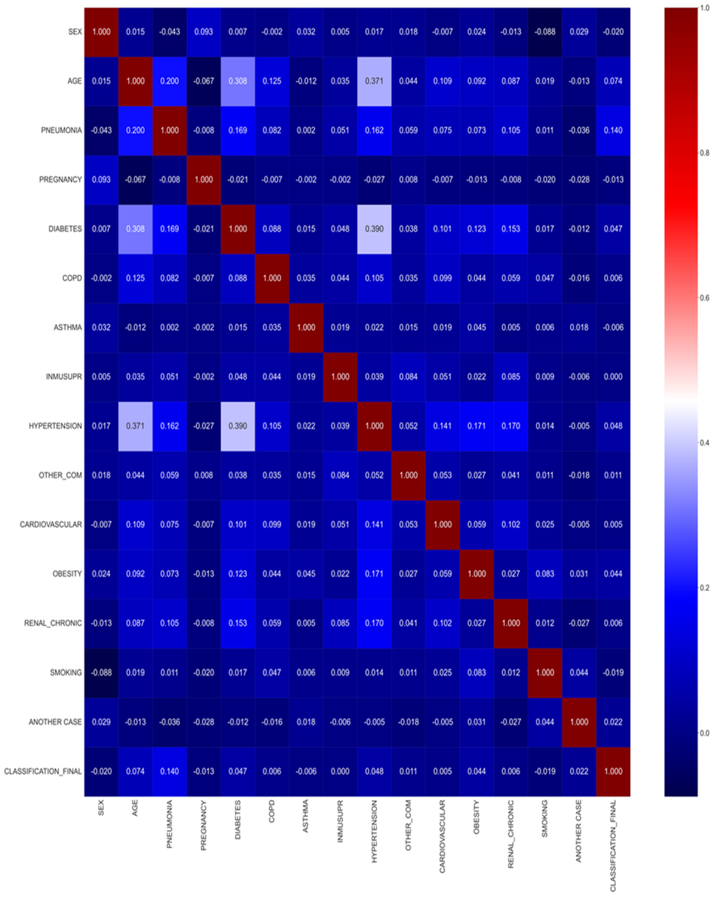
- Pre-processing: The data are pre-processed to understand the most important parameters. Correlation techniques have been used to underline the most important columns in the dataset.
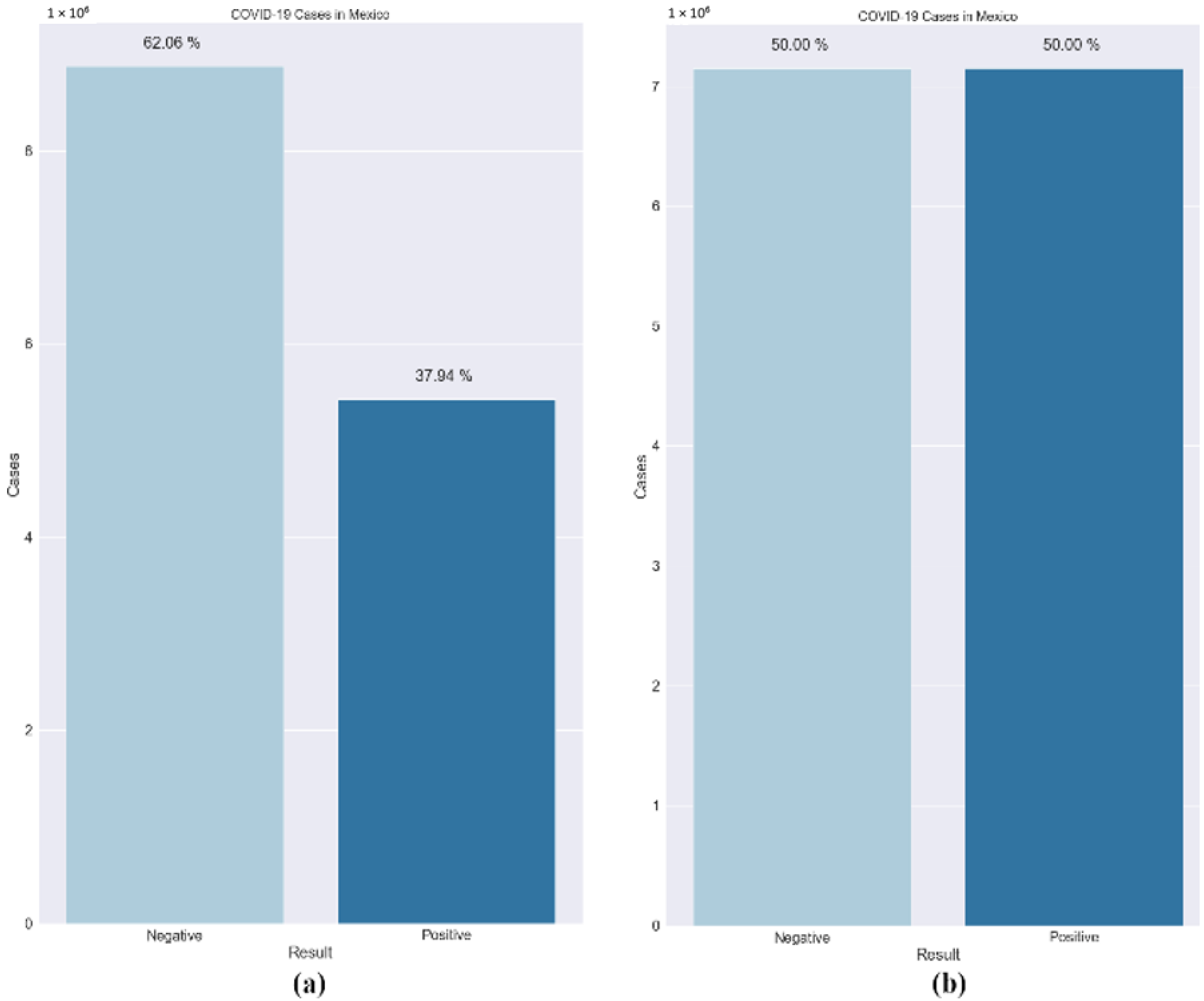
- Balancing: We use the Borderline-SMOTE technique to balance the data.
- Feature importance: We highlight relevant feature importance derivation techniques.
- Application of ML models: Machine learning and deep learning techniques have been used to derive insights from the data. As demonstrated below, the models tend to perform quite well for the considered data.
- Analysis of parameters: Information about the various parameters is obtained, and their effect on COVID-19 patients is studied. The results obtained are compared with state-of-the-art studies in the literature using similar data.
- Future directions: We provide an overview of some challenges faced and potential future directions to extend the work.
Motivation and Contributions
2. Related Work
3. Materials and Methods
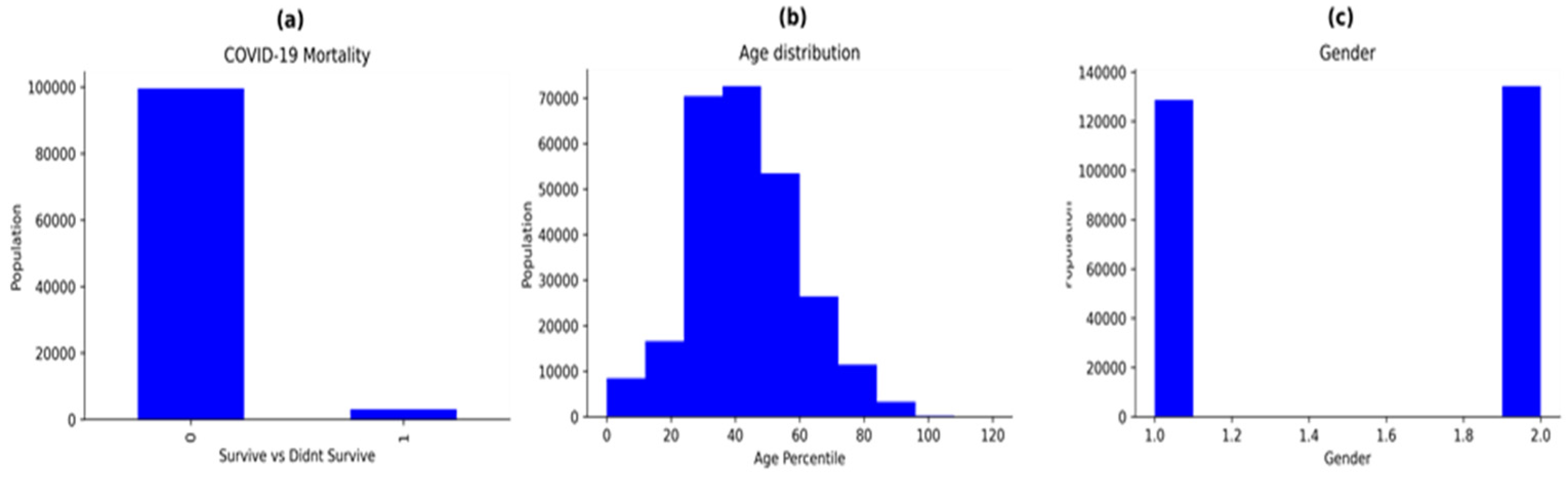
3.1. Dataset Description
3.2. Data Pre-Processing
3.3. Some Machine Learning Algorithms and Related Terminologies
- Logistic regression: For binary and multiclass classification problems, logistic regression is an extensively used statistical classification approach. The logistic function is used to forecast the likelihood of a class label [70]. The model gives exceptional results when the labels are binary. Contrary to its name, this is a classification model, not a regression model. It is quite simple to implement and achieves excellent performance when using linearly separable classes. It uses the sigmoid function to classify the instances. The mathematical equation for logistic regression can be given as:where P is the probability that Y belongs to class C and β0 and β1 are model parameters.
- Random forest: The random forest (RF) method is a widely used machine learning technique that interpolates the output of numerous decision trees (DT) to produce a single result [71]. It is based on the notion of ensemble learning, which is a method for integrating several weak classifiers in order to solve a complex problem. It can be used for both regression and classification problems. RF is a technique that extends the bagging approach by combining bagging with feature randomization to generate an uncorrelated forest of decision trees. It partitions the data into training and testing sets using the bootstrapping data sampling approach. The model builds trees repeatedly with each bootstrap. The final forecast is based on the average vote for each class. The larger the number of trees in the forest, the better the reliability. The chance of overfitting also decreases drastically. Further, it provides great flexibility since it can accurately perform classification and regression jobs with high accuracy. It can also be used to understand the importance of each feature. However, its main disadvantage is that these models are very complex and require much time and memory to train the models. The equations to calculate the Gini impurity and entropy are described in Equations (4) and (5). Both Gini impurity and entropy are measures of impurity of a node.where f is the frequency of the label and c represents the number of labels.
- XGBoost: The extreme gradient boosting (XGBoost) [72] algorithm is another prediction modelling algorithm based on ensemble learning, which can be applied to classification, regression and ranking problems. Generally, gradient boosting algorithms may suffer from overfitting as a result of data inequality [72]. However, the regularisation parameter in the XGBoost technique mitigates the danger of model overfitting. It is also an iterative tree-based ensemble classifier which seeks to improve the model’s accuracy by using a boosting data resampling strategy to decrease the classification error. The algorithm is composed of a number of parameters. The ideal parameter combination improves the model’s performance. It also makes use of the previous unsuccessful iteration results in the subsequent steps to achieve an optimal result. The XGBoost algorithm makes use of several CPU cores, allowing for simultaneous learning during training. The objective function of XGBoost is given by the sum of loss and regularization function as described in Equation (6).where fj is the prediction and where j is the tree (regularisation function).
- AdaBoost: Adaptive boosting, also referred to as AdaBoost, is a machine learning approach that uses the ensemble methodology [73]. It is a meta-algorithm for statistical classification that may be used in combination with a variety of learning algorithms to enhance performance [73]. It is a widely used algorithm and it makes use of the terminology named decision stumps, which are single-level decision trees (decision trees with just one split). A key feature of AdaBoost is its adaptivity based on the results of the previous classifiers. The first step of the algorithm involves constructing a model where all data points are assigned equal weights. Points that have been misclassified are provided with larger weights. With this change, the models deployed subsequently are expected to be more reliable. The model continues to train till it reduces its loss function. However, AdaBoost’s performance degrades when irrelevant features are added. It is also slow compared to XGBoost since it is not tuned for speed. The model function for AdaBoost is described in Equation (7).
- KNN: The k-nearest neighbours algorithm (k-NN or KNN) is a simple non-parametric supervised ML algorithm used for both regression and classification [74]. A dataset’s k closest training instances serve as the input for the model’s learning process. It is also known as a “lazy learner” algorithm since it does not utilise the input during training. The KNN algorithm is based on the principle of majority voting. It gathers information from the training dataset and utilises it to make predictions about subsequent records. The first step in a KNN algorithm is to select k number of neighbours where k is an optimal constant. Calculation of the Euclidean distance (or Hamming distance for text classification) is conducted to find the nearest data points. Choosing a suitable value of k is crucial as it affects the functioning of the algorithm. The benefits of the KNN model include its robustness, ease of implementation and its ability to pre-process large datasets. However, selecting the right k value requires expertise. Further, it also increases the computational time during testing.
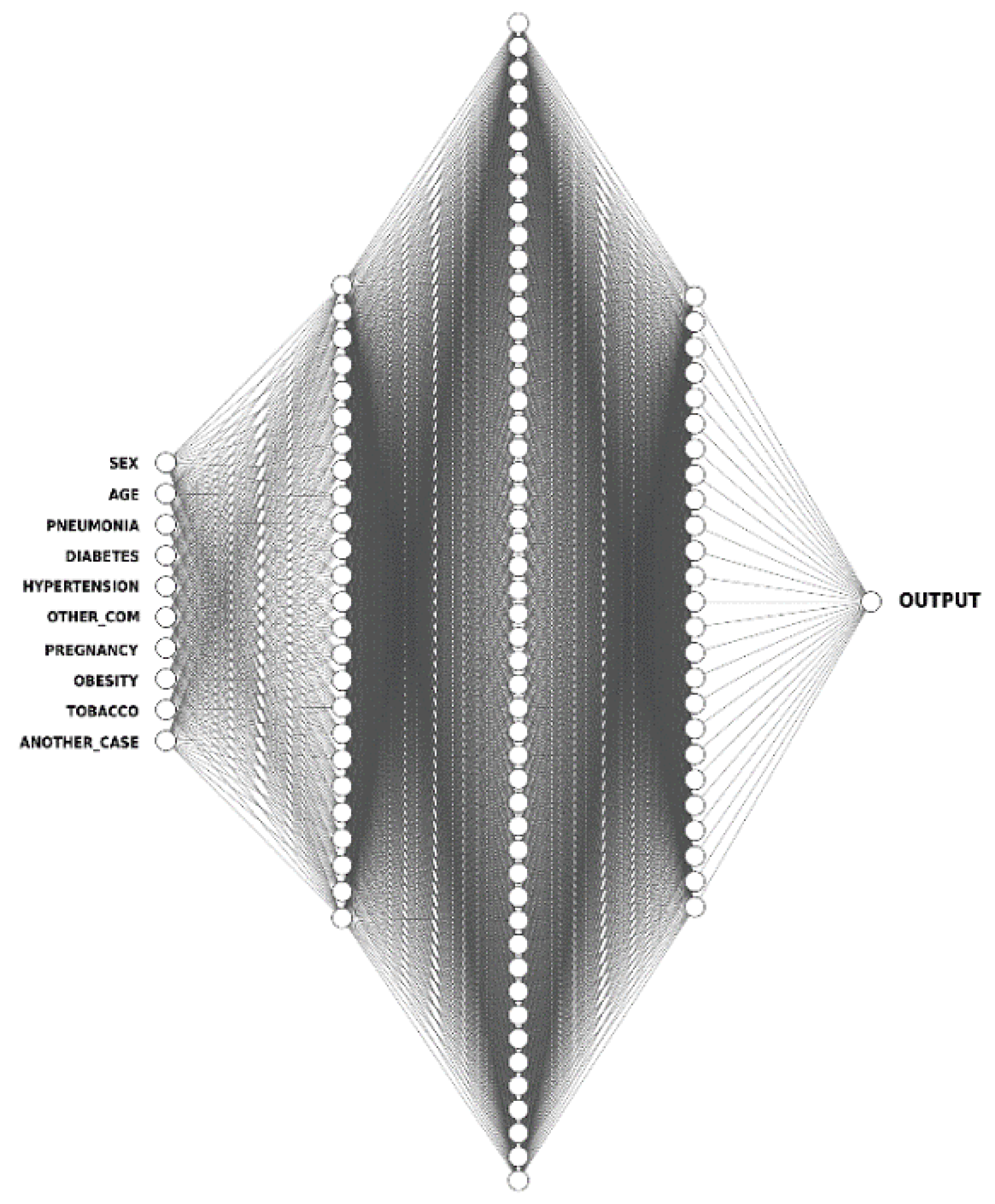
- ANN: Artificial neural networks (ANNs) mirror the human brain’s functioning, enabling software programs to discover patterns in large datasets [75]. They make use of nodes referred to as artificial neurons, interconnected over multiple layers of varying sizes to mimic the activities and roles of biological neural networks in the human brain. To their credit, ANNs have the ability to draw inferences about the correlations between variables which is not possible with other types of statistical models. The ANN architecture is composed of a series of node layers, they consist of a single input layer, connected to one or more hidden layers, which are then connected to an output layer. The nodes link to one another and each of them has a weight and threshold associated with it. Only when a node’s output exceeds a certain threshold, is it activated and begins transferring data to the network’s next layer. The node architecture for the ANN model is described in Figure 4.
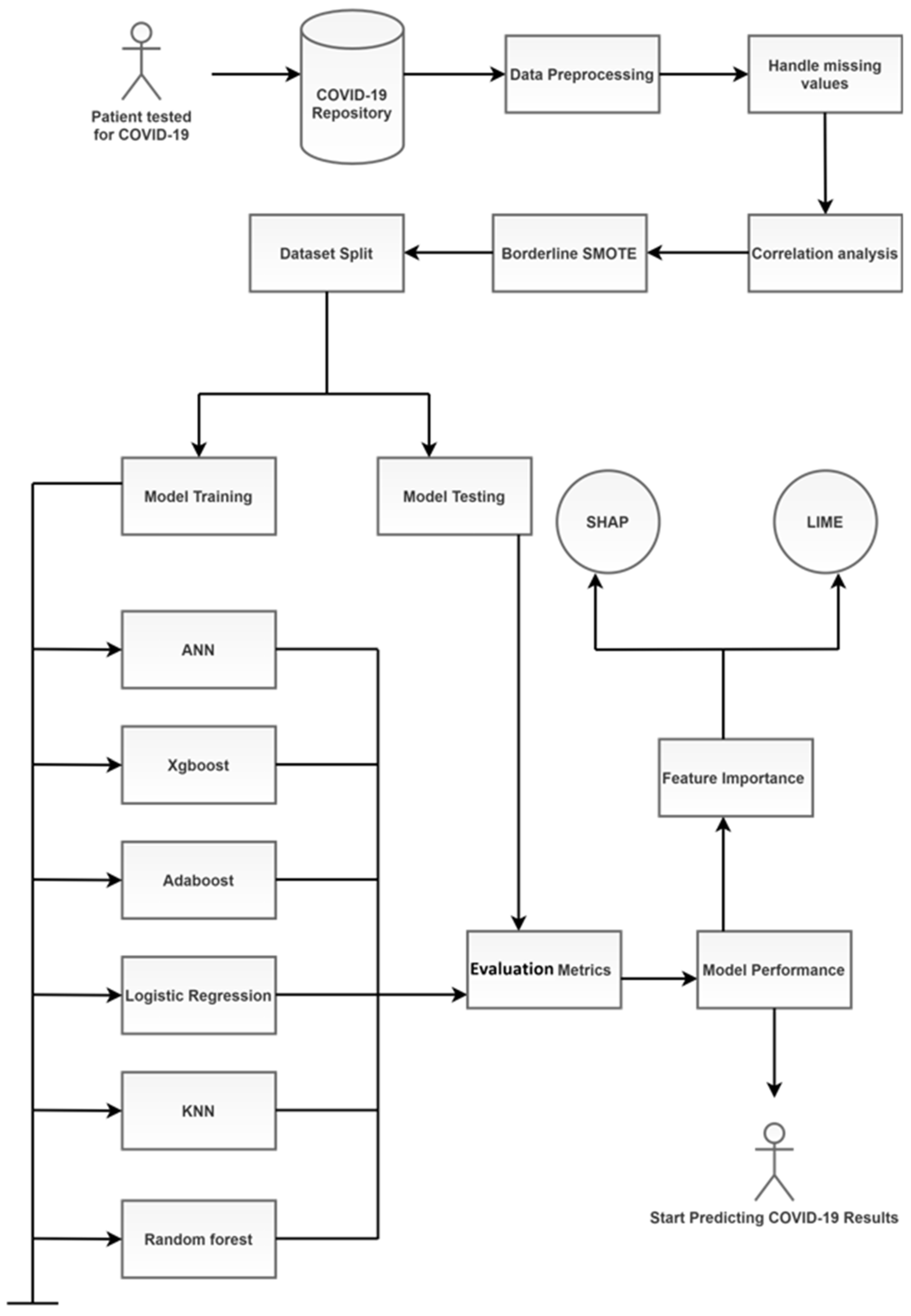
- SMOTE: Data imbalance is a common problem in medical machine learning and often results in overfitting. Imbalanced class distribution has a considerable performance penalty in comparison to most traditional classifier learning techniques that assume a generally balanced class distribution and equal misclassification costs. An effective method to overcome dataset imbalance in ML is by using the synthetic minority oversampling technique (SMOTE) [76]. SMOTE employs an oversampling technique to adjust the initial training set. Rather than just replicating minority class cases, SMOTE’s central concept is to offer new artificial instances which are similar to the minority class. This new dataset is constructed by interpolating between numerous occurrences of a minority class within a specific neighbourhood. In this research, a technique called the Borderline-SMOTE was used. It is based on the principle that borderline cases may provide negligible contribution to the overall success of the classification [77]. The models are more reliable when the data are balanced. Figure 5 shows the dataset before and after the use of the Borderline-SMOTE algorithm. Further, the training data were split randomly into an 80:20 ratio, with the larger proportion of the partition reserved for training the model. The smaller set was used for testing the models’ performance. It was made sure that both the subsets maintained a similar composition and lacked bias.
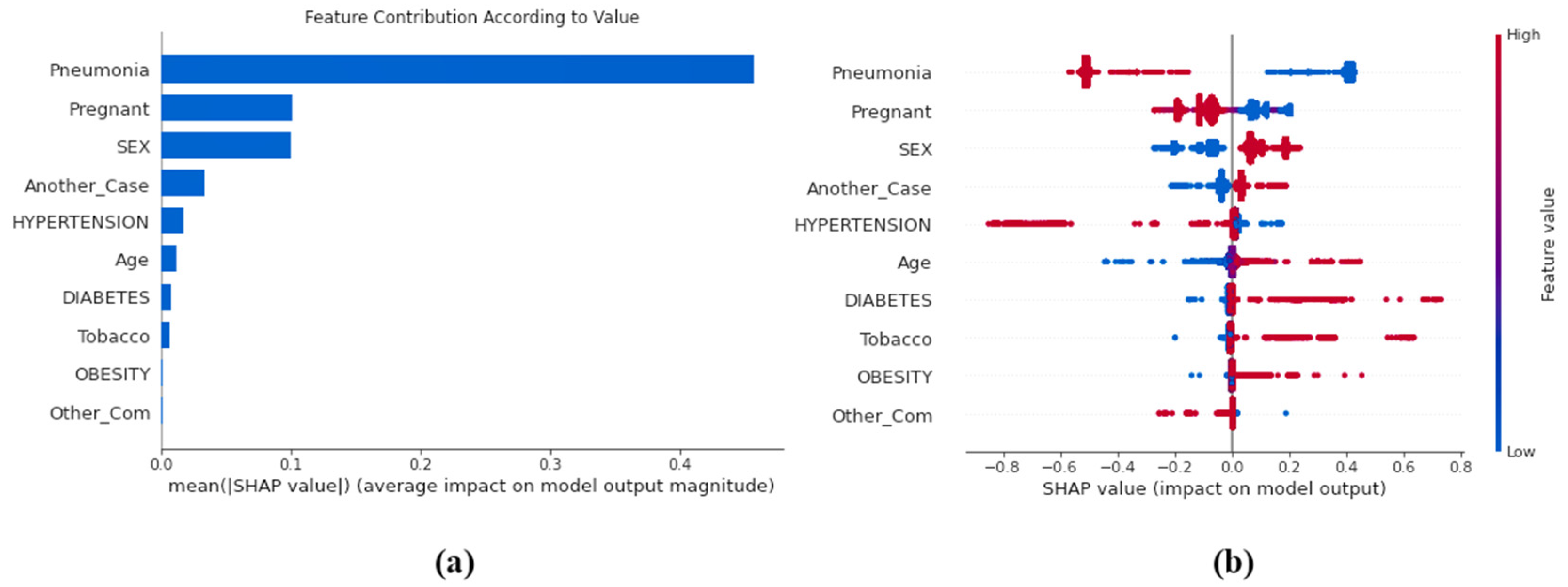
- Shapley Additive Values (SHAP): SHAP is based on the principle of game theory and it is used to increase the interpretability and transparency of the ML models [78]. Most ML and deep learning models are compatible with SHAP. The ‘Tree-Explainer’ procedure is mainly used in tree-based classifiers such as decision tree, random forest and other boosting algorithms. SHAP employs a variety of visual descriptions to convey the importance of attributes and how they influence the model’s decision making. The baseline estimates of various parameters are compared to forecast the prediction.
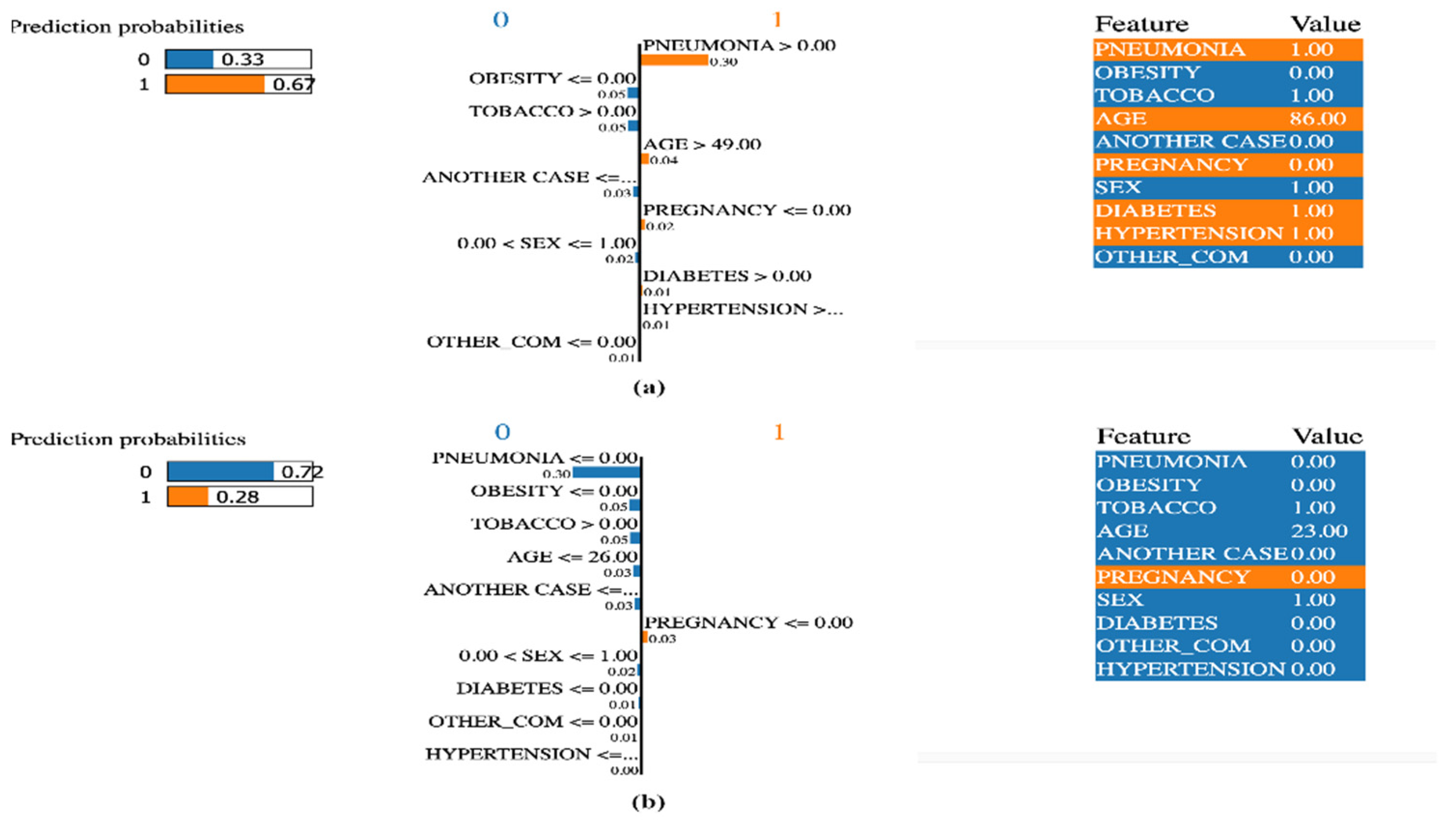
- Local Interpretable Model-Agnostic Explanations (LIME): LIME is independent of any model and can be used with all the existing classifiers [79]. By adjusting the source of data points and seeing how the predictions vary, the technique seeks to understand the model’s prediction. To acquire a deeper understanding of the black-box model, specific approaches look at the fundamental components and how they interact in LIME. It also modifies the attribute values in a particular order before assessing the impact on the whole outcome.
4. Results and Discussion
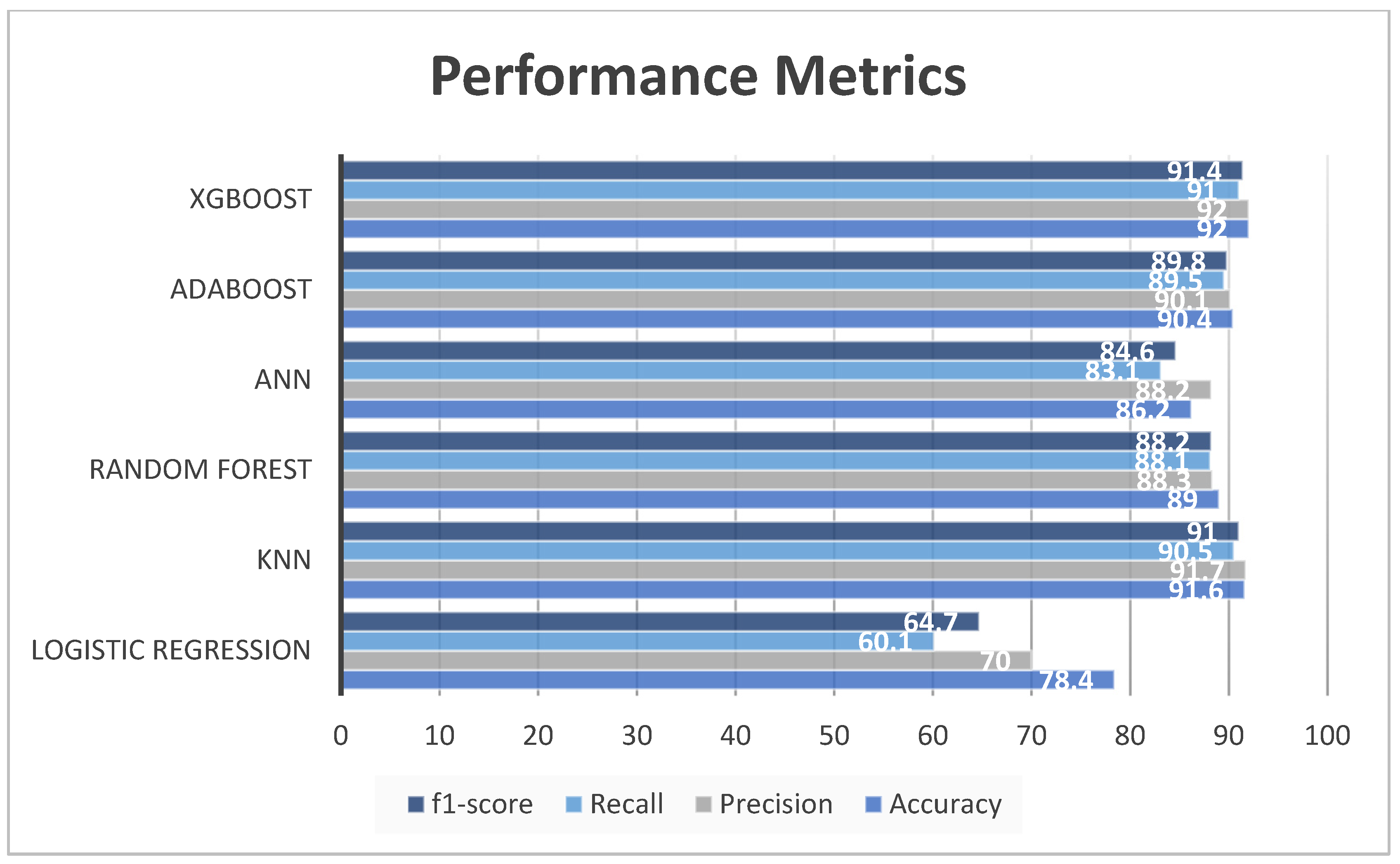
4.1. Performance Metrics
- Accuracy: It is a measurement which calculates the number of COVID-19 cases diagnosed accurately from the total number of cases. Correct diagnosis in this scenario is when the prediction for the case is positive, and its result is positive or when the prediction for the case is negative, and the result is also negative. It is an important metric to understand if the model is accurately diagnosing the virus. It is given by the formula:
- Precision: It is another metric which calculates the ratio of patients correctly diagnosed as COVID-19 positive from the total patients predicted as COVID-19 positive by the ML models. This means that it also considers the false-positive cases, which are the patients incorrectly diagnosed with COVID-19 positive diagnosis. This metric indicates the merit of the positive cases diagnosed by the algorithm and to understand that if a patient was predicted as COVID-19 positive by the model, what would be the likelihood of them being affected by it. It is given by the formula below:
- Recall: It is a performance metric that can be defined as the ratio of the patients correctly diagnosed as COVID-19 positive to the total patients infected by the virus. This metric emphasizes the false-negative cases. The recall is exceptionally high when the number of false-negative cases is low. It is calculated by the formula given below:
- F1-score: It is an estimate which gives equal importance to the precision and recall values obtained previously for the COVID-19 cases. It gives a better idea about the positive cases of the virus obtained. It is given by the following formula:
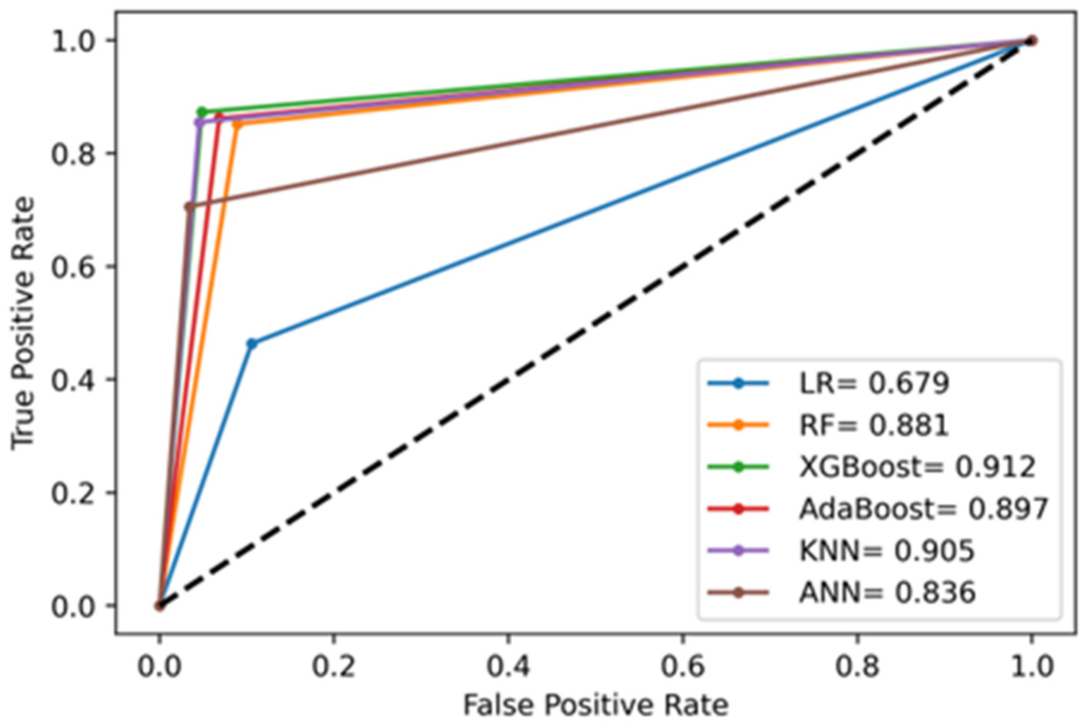
- AUC (area under curve): The ROC (receiver operating characteristic) curve plots the true positive rate against the false-positive rate for various test instances. It indicates how well the models are differentiating the binary classes. The area under this curve is the AUC. High values for AUC indicate that the classifier is performing well.
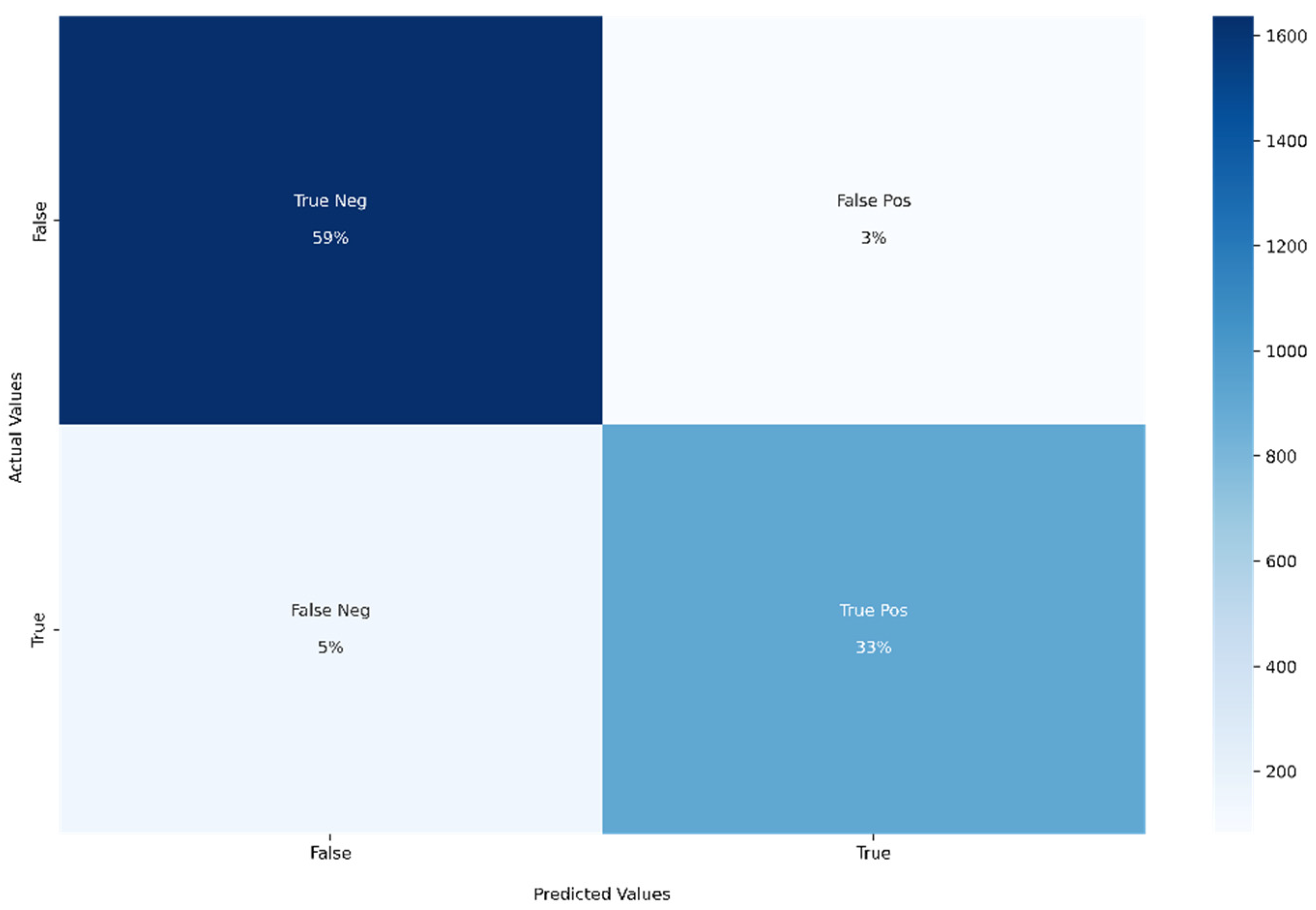
- Confusion matrix: For binary classification, the confusion matrix is a 2 × 2 matrix. All the classified instances will be in the confusion matrix. The diagonal elements indicate the correct classified instances (both true-positive and true-negative). The non-diagonal elements indicate the wrongly classified instances (both false-positive and false-negative). All the mentioned performance metrics can be easily calculated using the confusion matrix.
4.2. Model Evaluation
4.3. Feature Importance using SHAP and LIME
4.4. Further Discussion
5. Challenges and Future Directions
5.1. Challenges
- Data from a single country: For this research, data were collected from Mexico. However, data from all geographic areas must be considered for better validation. This is not a trivial task as there are clear differences in reporting standards and authenticity across different countries.
- Imbalance in data: In much of medical AI research, data imbalance is a persistent issue. The number of healthy patients is always more than the number of infected people. However, the models perform well when there are an equal number of classes. In this research, the Borderline-SMOTE technique was used to balance the data. Appropriate pre-processing should precede model training when working with such data.
- Original values: The data obtained for this research was already normalized. However, original data are required to form accurate medical intuitions.
- Missing blood and clinical markers: Clinical markers, such as CRP (C reactive protein), D-dimer, ferritin and lactate dehydrogenase (LDH) are known to be extremely useful in diagnosing COVID-19. However, these markers were not available in the dataset.
- Variance in computer equipment: There is no one single uniform standard architecture followed by machines universally. The data are quite sensitive to software and hardware changes of the setup.
- Distributional shift in test data: An ML model will struggle to perform well if it is unable to adapt to novel scenarios. Trained models in supervised learning are notoriously bad at detecting meaningful changes in context or data, which leads to inaccurate predictions based on out-of-scope data. When the ML method is incorrectly applied to an unexpected patient situation, it might cause a disparity between the learning and operational data.
- Difficulties in deploying AI systems on a logistical level: Numerous existing difficulties in converting AI applications to clinical practice are due to the fact that the majority of healthcare data are not easily accessible for machine learning. Data are often compartmentalised in a plethora of medical imaging archiving systems, electronic health records (EHR), pathology systems, electronic prescription tools and insurance databases, making integration very challenging.
- Interpreting the result: The model may be able to derive complex and hidden patterns. However, sometimes these patterns might have no meaning. This might be problematic in medical applications, where there is a high need for techniques that are not just effective, but also clear, interpretable and explainable.
- Quality of data: It is essential to obtain reliable input from authentic sources. It is also necessary to filter out the noise which may have crept in while feeding the data.
- Data privacy: Most of the medical data obtained from the patients are highly confidential. A leak, attack or misuse of it can be catastrophic.
5.2. Future Directions
- Improving the dataset: For further research, a more balanced dataset can be collected. Important clinical markers mentioned in the previous section can also be considered. COVID-19 severity can also be predicted.
- Using different algorithms: This research can be expanded by experimenting with different ML algorithms and combining them, as each model has its own pros and cons, there could be a model which is tailor-made for this dataset
- Medical validation: Medical validation can be performed by doctors to comment on the authenticity of the models. Further, the models can be deployed in medical facilities and feedback on accuracy can be incorporated.
- Combining other AI methodologies: CT-scans, X-rays, MRIs, ultrasound and cough sound analysis also use AI to diagnose COVID-19. The integration of these models is expected to produce compelling results.
6. Conclusions
Author Contributions
Funding
Institutional Review Board Statement
Informed Consent Statement
Data Availability Statement
Conflicts of Interest
References
- Woo, P.C.; Huang, Y.; Lau, S.K.; Yuen, K.Y. Coronavirus genomics and bioinformatics analysis. Viruses 2010, 2, 1804–1820. [Google Scholar] [CrossRef] [PubMed] [Green Version]
- Hayden, F.; Richman, D.; Whitley, R. Clinical Virology, 4th ed.; ASM Press: Washington, DC, USA, 2017. [Google Scholar]
- Huang, C.; Wang, Y.; Li, X.; Ren, L.; Zhao, J.; Hu, Y.; Zhang, L.; Fan, G.; Xu, J.; Gu, X.; et al. Clinical features of patients infected with 2019 novel coronavirus in Wuhan, China. Lancet 2020, 395, 497–506. [Google Scholar] [CrossRef] [Green Version]
- Coronaviridae Study Group of the International Committee on Taxonomy of Viruses. The species Severe acute respiratory syndrome-related coronavirus: Classifying 2019-nCoV and naming it SARS-CoV-2. Nat. Microbiol. 2020, 5, 536–544. [Google Scholar] [CrossRef] [PubMed] [Green Version]
- Yuki, K.; Fujiogi, M.; Koutsogiannaki, S. COVID-19 pathophysiology: A review. Clin. Immunol. 2020, 215, 108427. [Google Scholar] [CrossRef]
- Liu, K.; Chen, Y.; Lin, R.; Han, K. Review-Clinical features of COVID-19 in elderly patients: A comparison with young and middle-aged patients. J. Infect. 2020, 80, e14–e18. [Google Scholar] [CrossRef] [Green Version]
- Singh, A.K.; Gupta, R.; Ghosh, A.; Misra, A. Diabetes in COVID-19: Prevalence, pathophysiology, prognosis and practical considerations. Diabetes Metab. Syndr. 2020, 14, 303–310. [Google Scholar] [CrossRef]
- Zhang, J.; Wang, X.; Jia, X.; Li, J.; Hu, K.; Chen, G.; Wei, J.; Gong, Z.; Zhou, C.; Yu, H.; et al. Risk factors for disease severity, unimprovement, and mortality in COVID-19 patients in Wuhan, China. Clin. Microbiol. Infect. 2020, 26, 767–772. [Google Scholar] [CrossRef]
- Lu, H.; Stratton, C.W.; Tang, Y.W. Outbreak of pneumonia of unknown etiology in Wuhan, China: The mystery and the miracle. J. Med. Virol. 2020, 92, 401–402. [Google Scholar] [CrossRef] [Green Version]
- Johns Hopkins Coronavirus Resource Center. Available online: https://coronavirus.jhu.edu/ (accessed on 1 June 2022).
- Lei, S.; Jiang, F.; Su, W.; Chen, C.; Chen, J.; Mei, W.; Zhan, L.; Jia, Y.; Zhang, L.; Liu, D.; et al. Clinical characteristics and outcomes of patients undergoing surgeries during the incubation period of COVID-19 infection. EClinicalMedicine 2020, 21, 100331. [Google Scholar] [CrossRef]
- Li, Q.; Guan, X.; Wu, P.; Wang, X.; Zhou, L.; Tong, Y.; Ren, R.; Leung, K.; Lau, E.; Wong, J.; et al. Early Transmission Dynamics in Wuhan, China, of Novel Coronavirus–Infected Pneumonia. N. Engl. J. Med. 2020, 382, 1199–1207. [Google Scholar] [CrossRef]
- Habibzadeh, P.; Mofatteh, M.; Silawi, M.; Ghavami, S.; Faghihi, M. Molecular diagnostic assays for COVID-19: An overview. Crit. Rev. Clin. Lab. Sci. 2021, 58, 385–398. [Google Scholar] [CrossRef] [PubMed]
- Mahendiratta, S.; Batra, G.; Sarma, P.; Kumar, H.; Bansal, S.; Kumar, S.; Prakash, A.; Sehgal, R.; Medhi, B. Molecular diagnosis of COVID-19 in different biologic matrix, their diagnostic validity and clinical relevance: A systematic review. Life Sci. 2020, 258, 118207. [Google Scholar] [CrossRef] [PubMed]
- Goudouris, E.S. Laboratory diagnosis of COVID-19. J. Pediatr. 2021, 97, 7–12. [Google Scholar] [CrossRef] [PubMed]
- Zhu, H.; Zhang, H.; Xu, Y.; Laššáková, S.; Korabečná, M.; Neužil, P. PCR past, present and future. BioTechniques 2020, 69, 317–325. [Google Scholar] [CrossRef]
- Falzone, L.; Gattuso, G.; Tsatsakis, A.; Spandidos, D.A.; Libra, M. Current and innovative methods for the diagnosis of COVID-19 infection (Review). Int. J. Mol. Med. 2021, 47, 100. [Google Scholar] [CrossRef]
- Yang, Y.; Yang, M.; Yuan, J.; Wang, F.; Wang, Z.; Li, J.; Zhang, M.; Xing, L.; Wei, J.; Peng, L.; et al. Laboratory Diagnosis and Monitoring the Viral Shedding of SARS-CoV-2 Infection. Innovation 2020, 1, 100061. [Google Scholar] [CrossRef]
- Kucirka, L.M.; Lauer, S.A.; Laeyendecker, O.; Boon, D.; Lessler, J. Variation in False-Negative Rate of Reverse Transcriptase Polymerase Chain Reaction–Based SARS-CoV-2 Tests by Time Since Exposure. Ann. Intern. Med. 2020, 173, 262–267. [Google Scholar] [CrossRef]
- Burog, A.; Yacapin, C.; Maglente, R.; Macalalad-Josue, A.; Uy, E.; Dans, A.; Dans, L. Should IgM/IgG rapid test kit be used in the diagnosis of COVID-19? Acta Med. Philipp. 2020, 54, 1–12. [Google Scholar] [CrossRef]
- Yu, K.H.; Beam, A.L.; Kohane, I.S. Artificial intelligence in healthcare. Nat. Biomed. Eng. 2018, 2, 719–731. [Google Scholar] [CrossRef]
- Rustam, F.; Reshi, A.A.; Mehmood, A.; Ullah, S.; On, B.; Aslam, W.; Choi, G.S. COVID-19 Future Forecasting Using Supervised Machine Learning Models. IEEE Access 2020, 8, 101489–101499. [Google Scholar] [CrossRef]
- Kotsiantis, S.B. Supervised Machine Learning: A Review of Classification Techniques. Emerg. Artif. Intell. Appl. Comput. Eng. 2007, 160, 3–24. [Google Scholar]
- Quinlan, R. C4.5: Programs for Machine Learning; Morgan Kaufmann Publishers: San Mateo, CA, USA, 1993. [Google Scholar]
- Liu, D.; Clemente, L.; Poirier, C.; Ding, X.; Chinazzi, M.; Davis, J.T.; Vespignani, A.; Santillana, M. A machine learning methodology for real-time forecasting of the 2019–2020 COVID-19 outbreak using Internet searches, news alerts, and estimates from mechanistic models. arXiv 2020, arXiv:2004.04019. [Google Scholar]
- Saravanan, R.; Sujatha, P. A state of art techniques on machine learning algorithms: A perspective of supervised learning approaches in data classification. In Proceedings of the IEEE 2018 Second International Conference on Intelligent Computing and Control Systems (ICICCS), Madurai, India, 14–15 June 2018; pp. 945–949. [Google Scholar]
- Kaelbling, L.; Littman, M.; Moore, A. Reinforcement Learning: A Survey. J. Artif. Intell. Res. 1996, 4, 237–285. [Google Scholar] [CrossRef] [Green Version]
- Sutton, R.S.; Barto, A.G. Reinforcement Learning: An Introduction, 2nd ed.; MIT Press: Cambridge, MA, USA, 2018. [Google Scholar]
- LeCun, Y.; Bengio, Y.; Hinton, G. Deep learning. Nature 2015, 521, 436–444. [Google Scholar] [CrossRef] [PubMed]
- Young, T.; Hazarika, D.; Poria, S.; Cambria, E. Recent Trends in Deep Learning Based Natural Language Processing. IEEE Comput. Intell. Mag. 2018, 13, 55–75. [Google Scholar] [CrossRef]
- Pak, M.S.; Kim, S.H. A review of deep learning in image recognition. In Proceedings of the International Conference on Computer Applications and Information Processing Technology, Kuta Bali, Indonesia, 8–10 August 2017; pp. 1–3. [Google Scholar]
- Shokeen, J.; Rana, C. An Application-oriented Review of Deep Learning in Recommender Systems. Int. J. Intell. Syst. Appl. 2019, 11, 46–54. [Google Scholar] [CrossRef] [Green Version]
- Lee, W.; Seong, J.J.; Ozlu, B.; Shim, B.S.; Marakhimov, A.; Lee, S. Biosignal Sensors and Deep Learning-Based Speech Recognition: A Review. Sensors 2021, 21, 1399. [Google Scholar] [CrossRef]
- Chadaga, K.; Prabhu, S.; Vivekananda, B.K.; Niranjana, S.; Umakanth, S. Battling COVID-19 using machine learning: A review. Cogent Eng. 2021, 8, 1958666. [Google Scholar] [CrossRef]
- Zou, Q.; Qu, K.; Luo, Y.; Yin, D.; Ju, Y.; Tang, H. Predicting diabetes mellitus with machine learning techniques. Front. Genet. 2018, 9, 515. [Google Scholar] [CrossRef]
- Toğaçar, M.; Ergen, B.; Cömert, Z.; Özyurt, F. A Deep Feature Learning Model for Pneumonia Detection Applying a Combination of mRMR Feature Selection and Machine Learning Models. IRBM 2020, 41, 212–222. [Google Scholar] [CrossRef]
- Kourou, K.; Exarchos, T.; Exarchos, K.P.; Karamouzis, M.V.; Fotiadis, D.I. Machine learning applications in cancer prognosis and prediction. Comput. Struct. Biotechnol. J. 2015, 13, 8–17. [Google Scholar] [CrossRef] [PubMed] [Green Version]
- Pellegrini, E.; Ballerini, L.; Hernandez, M.D.C.V.; Chappell, F.M.; González-Castro, V.; Anblagan, D.; Danso, S.; Muñoz-Maniega, S.; Job, D.; Pernet, C.; et al. Machine learning of neuroimaging for assisted diagnosis of cognitive impairment and dementia: A systematic review. Alzheimer Dement. Diagn. Assess. Dis. Monit. 2018, 10, 519–535. [Google Scholar] [CrossRef]
- Bind, S.; Tiwari, A.K.; Sahani, A.K. A Survey of Machine Learning Based Approaches for Parkinson Disease Prediction. Int. J. Comput. Sci. Inf. Technol. 2015, 6, 1648–1655. [Google Scholar]
- Musunuri, B.; Shetty, S.; Shetty, D.K.; Vanahalli, M.K.; Pradhan, A.; Naik, N.; Paul, R. Acute-on-Chronic Liver Failure Mortality Prediction using an Artificial Neural Network. Eng. Sci. 2021, 15, 187–196. [Google Scholar] [CrossRef]
- Lalmuanawma, S.; Hussain, J.; Chhakchhuak, L. Applications of machine learning and artificial intelligence for COVID-19 (SARS-CoV-2) pandemic: A review. Chaossolitons Fractals 2020, 139, 110059. [Google Scholar] [CrossRef]
- Zu, Z.Y.; Jiang, M.D.; Xu, P.P.; Chen, W.; Ni, Q.Q.; Lu, G.M.; Zhang, L.J. Coronavirus Disease 2019 (COVID-19): A Perspective from China. Radiology 2020, 296, E15–E25. [Google Scholar] [CrossRef] [Green Version]
- Lee, E.Y.P.; Ng, M.-Y.; Khong, P.-L. COVID-19 pneumonia: What has CT taught us? Lancet Infect. Dis. 2020, 20, 384–385. [Google Scholar] [CrossRef]
- Narin, A.; Kaya, C.; Pamuk, Z. Automatic Detection of Coronavirus Disease (COVID-19) Using X-ray Images and Deep Convolutional Neural Networks. Pattern Anal. Appl. 2021, 24, 1207–1220. [Google Scholar] [CrossRef]
- Ozturk, T.; Talo, M.; Yildirim, E.A.; Baloglu, U.B.; Yildirim, O.; Acharya, U. Automated detection of COVID-19 cases using deep neural networks with X-ray images. Comput. Biol. Med. 2020, 121, 103792. [Google Scholar] [CrossRef]
- Smith-Bindman, R.; Yu, S.; Wang, Y.; Kohli, M.D.; Chu, P.; Chung, R.; Luong, J.; Bos, D.; Stewart, C.; Bista, B.; et al. An Image Quality–informed Framework for CT Characterization. Radiology 2022, 302, 380–389. [Google Scholar] [CrossRef]
- Muhammad, L.J.; Algehyne, E.A.; Usman, S.S.; Ahmad, A.; Chakraborty, C.; Mohammed, I.A. Supervised Machine Learning Models for Prediction of COVID-19 Infection using Epidemiology Dataset. SN Comput. Sci. 2020, 2, 11. [Google Scholar] [CrossRef] [PubMed]
- Franklin, M.R. Mexico COVID-19 Clinical Data. Available online: https://www.kaggle.com/marianarfranklin/mexico-covid19-clinical-data/metadata (accessed on 26 June 2020).
- Quiroz-Juárez, M.A.; Torres-Gómez, A.; Hoyo-Ulloa, I.; León-Montiel, R.D.J.; U’Ren, A.B. Identification of high-risk COVID-19 patients using machine learning. PLoS ONE 2021, 16, e0257234. [Google Scholar] [CrossRef] [PubMed]
- Prieto, K. Current forecast of COVID-19 in Mexico: A Bayesian and machine learning approaches. PLoS ONE 2022, 17, e0259958. [Google Scholar] [CrossRef] [PubMed]
- Iwendi, C.; Huescas, C.; Chakraborty, C.G.Y.; Mohan, S. COVID-19 health analysis and prediction using machine learning algorithms for Mexico and Brazil patients. J. Exp. Theor. Artif. Intell. 2022, 1, 1–21. [Google Scholar] [CrossRef]
- Martinez-Velazquez, R.; Tobon, V.D.P.; Sanchez, A.; El Saddik, A.; Petriu, E. A Machine Learning Approach as an Aid for Early COVID-19 Detection. Sensors 2021, 21, 4202. [Google Scholar] [CrossRef]
- Rezapour, M.; Varady, C.A. A machine learning analysis of the relationship between some underlying medical conditions and COVID-19 susceptibility. arXiv 2021, arXiv:2112.12901. [Google Scholar]
- Maouche, I.; Terrissa, S.L.; Benmohammed, K.; Zerhouni, N.; Boudaira, S. Early Prediction of ICU Admission Within COVID-19 Patients Using Machine Learning Techniques. In Innovations in Smart Cities Applications; Springer: Cham, Switzerland, 2021; Volume 5, pp. 507–517. [Google Scholar]
- Delgado-Gallegos, J.L.; Avilés-Rodriguez, G.; Padilla-Rivas, G.R.; Cosio-León, M.D.l.Á.; Franco-Villareal, H.; Zuñiga-Violante, E.; Romo-Cardenas, G.S.; Islas, J.F. Clinical applications of machine learning on COVID-19: The use of a decision tree algorithm for the assessement of perceived stress in mexican healthcare professionals. medRxiv 2020. [Google Scholar] [CrossRef]
- Yadav, A. Predicting Covid-19 using Random Forest Machine Learning Algorithm. In Proceedings of the 2021 12th International Conference on Computing Communication and Networking Technologies (ICCCNT), Khargpur, India, 6 July 2021; pp. 1–6. [Google Scholar]
- Mukherjee, R.; Kundu, A.; Mukherjee, I.; Gupta, D.; Tiwari, P.; Khanna, A.; Shorfuzzaman, M. IoT-cloud based healthcare model for COVID-19 detection: An enhanced k-Nearest Neighbour classifier based approach. Computing 2021, 1–21. [Google Scholar] [CrossRef]
- Chaudhary, L.; Singh, B. Community detection using unsupervised machine learning techniques on COVID-19 dataset. Soc. Netw. Anal. Min. 2021, 11, 28. [Google Scholar] [CrossRef]
- Cornelius, E.; Akman, O.; Hrozencik, D. COVID-19 Mortality Prediction Using Machine Learning-Integrated Random Forest Algorithm under Varying Patient Frailty. Mathematics 2021, 9, 2043. [Google Scholar] [CrossRef]
- Wollenstein-Betech, S.; Cassandras, C.G.; Paschalidis, I.C. Personalized predictive models for symptomatic COVID-19 patients using basic preconditions: Hospitalizations, mortality, and the need for and ICU or ventilator. Int. J. Med. Inform. 2020, 123, 11–22. [Google Scholar] [CrossRef] [PubMed]
- Durden, B.; Shulman, M.; Reynolds, A.; Phillips, T.; Moore, D.; Andrews, I.; Pouriyeh, S. Using Machine Learning Techniques to Predict RT-PCR Results for COVID-19 Patients. In Proceedings of the 2021 IEEE Symposium on Computers and Communications (ISCC), Athens, Greece, 5–8 September 2021; pp. 1–4. [Google Scholar]
- Guzmán-Torres, J.A.; Alonso-Guzmán, E.M.; Domínguez-Mota, F.J.; Tinoco-Guerrero, G. Estimation of the Main Conditions in (SARS-CoV-2) COVID-19 Patients That Increase the Risk of Death Using Machine Learning, the Case of Mexico; Elsevier: Amsterdam, The Netherlands, 2021; Volume 27. [Google Scholar]
- Chadaga, K.; Prabhu, S.; Umakanth, S.; Bhat, V.K.; Sampathila, N.; Chadaga, R.P.; Prakasha, K.K. COVID-19 Mortality Prediction among Patients Using Epidemiological Parameters: An Ensemble Machine Learning Approach. Eng. Sci. 2021, 16, 221–233. [Google Scholar] [CrossRef]
- Chadaga, K.; Chakraborty, C.; Prabhu, S.; Umakanth, S.; Bhat, V.; Sampathila, N. Clinical and laboratory approach to diagnose COVID-19 using machine learning. Interdiscip. Sci. Comput. Life Sci. 2022, 14, 452–470. [Google Scholar] [CrossRef] [PubMed]
- Almansoor, M.; Hewahi, N.M. Exploring the Relation between Blood Tests and COVID-19 Using Machine Learning. In Proceedings of the 2020 International Conference on Data Analytics for Business and Industry: Way Towards a Sustainable Economy (ICDABI), Sakheer, Bahrain, 26–27 October 2020; pp. 1–6. [Google Scholar]
- Open Data General Directorate of Epidemiology. Available online: https://www.gob.mx/salud/documentos/datos-abiertos-152127 (accessed on 26 March 2022).
- Ahlgren, P.; Jarneving, B.; Rousseau, R. Requirements for a cocitation similarity measure, with special reference to pearson’s correlation coefficient. J. Am. Soc. Inf. Sci. Technol. 2003, 54, 550–560. [Google Scholar] [CrossRef]
- Devillanova, G.; Solimini, S. Min-max solutions to some scalar field equations. Adv. Nonlinear Stud. 2012, 12, 173–186. [Google Scholar] [CrossRef]
- Thara, T.D.K.; Prema, P.S.; Xiong, F. Auto-detection of epileptic seizure events using deep neural network with different feature scaling techniques. Pattern Recognit. Lett. 2019, 128, 544–550. [Google Scholar]
- Nick, T.G.; Campbell, K.M. Logistic regression. Methods Mol. Biol. 2007, 404, 273–301. [Google Scholar]
- Belgiu, M.; Drăguţ, L. Random Forest in remote sensing: A review of applications and future directions. ISPRS J. Photogramm. Remote Sens. 2016, 114, 24–31. [Google Scholar] [CrossRef]
- Chen, T.; Guestrin, C. XGBoost: A Scalable Tree Boosting System. In KDD ’16: Proceedings of the 22nd ACM SIGKDD International Conference on Knowledge Discovery and Data Mining, San Francisco, CA, USA, 13–17 August 2016; Association for Computing Machinery: New York, NY, USA, 2016; pp. 785–794. [Google Scholar]
- Schapire, R.E. Explaining adaboost. In Empirical Inference; Springer: Berlin/Heidelberg, Germany, 2013; pp. 37–52. [Google Scholar]
- Zhang, M.; Zhou, Z. ML-KNN: A lazy learning approach to multi-label learning. Pattern Recognit. 2007, 40, 2038–2048. [Google Scholar] [CrossRef] [Green Version]
- Krogh, A. What are Artificial Neural Networks? Nat. Biotechnol. 2008, 26, 195–197. [Google Scholar] [CrossRef]
- Chawla, N.V.; Bowyer, K.W.; Hall, L.O.; Kegelmeyer, W.P. SMOTE: Synthetic minority over-sampling technique. J. Artif. Intell. Res. 2002, 16, 321–357. [Google Scholar] [CrossRef]
- Han, H.; Wang, W.-Y.; Mao, B.-H. Borderline-smote: A new over-sampling method in imbalanced data sets learning. Adv. Intell. Comput. 2005, 3644, 878–887. [Google Scholar]
- Parsa, A.B.; Movahedi, A.; Taghipour, H.; Derrible, S.; Mohammadian, A. Toward Safer Highways, Application of XGBoost and SHAP for Real-Time Accident Detection and Feature Analysis. Accid. Anal. Prev. 2019, 136, 105405. [Google Scholar] [CrossRef] [PubMed]
- Visani, G.; Bagli, E.; Chesani, F.; Poluzzi, A.; Capuzzo, D. Statistical stability indices for LIME: Obtaining reliable explanations for machine learning models. J. Oper. Res. Soc. 2020, 73, 91–101. [Google Scholar] [CrossRef]
- Hatwell, J.; Gaber, M.M.; Azad, R.M.A. Ada-WHIPS: Explaining AdaBoost classification with applications in the health sciences. BMC Med. Inform. Decis. Mak. 2020, 20, 250. [Google Scholar] [CrossRef]
- Kingma, D.P.; Ba, J. Adam: A method for stochastic optimization. arXiv 2014, arXiv:1412.6980. [Google Scholar]
- Dhanabal, S.; Chandramathi, S. A review of various K-nearest neighbor query processing techniques. Int. J. Comput. Appl. Technol. 2011, 31, 14–22. [Google Scholar]


| Reference | Models | Accuracy | Critical Analysis/Findings |
|---|---|---|---|
| [58] | K-Means and Principal Component Analysis | - | The use of unsupervised learning in COVID-19 diagnosis. The use of principal component analysis in feature selection is also highlighted. |
| [59] | Naïve Bayes, Decision Tree, KNN, Support Vector Machine, Random Forest and Multi-layer perceptron | 96% | The use of data mining to assist machine learning. |
| [60] | Logistic Regression and Support Vector Machine | 72% | Accurate severity classification. |
| [61] | Decision Tree, Random Forest, Rotation Forest, Multi-Layer Perceptron, Naïve Bayes, KNN | 87% | The use of rotation forest in diagnosing COVID-19. |
| [62] | Many ML models | 87% | The main causes of COVID-19 deaths in Mexico were due to age, chronic diseases, bad eating habits and unnecessary contact with infected people. |
| [63] | Ensemble Algorithms | 96% | The use of feature importance techniques such as Shapley Additive Values. |
| [64] | Random Forest, XGBoost, KNN and Logistic Regression | 92% | The use of local interpretable model-agnostic explanations. |
| [65] | Ensemble Algorithms | 85% | The use of SMOTETomek in data balancing. |
| Categories | Characteristics | |
|---|---|---|
|
|
|
|
| |
|
| |
|
| |
|
| |
|
| |
| ||
|
|
|
|
| |
|
| |
|
| |
|
| |
|
| |
| ||
|
|
|
|
| |
|
| |
|
| |
|
| |
|
| |
|
| |
| ||
| Model | Training | Testing | ||||||
|---|---|---|---|---|---|---|---|---|
| Accuracy | Precision | Recall | F1-Score | Accuracy | Precision | Recall | F1-Score | |
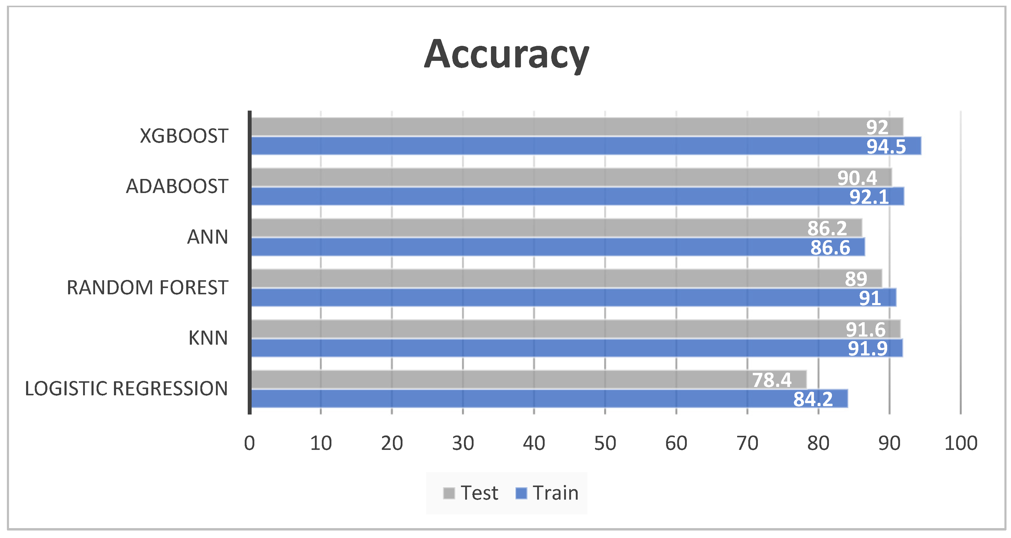
| XGBoost | 94.5 | 94.7 | 93.8 | 94.2 | 92 | 92 | 91 | 91.4 |
| AdaBoost | 92.1 | 88.9 | 91.2 | 90 | 90.4 | 90.1 | 89.5 | 89.8 |
| ANN | 86.6 | 84.9 | 83.2 | 84.1 | 86.2 | 88.2 | 83.1 | 85.7 |
| Random forest | 91 | 91.6 | 89.9 | 90.7 | 89 | 88.3 | 88.1 | 88.2 |
| KNN | 91.9 | 92.3 | 90.6 | 91.3 | 91.6 | 91.7 | 90.5 | 91 |
| Logistic Regression | 84.2 | 73.3 | 63.8 | 68.2 | 78.4 | 70 | 60.1 | 64.7 |
| Reference | Dataset Origin | ML Models Used | No of Parameters Considered | Accuracy | Feature Importance |
|---|---|---|---|---|---|
| [48] | Mexico | Five | 10 | 94.99% | No |
| [49] | Mexico | Various ML models | 21 | 93.50% | No |
| [51] | Mexico | Various ML models | - | 69% | No |
| [52] | Mexico | Various ML models | 22 | Sensitivity-75% | Gini Index |
| [53] | Mexico | Various ML models | 14 | Qualitative | No |
| Proposed | Mexico | Six | 10 | 94.50% | SHAP and LIME |
Publisher’s Note: MDPI stays neutral with regard to jurisdictional claims in published maps and institutional affiliations. |
© 2022 by the authors. Licensee MDPI, Basel, Switzerland. This article is an open access article distributed under the terms and conditions of the Creative Commons Attribution (CC BY) license (https://creativecommons.org/licenses/by/4.0/).
Share and Cite
Pradhan, A.; Prabhu, S.; Chadaga, K.; Sengupta, S.; Nath, G. Supervised Learning Models for the Preliminary Detection of COVID-19 in Patients Using Demographic and Epidemiological Parameters. Information 2022, 13, 330. https://doi.org/10.3390/info13070330
Pradhan A, Prabhu S, Chadaga K, Sengupta S, Nath G. Supervised Learning Models for the Preliminary Detection of COVID-19 in Patients Using Demographic and Epidemiological Parameters. Information. 2022; 13(7):330. https://doi.org/10.3390/info13070330
Chicago/Turabian StylePradhan, Aditya, Srikanth Prabhu, Krishnaraj Chadaga, Saptarshi Sengupta, and Gopal Nath. 2022. "Supervised Learning Models for the Preliminary Detection of COVID-19 in Patients Using Demographic and Epidemiological Parameters" Information 13, no. 7: 330. https://doi.org/10.3390/info13070330